I Introduction

The MHV vertex expansion, due to Cachazo et al (CSW) Cachazo:2004kj , is a diagrammatic method for calculating gauge theory scattering amplitudes. This method, inspired by Witten’s twistor string Witten:2003nn formulation of $\mathcal{N}=4$ super-Yang–Mills (SYM), often produces very simple expressions. While it is expected to be generally valid, to date it has been successfully used at tree and one-loop level Brandhuber:2004yw . This expansion can in fact be formally derived from the light-cone gauge fixed Yang-Mills action Gorsky:2005sf ; Mansfield:2005yd ; Ettle:2006bw and it can be shown to be equivalent to the Feynman diagram expansion of the twistor space Yang-Mills action Boels:2007qn .

In closely related developments, by studying the analytic properties of amplitudes as functions of complex external momenta, Britto et al (BCFW) found recursion relations which generate all tree-level amplitudes Britto:2004ap ; Britto:2005fq . The supersymmetric generalizations of these relations were solved explicitly Drummond:2008cr giving relatively compact expressions for all tree-level superamplitudes. By related analytic methods in which all external lines are taken to be complex, the MHV vertex expansion, Risager:2005vk ; Elvang:2008vz was directly reproduced, thus showing that the BCFW recursion relations and the MHV vertex expansion are equivalent at tree level.

The ${\cal N}=4$ SYM tree-level amplitudes constructed in Drummond:2008cr possess remarkable, hidden, conformal symmetries Drummond:2008cr ; Brandhuber:2008pf . Hints of these dual conformal symmetries were first seen in Drummond:2006rz , and extended to dual superconformal symmetry in Drummond:2008vq . For tree-level scattering amplitudes there is in fact an enhancement of superconformal symmetry to an infinite-dimensional algebra called the Yangian Drummond:2009fd .

The variables which make the dual conformal symmetry most apparent are the “momentum twistors” introduced by Hodges Hodges:2009hk . These momentum twistors, which are algebraically related to the null momenta of the amplitude and solve the overall momentum constraint, are the spinors of the dual conformal group. Perhaps the most elegant formulation of the Yangian invariants of ${\cal N}=4$ SYM is the Grassmannian. The original Grassmannian in standard twistor space was introduced in ArkaniHamed:2009dn where it was shown that a contour integral over the Grassmannian $G(k,n)$ produced the N^k-2MHV superamplitudes. An equivalent form in momentum twistor space was soon found Mason:2009qx which made the dual superconformal symmetry manifest. That the Grassmannian has the full Yangian symmetry was directly shown in Drummond:2010qh . For appropriate choices of the contour, the Grassmannian generates more than tree-level amplitudes, indeed it was argued Korchemsky:2010ut ; Drummond:2010uq that it generates all Yangian invariants.

Beyond tree-level, IR divergences in amplitudes can no longer be avoided and care must be taken in either regulating these divergences or in choosing to study objects which are well defined in spite of the bad IR behavior. A set of such objects are the integrands of the loop integrals. While in general such objects are ambiguous, as explained by Arkani-Hamed et al ArkaniHamed:2010kv (ABCCT), they can be canonically defined in the planar limit. ABCCT further introduced a recursive method (see also Boels:2010nw for related work), analogous to the BCFW recursion relations, for calculating the all-loop integrand starting from tree amplitudes. These recursion relations, in addition to providing an efficient method for calculating the integrands, make their Yangian invariance manifest.

As was shown by Bullimore et al (BMS) Bullimore:2010pj , the MHV vertex expansion can also be usefully recast in momentum twistor space, making the dual superconformal symmetry manifest. In this formulation the “propagators” are dual superconformal invariants while the vertices are simply unity. Using this formalism BMS gave an algorithm for calculating any tree-level amplitude and any loop integrand. As mentioned by BMS the expressions for the tree amplitudes are very similar to those found by solving the BCFW recursion relations and one might expect this to continue to be true for the loop integrand. In this work we confirm that expectation.

We start in Sec. (III), after a brief review of the momentum space recursion relations and MHV vertex expansion in Sec. (II), by showing that the tree amplitudes following from the momentum twistor MHV expansion satisfy the BCFW recursion relations. While this is in essence already known, we find that it is a very useful warm-up for the loop integrand calculation as many details are similar. In particular, while the MHV expansion naturally produces sums over rooted tree diagrams, we find it useful to recast it as sums over non-crossing partitions (which are well known to be equivalent e.g. Stanley ). Turning to the loop integrands in Sec. (IV) we explicitly study two examples - one-loop MHV and one-loop NMHV - and show that the MHV expansions satisfy the ABCCT recursion relations. We then introduce a rewriting of the sum over diagrams for the MHV expansion for all legs and all loops as a sum over a generalized class of non-crossing partitions, and show that it satisfies the ABCCT recursion relations. The use of non-crossing partitions enables us to write down the all-loop integrands in an explicit and concise way, and it makes the full classification of (graphs dual to) planar MHV diagrams clearer. As a side result we find a recursive relation for the number of elements in a certain class of non-crossing partitions, or equivalently, graphs dual to MHV diagrams. In App.(A), we further explain the one-to-one correspondence between non-crossing partitions and planar MHV diagrams. By rewriting the expansion in terms of dual graphs, the connections to the recently proposed dual supersymmetric Wilson loops Mason:2010yk ; CaronHuot:2010ek become more transparent.

This result can be viewed in several ways. Firstly, while the MHV vertex expansion is believed to be correct to all orders this has never been proved beyond one-loop, this work can be seen as providing evidence for the validity of the MHV expansion in showing that it is equivalent to the recursion relations following from analytic properties of the amplitudes. Secondly, it provides an explicit solution to the recursion relations of ABCCT analogous to that found at tree-level Drummond:2008cr , An important feature of the solution is that it is manifestly cyclic, thus it naturally unifies different forms of all-loop integrands from ABCCT relations with different shifts, and implies highly non-trivial relations between them.

II A brief review of recursion relations and MHV vertex expansion in momentum-twistor space

In this section, we shall give a brief review of the recursion relations and MHV vertex expansion in momentum-twistor space, for all-loop integrands of scattering amplitudes in planar $\mathcal{N}=4$ SYM. More details can be found in ArkaniHamed:2010kv ; Bullimore:2010pj .

II.1 Momentum twistors for planar $\mathcal{N}=4$ SYM

The $n$-particle superamplitude in planar $\mathcal{N}=4$ SYM, $\mathcal{A}(\lambda_{1},\tilde{\lambda}_{1},\tilde{\eta}_{1};\ldots;\lambda_{n},\tilde{\lambda}_{n},\tilde{\eta}_{n})$, depends on $n$ supermomenta, or equivalently, $n$ pairs of spinors $(\lambda^{\alpha}_{i},\tilde{\lambda}^{\dot{\alpha}}_{i})$, and $n$ fermionic variable $\tilde{\eta}^{I}_{i}$, for $i=1,\ldots,n$.

Due to the color-ordering, one can define $n$ region supermomenta $(x^{\alpha{\dot{\alpha}}}_{i},\theta^{\alpha I}_{i})$ by,

$$x_{i}-x_{i+1}=\lambda_{i}\tilde{\lambda}_{i},$$

$$\theta_{i}-\theta_{i+1}=\lambda_{i}\tilde{\eta}_{i},$$ (1)

where $(x_{n+1},\theta_{n+1})=(x_{1},\theta_{1})$, thus the supermomentum conservation $\sum_{i}\lambda_{i}\tilde{\lambda}_{i}=0,\sum_{i}\lambda_{i}\tilde{\eta}_{i}=0$, is automatically satisfied.

To make the dual superconformal symmetry of $\mathcal{N}=4$ SYM manifest, one introduce $n$ momentum supertwistors,

$$\mathcal{Z}^{A}_{i}=\left(\begin{array}[]{ll}&\lambda^{\alpha}_{i}\\ &\mu^{\dot{\alpha}}_{i}\\ &\eta^{I}_{i}\\ \end{array}\right)=\left(\begin{array}[]{ll}&\lambda^{\alpha}_{i}\\ &x^{\alpha\dot{\alpha}}_{i}\lambda^{\alpha}_{i}\\ &\theta^{\alpha I}_{i}\lambda^{\alpha}_{i}\end{array}\right),$$ (8)

which are defined projectively, for $i=1,\ldots,n$. The bosonic part of the momentum supertwistor is denoted as $Z_{i}=(\lambda_{i},\mu_{i})$, and henceforth we shall refer to $\mathcal{Z}_{i}$ simply as a momentum twistor.

The inverse map is given by,

$$x_{i}=\dfrac{\mu_{i}\lambda_{i-1}-\mu_{i-1}\lambda_{i}}{\langle i-1,i\rangle},$$

$$\theta_{i}=\dfrac{\eta_{i}\lambda_{i-1}-\eta_{i-1}\lambda_{i}}{\langle i-1,i\rangle},$$ (9)

where the 2-bracket is defined as $\langle a,b\rangle=\epsilon_{\alpha\dot{\alpha}}\lambda^{\alpha}_{a}\tilde{\lambda}^{\dot{\alpha}}_{b}$. Another set of useful relations express supermomenta in terms of momentum twistors,

$$\tilde{\lambda}_{i}=\dfrac{\mu_{i-1}\langle i,i+1\rangle+\mu_{i}\langle i+1,i-1\rangle+\mu_{i+1}\langle i-1,i\rangle}{\langle i-1,i\rangle\langle i,i+1\rangle}$$

$$\tilde{\eta}_{i}=\dfrac{\eta_{i-1}\langle i,i+1\rangle+\eta_{i}\langle i+1,i-1\rangle+\eta_{i+1}\langle i-1,i\rangle}{\langle i-1,i\rangle\langle i,i+1\rangle}.$$ (10)

The superamplitude $\mathcal{A}(1,\ldots,n)$ can be written in momentum-twistor space by pulling out the MHV tree amplitude $\mathcal{A}^{(0)}_{\rm{MHV}}(1,\ldots,n)$,

$$\mathcal{A}(1,\ldots,n)=\mathcal{A}^{(0)}_{\rm{MHV}}A(1,\ldots,n).$$ (11)

Henceforth we shall work with $A(1,\ldots,n)$, which is dual superconformal invariant. The geometric picture of amplitudes in momentum-twistor space is simple. The point $x_{i}$ is associated with the line $(i\,i+1)$ in momentum-twistor space, which is defined as the line passing through two (bosonic) points in the momentum-twistor space $Z_{i}$ and $Z_{i+1}$. Since the lines $(i-1\,i)$ and $(i\,i+1)$ intersect at $Z_{i}$, it is guaranteed that $x_{i}$ and $x_{i-1}$ are null separated, or equivalently, the mass-shell conditions $p_{i}^{2}=(x_{i}-x_{i+1})^{2}=0$ are automatically satisfied.

To see this explicitly, one can define the bosonic dual conformal invariants through the 4-bracket, $\langle a,b,c,d\rangle=\langle a\,b|c\,d\rangle=\epsilon_{ABCD}Z_{a}^{A}Z_{b}^{B}Z_{c}^{C}Z_{d}^{D}$, which vanishes if and only if the four points are coplanar, or equivalently, two lines, say, $(a\,b)$ and $(c\,d)$, intersect. For the case $(a,b,c,d)=(i-1,i,j-1,j)$, the 4-bracket is related to the Lorentz invariant,

$$(x_{i}-x_{j})^{2}=\frac{\langle i-1,i,j-1,j\rangle}{\langle i-1,i\rangle\langle j-1,j\rangle},$$ (12)

and we have seen that $(x_{i}-x_{j})^{2}=0$ if and only if the lines $(i-1\,i)$ and $(j-1\,j)$ intersect.

Furthermore, one can define the basic dual superconformal invariant using five momentum supertwistors,

$$[a,b,c,d,e]=\frac{\delta^{0|4}(\eta_{a}\langle b,c,d,e\rangle+cyclic)}{\langle a,b,c,d\rangle\langle b,c,d,e\rangle\langle c,d,e,a\rangle\langle d,e,a,b\rangle\langle e,a,b,c\rangle}.$$ (13)

As was shown in Mason:2009qx , for the special case $(a,b,c,d,e)=(n,i-1,i,j-1,j)$, it is given by the invariant $R_{n;i,j}$, which appears in the NMHV amplitude Drummond:2008cr ,

$$A^{(0)}_{\rm{NMHV}}=\sum_{1<i\prec j<n}R_{n;i,j},$$ (14)

where $i\prec j$ means $i<j-1$. However, $[a,b,c,d,e]$ is defined for five general momentum twistors, and we have seen that it has a simple pole when four of the five twistors become coplanar. Also it is obvious that the invariant is anti-symmetric for the five twistors, thus it vanishes whenever two of them are identified projectively. As we will see below, the invariant $[a,b,c,d,e]$ is the basic building block of planar amplitudes in momentum-twistor space.

II.2 BCFW recursion relations and loop generalizations in momentum-twistor space

The BCFW recursion relations for tree-level superamplitudes in $\mathcal{N}=4$ SYM have been reformulated in the momentum-twistor space ArkaniHamed:2010kv . The BCFW deformation has a simple form in momentum-twistor space, for which one needs to choose a special leg, say, $\mathcal{Z}_{1}$, to shift,

$$\mathcal{Z}_{1}\rightarrow\mathcal{Z}_{\hat{1}}=\mathcal{Z}_{1}+z\mathcal{Z}_{2}.$$ (15)

Then the color-ordered tree amplitude $M(1,\ldots,n)=A^{(0)}(1,\ldots,n)$ has poles $z_{j}$ where $\langle n,\hat{1},j-1,j\rangle=0$, for $j=4,\ldots,n-1$. The residue at the pole $z_{j}$ is given by the “inhomogeneous” term, $\int d^{0|4}\eta_{I_{j}}M(\hat{1}_{j},\ldots,j-1,I_{j})\frac{1}{P^{2}_{I_{j}}}M(I_{j},j,\ldots,n)$ where $\hat{1}_{j}$ and the internal leg $I_{j}$ is evaluated at the pole, and it simplifies significantly in momentum-twistor space ArkaniHamed:2010kv . In addition, there is a pole at infinity, $\mathcal{Z}_{\hat{1}}\rightarrow\mathcal{Z}_{2}$ projectively when $z\rightarrow\infty$, and its residue is non-vanishing. This corresponds to the “homogeneous” term with a $3$-point anti-MHV amplitude attached to $M_{n-1}$, and in momentum-twistor space, it is simply given by $M(2,\ldots,n)$. Adding all pieces together, the recursion relations for tree-level $n$-point N^kMHV amplitudes $M_{n,k}(1,\ldots,n)=A^{(0)}_{\rm{N}^{k}\rm{MHV}}(1,\ldots,n)$ can be written as,

$$M_{n,k}(1,\ldots,n) = M_{n-1,k}(2,\ldots,n)$$

$$+\sum_{j,k^{\prime}}~{}[j-1,j,n,1,2]~{}M_{j,k^{\prime}}(\hat{1}_{j},\ldots,j-1,I_{j})M_{n+2-j,k-1-k^{\prime}}(I_{j},j,\ldots,n)~{}.$$

The summation ranges are $j=4,\ldots,n-1,k^{\prime}=0,\ldots,k-1$ where terms with $k^{\prime}>j-4$ or $k-1-k^{\prime}>n-j-2$ obviously vanish, and the deformations are given by

$$\mathcal{Z}_{\hat{1}_{j}}=\langle 2,j-1,j,n\rangle\mathcal{Z}_{1}+\langle j-1,j,n,1\rangle\mathcal{Z}_{2}=(1\,2)\cap(j-1\,j\,n),$$

$$\mathcal{Z}_{I_{j}}=\langle j,n,1,2\rangle\mathcal{Z}_{j-1}+\langle n,1,2,j-1\rangle\mathcal{Z}_{j}=(j-1\,j)\cap(n\,1\,2).$$ (17)

Note in the second equalities we have adopted the geometric interpretation of the deformations ArkaniHamed:2010kv , where $(i\,j)\cap(k\,l\,m)$ denotes the intersect of line $(i\,j)$ with plane $(k\,l\,m)$.

Loop amplitudes in $\mathcal{N}=4$ SYM suffer from IR divergences. However, the integrands, which are not only IR-finite but simply rational functions, can be unambiguously defined in the planar sector and thus provide a well defined set of invariants which can be calculated. In order to do just that, a generalized set of BCFW-like recursion relations have been proposed for integrands for all-loop amplitudes in planar $\mathcal{N}=4$ SYM ArkaniHamed:2010kv . To specify the integrands of $l$-loop amplitudes, in addition to $n$ external momentum twistors, one also needs $l$ pairs of momentum twistors $(A_{m},B_{m})$, for $m=1,\ldots,l$, associated with $l$ loop momenta, upon which integrations are performed. For the $n$-point $l$-loop N^kMHV superamplitude, $A_{n,k,l}(1,\ldots,n)=A^{(l)}_{\rm{N}^{k}\rm{MHV}}(1,\ldots,n)$, the integrand $M_{n,k,l}(1,\ldots,n)$ can be defined by the generalized recursion relations ArkaniHamed:2010kv . The formula for $l$-loop integrand $M_{n,k,l}$ is similar to the tree-level one, plus a “source term” which comes from the poles $\langle n,\hat{1},A,B\rangle=0$ for $(A,B)=(A_{1},B_{1}),\ldots,(A_{l},B_{l})$,

$$M_{n,k,l}(1,\ldots,n;\{A,B\}_{l}) = M_{n-1,k,l}(2,\ldots,n;\{A,B\}_{l})+\frac{1}{l!}\sum_{\sigma_{l}}\sum_{j,k^{\prime}}~{}[n,1,2,j-1,j]~{}M^{L}~{}M^{R}$$ (18)

$$+\frac{1}{l}\sum^{l}_{l_{0}=1}\int_{\eta_{l_{0}}}\int_{GL(2)_{l_{0}}}[n,1,2,A_{l_{0}},B_{l_{0}}]M^{S},$$

with

$$M^{L}=M_{j,k^{\prime},l^{\prime}}(\hat{1}_{j},\ldots,j-1,I_{j};\{A,B\}_{L})$$

$$M^{R}=M_{n+2-j,k-1-k^{\prime},l-l^{\prime}}(I_{j},j,\ldots,n;\{A,B\}_{R})$$

$$M^{S}=M^{\prime}_{n+2,k+1,l-1}(\hat{1}_{A_{l_{0}}B_{l_{0}}},\ldots,n,A_{l_{0}},\hat{B}_{l_{0}};\{A,B\}_{\{l\}/l_{0}})$$ (19)

where in the second term on the r.h.s. of Eq.(18) we sum over all ways of distributing $\{A,B\}_{l}$ into $\{A,B\}_{L}$ with $l^{\prime}$ pairs of loop twistors and $\{A,B\}_{R}$ with $l-l^{\prime}$ pairs for $l^{\prime}=0,\ldots,l$, and introduce an $1/l!$ factor to compensate the overcounting; in the third term we sum over $l_{0}$ and introduce an $1/l$ factor. The various deformations are given by

$$\hat{1}_{j}=(1\,2)\cap(n\,j-1\,j),\, I_{j}=(j-1\,j)\cap(n\,1\,2),$$ (20)

$$\hat{1}_{AB}=(1\,2)\cap(n\,A\,B),\, \hat{B}=(A\,B)\cap(n\,1\,2),$$

with $(A,B)=(A_{l_{0}},B_{l_{0}})$ for $l_{0}=1,\ldots,l$.

The source term, as given by the last line of Eq. (18) is defined as the forward limit of integrands at $l-1$ loop order. Given the prefactor and $M_{n+2,k+1,l-1}$, the fermionic integration $\int_{\eta}=\int d^{0|4}\eta_{A}d^{0|4}\eta_{B}$ removes two of the total $k+2$ fermionic delta functions to produce a result in the N^kMHV sector. The “$GL(2)$” integration $\int_{GL(2)}$ is a contour integral over general $GL(2)$ transformations $g$, which bring an arbitrary $2$-vector $(A=\mathcal{Z}_{A},B=\mathcal{Z}_{B})$ to general $2$-vectors $(A^{\prime}=g_{11}A+g_{12}B,B^{\prime}=g_{21}A+g_{22}B)$, and the residue is given at the pole $A^{\prime}\propto B^{\prime}\propto\hat{B}$, or geometrically when both $A$ and $B$ lie on the plane $(n,1,2)$. As we shall explain in details shortly, the integrations in the source term imply that the integrand only depends on the lines $x_{(AB)_{1}},\ldots,x_{(AB)_{l}}$, or equivalently on the loop momenta, $p_{m}=x_{(AB)_{m}}-x_{(AB)_{m+1}}$, for $m=1,\ldots,l$. Thus the momentum-twistor space amplitudes are given by the usual loop integrations,

$$A_{n,k,l}(1,\ldots,n)=\prod^{l}_{m=1}\int d^{4}x_{(AB)_{m}}M_{n,k,l}(1,\ldots,n;\{x_{(AB)_{1}},\ldots,x_{(AB)_{l}}\}).$$ (21)

II.3 MHV vertex expansion in momentum-twistor space

Here we review the momentum-twistor space MHV vertex expansion for $\mathcal{N}=4$ SYM as formulated in Bullimore:2010pj and to where we point the reader for further details. The $n$-point N^kMHV tree-level superamplitude $M_{n,k}$ is given by the sum of all tree-level MHV diagrams with $k$ propagators and $k+1$ MHV vertices. Each diagram is given as a product of factors from vertices and propagators. Each vertex is given by unity, and for each propagator separating region momenta $x_{i},x_{j}$, one assigns a factor $[\ast,\widehat{i-1},i,\widehat{j-1},j]$, where $\ast$ is an arbitrary reference momentum twistor, and the possible deformation $\widehat{i-1}$ is defined as (and similarly for $\widehat{j-1}$),

$$\widehat{i-1}=\left\{\begin{array}[]{ll}i-1,&\textit{if $i-1$ is attached to the propagator,}\\ \hbox{\multirowsetup\mbox{$(i-1\,i)\cap(\ast\,k-1\,k)$},}&\textit{otherwise, where $(k-1k)$ is associated}\\ &\textit{~{}~{}with the preceding propagator},\end{array}\right.$$ (25)

where since region momenta are ordered increasingly, “preceding” means on the $i-1$ side. In Bullimore:2010pj , it has been shown that by choosing $\mathcal{Z}_{\ast}=(0,\iota^{\dot{\alpha}},0)$, the above rules reproduce the usual momentum-space MHV diagrams with reference spinor $\iota$.

Beyond tree level, in Bullimore:2010pj , the MHV vertex expansion in the planar sector is conjectured to calculate the loop integrands. The integrands defined by the recursion relations, $M_{n,k,l}$, depend on external twistors and loop momenta, but the integrands defined from the MHV vertex expansion, $M^{\prime}_{n,k,l}(1,\ldots,n;\{A_{1},B_{1},\ldots,A_{l},B_{l}\})$, are dual superconformal invariants, which generally depend on $n$ external twistors and $l$ pairs of loop twistors. By fully integrating over $2l$ loop momentum super-twistors, one obtains the loop amplitudes,

$$A_{n,k,l}(1,\ldots,n)=\prod^{l}_{m=1}\int d^{3|4}\mathcal{Z}_{A_{m}}d^{3|4}\mathcal{Z}_{B_{m}}M^{\prime}_{n,k,l}(1,\ldots,n;\{A_{1},B_{1},\ldots,A_{l},B_{l}\}).$$ (26)

Before reviewing the loop-level MHV vertex expansion we first explain the relation between $M_{n,k,l}$ and $M^{\prime}_{n,k,l}$. The integration measure of a pair of loop twistors can be split as

$$d^{3|4}\mathcal{Z}_{A}d^{3|4}\mathcal{Z}_{B}=\langle\lambda_{A}d\lambda_{A}\rangle\langle\lambda_{B}d\lambda_{B}\rangle\langle\lambda_{A}\lambda_{B}\rangle^{2}d^{4}x_{AB}d^{0|4}\eta_{A}d^{0|4}\eta_{B},$$ (27)

where, in addition to the fermionic integration measure, $d^{4}x_{AB}$ is the usual loop integral measure, interpreted as a measure on the choice of lines $x_{AB}$ through a pair of bosonic momentum twistors $Z_{A},Z_{B}$, and the measure of spinors is on the positions of $Z_{A},Z_{B}$ on the line $x_{AB}$. Now an equivalent way to integrate over positions on the line is to integrate over all $GL(2)$ transformations, thus we can write the integration over any pair of loop twistors $A,B$, as the loop momentum integration, the fermionic integration, and the $GL(2)$ integration,

$$\int d^{3|4}\mathcal{Z}_{A}d^{3|4}\mathcal{Z}_{B}M^{\prime}_{n,k,l}(A,B)=\int d^{4}x_{AB}\int d^{0|4}\eta_{A}d^{0|4}\eta_{B}\int\langle g_{1}dg_{1}\rangle\langle g_{2}dg_{2}\rangle\langle g_{1}g_{2}\rangle^{2}M^{\prime}_{n,k,l}(A^{\prime},B^{\prime})\,$$ (28)

where the two $2$-vectors $g_{1}=(g_{11},g_{12})$ and $g_{2}=(g_{21},g_{22})$ represent a $GL(2)$ transformation, $g$, that brings $(A,B)$ to $(A^{\prime},B^{\prime})=(A,B)g^{T}=(g_{11}A+g_{12}B,g_{21}A+g_{22}B)$.

Therefore, the relation between the two versions of integrands is,

$$M_{n,k,l}=\prod^{l}_{m=1}\int_{\eta_{m}}\int_{GL(2)_{m}}M^{\prime}_{n,k,l},$$ (29)

where the fermionic and $GL(2)$ integrations for $A_{m},B_{m}$, given by Eq. (28), have been denoted as $\int_{GL(2)_{m}}$ and $\int_{\eta_{m}}$, respectively. For tree-level amplitudes $M^{\prime}_{n,k,0}=M_{n,k,0}=M_{n,k}$. At loop level, the complete result from MHV diagrams in momentum-twistor space is supposed to be independent of the positions of $Z_{A},Z_{B}$ on the line $x_{AB}$, which makes any $GL(2)$ integration trivial and yield a constant Bullimore:2010pj . However, it is non-trivial to see the independence of the result on the $GL(2)$ part of the integration term by term in the momentum twistor formulation.

Now we briefly review the MHV vertex expansion for the loop integrands $M^{\prime}_{n,k,l}$ in momentum-twistor space Bullimore:2010pj . The integrand $M^{\prime}_{n,k,l}$ is given by the sum of all $l$-loop planar MHV diagrams with $2l$ loop twistors and cyclically ordered $n$ external twistors. Each MHV diagram is given by the product of factors coming from $k+2l$ propagators and some vertices. Each vertex is again given by unity, and each propagator is given by $[\ast,\,,\,,\,,\,]$ which depends on a reference twistor and four other momentum twistors specified by the following rules.

For a propagator separating regions of external momenta, $x_{i}$ and $x_{j}$, the four twistors needed are $\widehat{i-1},i,\widehat{j-1},j$, where the deformation is defined as for tree amplitudes, except that the preceding region momentum $(k-1\,k)$ can be a loop region momentum labeled by $A_{m},B_{m}$. For a propagator which separates $x_{i}$ from loop region $x_{(AB)_{m}}$, we need $\widehat{i-1},i,A_{m},\widehat{B_{m}},$ with $\widehat{B_{m}}=(A_{m}\,B_{m})\cap(\ast\,k-1\,k)$ where $(k-1\,k)$ is the preceding region momentum, which can be either an external or a loop region. For a propagator separating $x_{(AB)_{m}}$ and $x_{(AB)_{m^{\prime}}}$, we need $A_{m},\widehat{B_{m}},A_{m^{\prime}},\widehat{B_{m^{\prime}}}$ with similarly deformed loop twistors.

III Tree amplitudes

As a warm-up for loop-level integrands, in this section we will prove that the MHV vertex expansion for tree amplitudes provides an explicit solution to the BCFW recursion relations. After working out some examples, we will rewrite the expansion for general tree amplitudes and prove its validity.

III.1 Examples

MHV  The MHV amplitude becomes trivial in momentum-twistor space, $M_{n,0}=1$, which automatically satisfies Eq.(II.2) since there is no inhomogeneous terms.

NMHV  For $k=1$, Fig. (1),

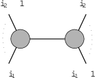
Figure 1: Vertex diagram for NMHV amplitude

we have a summation over a pair of region momenta which label the propagator,

$$M_{n,1}=\sum_{i_{1}\prec i_{2}\prec i_{1}+n}[\ast,i_{1}-1,i_{1},i_{2}-1,i_{2}],$$ (30)

where no deformation is needed, and instead of the standard summation range $i_{1}\leq i_{2}\leq i_{1}+n$ we have used, for example, $i_{1}\prec i_{2}$ to denote $i_{1}<i_{2}-1$ module $n$. Due to the total antisymmetry of the basic invariant, terms with $i_{1}-i_{2}=0,\pm 1$ simply vanish. To compare with Eq. (II.2), it is convenient to choose $\ast=n$, then the summation range becomes $2\leq i_{1}\prec i_{2}\leq n-1$ and we have,

$$M_{n,1}=\sum_{2\leq i_{1}\prec i_{2}\leq n-1}[n,i_{1}-1,i_{1},i_{2}-1,i_{2}].$$ (31)

This immediately follows from Eq. (II.2) given that both subamplitudes must be MHV amplitudes, that is to say, simply unity. This result is of course nothing but the well known result Eq. (14). Note that the MHV vertex expansion is independent of the choices of $\ast$, thus Eq. (30) provides a cyclically invariant explicit solution to the BCFW recursion relations.

N²MHV  For $k=2$, Fig.(2),

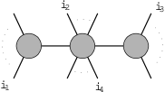
Figure 2: Vertex diagram for NMHV amplitude

the summation is over two pairs of region momenta, $i_{1}\prec i_{2}\leq i_{3}\prec i_{4}\leq i_{1}+n$,

$$M_{n,2}=\sum_{i_{1},i_{2},i_{3},i_{4}}[\ast,\widehat{i_{1}-1},i_{1},i_{2}-1,i_{2}][\ast,\widehat{i_{3}-1},i_{3},i_{4}-1,i_{4}],$$ (32)

where the summation range has been indicated before, and, from the deformation rule, we know that when $i_{1}=i_{4}$ module $n$, a deformation is needed, $\widehat{i_{1}-1}=(i_{1}-1\,i_{1})\cap(\ast\,i_{3}-1\,i_{3})$, and when $i_{3}=i_{2}$, $\widehat{i_{3}-1}=(i_{3}-1\,i_{3})\cap(\ast\,i_{1}-1\,i_{1})$ (these two boundary cases can not happen simultaneously since the middle vertex must have at least three legs).

Again one chooses $\ast=n$, then for $M_{n,2}(1,\ldots,n)$ the summation range can be split into two cases, $2\leq i_{1}\prec i_{2}\leq i_{3}\prec i_{4}\leq n-1$ and $2\leq i_{2}\leq i_{3}\prec i_{4}\leq i_{1}\leq n-1$, and similarly for $M_{n-1,2}(2,\ldots,n)$ with both lowest limits being $3$. This corresponds to summing over the two inequivalent “rootings”of the “1” leg, i.e. on the first and middle vertex. Then the difference in recursion relations is given by terms in the first range with $i_{1}=2$ and those in the second range with $i_{2}=2$

$$M_{n,2}(1,\ldots,n)-M_{n-1,2}(2,\ldots,n) = \sum_{4\leq i_{2}\leq i_{3}\prec i_{4}\leq n-1}[n,1,2,i_{2}-1,i_{2}][n,\widehat{i_{3}-1},i_{3},i_{4}-1,i_{4}]$$ (33)

$$\kern-30.0pt+\sum_{2\leq i_{3}\prec i_{4}\leq i_{1}\leq n-1}[n,\widehat{i_{1}-1},i_{1},1,2][n,\widehat{i_{3}-1},i_{3},i_{4}-1,i_{4}].$$

Now from Eq. (30), with the choice $\ast=n$, we have for the NMHV subamplitude

$$M_{n+2-i_{2},1}(I_{i_{2}},i_{2},...,n)=\sum_{i_{2}\leq i_{3}\prec i_{4}\leq n-1}[n,\widehat{i_{3}-1},i_{3},i_{4}-1,i_{4}]$$ (34)

because the deformation needed when $i_{3}=i_{2}$ is exactly $\widehat{i_{2}-1}=I_{i_{2}}$. Thus the first sum in Eq. (33) simply gives $\sum_{4\leq i_{2}\leq i_{3}\prec i_{4}\leq n-1}[n,1,2,i_{2}-1,i_{2}]M_{i_{2},0}(1_{i_{2}},\ldots,i_{2}-1,I_{i_{2}})M_{n+2-i_{2},1}(I_{i_{2}},i_{2},\ldots,n)$.

For the second sum, we note that due to orientation reversal symmetry Bullimore:2010pj we have the identity,

$$[n,\widehat{i_{1}-1},i_{1},1,2][n,\widehat{i_{3}-1},i_{3},i_{4}-1,i_{4}]=[n,i_{1}-1,i_{1},1,2][n,\widehat{i_{3}-1},i_{3},i_{4}-1,\widehat{i_{4}}]$$ (35)

where $\widehat{i_{4}}=(i_{1}-1\,i_{1})\cap(n\,1\,2)$ if $i_{4}=i_{1}$ and it is simply $i_{4}$ otherwise. Thus the second sum is equal to $\sum_{2\leq i_{3}\prec i_{4}\leq i_{1}\leq n-1}[n,1,2,i_{1}-1,i_{1}][n,\widehat{i_{3}-1},i_{3},i_{4}-1,\widehat{i_{4}}]=\sum_{2\leq i_{3}\prec i_{4}\leq i_{1}\leq n-1}[n,1,2,i_{1}-1,i_{1}]M_{i_{1},1}(1_{i_{1}},\ldots,i_{1}-1,I_{i_{1}})M_{n+2-i_{1},0}(I_{i_{1}},i_{1},...,n)$, where we have used $\widehat{i_{3}-1}=1_{i_{1}}$ if $i_{3}=2$ and $\widehat{i_{4}}=I_{i_{1}}$ when $i_{4}=i_{1}$. Therefore, we see that Eq. (32)also satisfies the recursion relations.

III.2 General tree amplitudes

Generally for N^kMHV tree amplitudes, in addition to summing over the distributions of $n$ legs into $2k$ ordered subsets labeled by region momenta, $i_{1}\leq i_{2}\leq\ldots\leq i_{2k}\leq i_{1}+n$, one also needs to sum over all types of MHV diagrams. To be concrete, one needs to pick a root, then there are $C_{k}=\frac{(2k)!}{k!(k+1)!}$ (the Catalan number) types of diagrams to be summed over, namely, all rooted trees with $k$ edges. It is well known that they are in one-to-one correspondence with all non-crossing partitions of the sequence $i_{1},i_{2},\ldots,i_{2k-1},i_{2k}$ into $k$ pairs, where each pair simply labels two region separated by an edge of the rooted tree. Here “non-crossing” means that for the sequence $a,b,c,d$, one can have $\{(a,b),(c,d)\},\{(a,d),(c,b)\}$ as valid partitions but not $\{(a,c),(b,d)\}$.

Each partition can be represented by a forest graph in which each region is represented by a vertex and each pair by an edge. The non-crossing partitions consists of the set of forests for which edges only intersect at vertices. We denote the set of such partitions, or equivalently rooted trees, as $J_{k}$. For example, $J_{1}=\{\{i_{1},i_{2}\}\},J_{2}=\{\{i_{1},i_{2};i_{3},i_{4}\},\{i_{1},i_{4};i_{2},i_{3}\}\}$, and $J_{3}=\{\{i_{1},i_{2};i_{3},i_{4};i_{5},i_{6}\},\{i_{1},i_{2};i_{3},i_{6};i_{4},i_{5}\},\{i_{1},i_{4};i_{2},i_{3};i_{5},i_{6}\},\{i_{1},i_{6};i_{2},i_{3};i_{4},i_{5}\},\{i_{1},i_{6};i_{2},i_{5};i_{3},i_{4}\}\}$. As an example we show graphs corresponding to the elements of $J_{3}$ in Fig. (3).

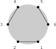
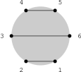
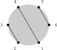
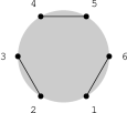
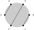
Figure 3: Elements of $J_{3}$

The relationship to geometric dual diagrams should be apparent and we will make this more concrete later when we consider diagrams with loops.

Given that the sequence $i_{1},\ldots,i_{2k}$ labels all $2k$ ordered region momenta, each pair in a non-crossing partition corresponds to a propagator in a MHV diagram. Thus the tree amplitudes $M_{n,k}$ given by MHV vertex expansion can be written in an explicit form,

$$M_{n,k}=\sum_{1\leq i_{1}\leq\ldots\leq i_{2k}\leq n}\sum_{j^{\alpha}\in J_{k}}\prod^{k}_{m=1}[\ast,\widehat{j^{\alpha}_{2m-1}-1},j^{\alpha}_{2m-1},\widehat{j^{\alpha}_{2m}-1},j^{\alpha}_{2m}],$$ (36)

where the first summation is over all distributions of legs, and the second over all non-crossing partitions $j^{\alpha}$, where $j^{\alpha}_{2m-1}$ and $j^{\alpha}_{2m}$ correspond to a region pair $(m=1,\ldots,k)$ in the partition $j^{\alpha}$. In addition, given a pair $j_{m+1}^{\alpha}=i_{l^{\prime\prime}}$, $j^{\alpha}_{m}=i_{l}$, we have the definition: $\widehat{j^{\alpha}_{m}-1}=(i_{l}-1\,i_{l})\cap(\ast\,i_{l^{\prime}}-1\,i_{l^{\prime}})$ if $i_{l}=i_{l-1}$, with $(i_{l-1},i_{l^{\prime}})$ the pair in the partition which precedes $(i_{l},i_{l^{\prime\prime}})$, and $\widehat{j^{\alpha}_{m}-1}=i_{l}-1$ otherwise.

As a final tree-level example, we write down the N³MHV amplitude corresponding to Fig. (3), denoting $\prod^{k}_{m=1}[\ast,\widehat{j_{2m-1}-1},j_{2m-1},\widehat{j_{2m}-1},j_{2m}]$ by $[\widehat{j_{1}},\widehat{j_{2}};\ldots;\widehat{j_{2k-1}},\widehat{j_{2k}}]$, we have

$$M_{n,3} = \sum_{i_{1}\leq\ldots\leq i_{6}}[i_{1},i_{2};\widehat{i_{3}},i_{4};\widehat{i_{5}},i_{6}]+[i_{1},i_{2};\widehat{i_{3}},\widehat{i_{6}};\widehat{i_{4}},i_{5}]+[i_{1},\widehat{i_{4}};\widehat{i_{2}},i_{3};\widehat{i_{5}},i_{6}]+[i_{1},\widehat{i_{6}};\widehat{i_{2}},i_{3};\widehat{i_{4}},i_{5}]$$ (37)

$$\kern 25.0pt+~{}[i_{1},\widehat{i_{6}};\widehat{i_{2}},\widehat{i_{5}};\widehat{i_{3}},i_{4}].$$

Now it is straightforward to prove that Eq. (36) provides an explicit solution to BCFW recursion relations, Eq. (II.2). As always, it is convenient to choose $\ast=n$, then taking the difference of $M_{n,k}(1,\ldots,n)$ and $M_{n-1,k}(2,\ldots,n)$ we are left with all terms such that $i_{1}=2$. The amplitude involves all non-crossing pairings of $i_{1}$ with all other regions, $i_{2},i_{4},\ldots,i_{2k}$. Given a choice of pairing, say, $(i_{1},i_{4})$, subset of partitions in $J_{k}$ with this choice consists of all products of non-crossing partitions of $i_{2},i_{3}$ i.e. $J_{1}(i_{2},i_{3})$ and $i-5,\dots,i_{2k}$, i.e. $J_{k-2}(i_{5},\dots,i_{2k})$. More generally, $J_{k}$ can be split into (with a slight abuse of notation),

$$J_{k} = \{i_{1},i_{2};J_{k-1}(i_{3},\ldots,i_{2k})\}\cup\{i_{1},i_{4};J_{2}(i_{2},i_{3});J_{k-2}(i_{5},\ldots,i_{2k})\}\cup\ldots$$ (38)

$$~{}~{}~{}\dots\cup\{i_{1},i_{2k};J_{k-1}(i_{2},\ldots,i_{2k-1})\}.$$

This is graphically shown in Fig.(4).

$\Rightarrow$  

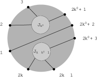
Figure 4: Factorization of non-crossing partition about the pair $(i_{1},i_{2m^{\prime\prime}})$.

In this way, the summation over $j^{\alpha}$ splits into $k$ double summations, labeled by $k^{\prime}=0,\ldots,k-1$. Each one consists of a summation over $j^{\prime\alpha}\in J_{k^{\prime}}(i_{2},\ldots,i_{2k^{\prime}+1})$, a summation over $j^{\prime\prime\alpha}\in J_{k-k^{\prime}-1}(i_{2k^{\prime}+3},\ldots,i_{2k})$, and there is a prefactor $[n,1,2,\widehat{i_{2k^{\prime}+2}-1},i_{2k^{\prime}+2}]$. The summation over distributions of legs can be written as a summation over $i_{2k^{\prime}+2}$, a summation over $1<i_{2}\leq\ldots\leq i_{2k^{\prime}+1}$, as well as a summation over $i_{2k^{\prime}+3}\leq\ldots\leq i_{2k}<n$. The remaining factors also split into the product of two corresponding pieces, $\prod^{k^{\prime}}_{m=1}[n,\widehat{j^{\prime\alpha}_{2m-1}-1},j^{\prime\alpha}_{2m-1},\widehat{j^{\prime\alpha}_{2m}-1},j^{\prime\alpha}_{2m}]$ and $\prod^{k-1-k^{\prime}}_{m=1}[n,\widehat{j^{\prime\alpha}_{2m-1}-1},j^{\prime\prime\alpha}_{2m-1},\widehat{j^{\prime\prime\alpha}_{2m}-1},j^{\prime\prime\alpha}_{2m}]$.

Therefore, the difference can be written as a sum of $k$ terms, each being a product of two summations. From Eq. (36), the second sum is,

$$\sum_{i_{2k^{\prime}+2}\leq i_{2k^{\prime}+3}\leq\ldots\leq i_{2k}<n}\sum_{j^{\prime\prime\alpha}\in J_{k-k^{\prime}-1}}\prod^{k-1-k^{\prime}}_{m=1}[n,\widehat{j^{\prime\prime\alpha}_{2m-1}-1},j^{\prime\prime\alpha}_{2m-1},\widehat{j^{\prime\prime\alpha}_{2m}-1},j^{\prime\prime\alpha}_{2m}]$$

$$\kern 160.0pt=M_{n+2-i_{2k^{\prime}+2},k-1-k^{\prime}}(\widehat{i_{2k^{\prime}+2}-1},i_{2k^{\prime}+2},\ldots,n),$$ (39)

where one always needs the deformation $\widehat{i_{2k^{\prime}+2}-1}=(i_{2k^{\prime}+2}-1\,i_{2k^{\prime}+2})\cap(n,1,2)$, which is exactly $I_{i_{2k^{\prime}+2}}$ in Eq. (20). On the other hand, due to the reversal symmetry, one can shift the deformation on $i_{2k^{\prime}+2}-1$ to $i_{2k^{\prime}+1}$, which is $\widehat{i_{2k^{\prime}+1}}=(i_{2k^{\prime}+2}-1\,i_{2k^{\prime}+2})\cap(n,1,2)=I_{i_{2k^{\prime}+2}}$, thus the first summation is,

$$\sum_{1<i_{2}\leq\ldots\leq i_{2k^{\prime}+1}\leq i_{2k^{\prime}+2}}\sum_{j^{\prime\alpha}\in J_{k^{\prime}}}\prod^{k^{\prime}}_{m=1}[n,\widehat{j^{\prime\alpha}_{2m-1}-1},j^{\prime\alpha}_{2m-1},\widehat{j^{\prime\alpha}_{2m}-1},j^{\prime\alpha}_{2m}]$$

$$\kern 160.0pt=M_{i_{2k^{\prime}+2},k^{\prime}}(\widehat{1},\ldots,i_{2k^{\prime}+2}-1,I_{i_{2k^{\prime}+2}}),$$ (40)

where $\widehat{1}=(1\,2)\cap(n\,i_{2k^{\prime}+2}-1\,i_{2k^{\prime}+2})$ is $\hat{1}_{i_{2k^{\prime}+2}}$ in Eq. (20). Therefore, we obtain,

$$M_{n,k}-M_{n-1,k}=\sum_{k^{\prime}=0,\ldots,k-1}\sum_{i_{2k^{\prime}+2}}[n,1,2,i_{2k^{\prime}+2}-1,i_{2k^{\prime}+2}]$$

$$\times M_{i_{2k^{\prime}+2},k^{\prime}}(\hat{1}_{i_{2k^{\prime}+2}},\ldots,i_{2k^{\prime}+2}-1,I_{i_{2k^{\prime}+2}})M_{n+2-i_{2k^{\prime}+2},k-1-k^{\prime}}(I_{i_{2k^{\prime}+2}},i_{2k^{\prime}+2},\ldots,n),$$ (41)

which is nothing but the BCFW recursion relations, Eq. (II.2).

Since the formula (36) is a rewriting of the momentum-space MHV vertex expansion, it must be independent of the reference twistor $\ast$. In fact, it is straightforward to check that by choosing $\ast$ to be other external twistors, the formula reproduces other forms of tree amplitudes, from BCFW recursion relations with other shifts. As discussed in Hodges:2009hk ; ArkaniHamed:2009dn , it is highly non-trivial to prove the equivalence of these different forms, which guarantees important properties, such as cyclic invariance and absence of spurious poles, of the tree amplitudes. It is significant that the formula obtained here relates different BCFW forms of the tree amplitude, and it is manifestly cyclically invariant.

IV All-loop Integrands

Now we move to integrands of all-loop amplitudes in the planar sector. The MHV vertex expansion becomes more involved at higher loops, so we will first examine carefully the one-loop MHV and NMHV integrands as solutions to the generalized recursion relations. Then we propose and prove a general formula for the MHV vertex expansion in terms of non-crossing partitions, as a straightforward generalization of the tree-level case.

IV.1 Examples of Loop Integrands

IV.1.1 One-loop MHV integrand

The MHV one-loop integrand, $M^{\prime}_{n,0,1}$, which only receives contribution from the “bubble” topology, is given by, Fig.(5),

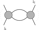
Figure 5: Vertex diagram for one-loop MHV amplitude

$$M^{\prime}_{n,0,1}=\sum_{i_{1}<i_{2}}[\ast,i_{1}-1,i_{1},A,B^{\prime}][\ast,i_{2}-1,i_{2},A,B^{\prime\prime}],$$ (42)

where $B^{\prime}=(A\,B)\cap(\ast\,i_{2}-1\,i_{2})$ and $B^{\prime\prime}=(A\,B)\cap(\ast\,i_{1}-1\,i_{1})$. We shall prove that Eq. (42), after doing fermionic and $GL(2)$ integrations, provides an explicit solution to Eq. (18). Each term of $M^{\prime}_{n,0,1}$ only depends on the line $(A,B)$ and we note that $(A\,B)=(A\,B^{\prime})$. Since $B^{\prime\prime}=(A\,B^{\prime})\cap(\ast\,i_{1}-1\,i_{1})$, and the fermionic and $GL(2)$ integration measure in $M_{n,0,1}$ are invariant under the shift $B\rightarrow B^{\prime}$, we have that (using the relation between integrands $M$ and $M^{\prime}$)

$$M_{n,0,1}=\sum_{i_{1}<i_{2}}\int_{\eta_{A{\tilde{B}}^{\prime}}}\int_{GL(2)_{A{\tilde{B}}^{\prime}}}[\ast,i_{1}-1,i_{1},A,{\tilde{B}}^{\prime}][\ast,i_{2}-1,i_{2},A,B^{\prime\prime}]~{}.$$ (43)

Here it is important to clarify the integration contour. The $GL(2)$ integration relating $M^{\prime}_{n,0,1}$ to $M_{n,0,1}$ is trivial. The $GL(2)_{A{\tilde{B}}^{\prime}}$ integration above should be understood as a contour integration forcing the dummy variable ${\tilde{B}}^{\prime}$ to lie in the plane defined by $(\ast\,i_{2}-1\,i_{2})$ i.e. at the point $B^{\prime}$. Now since after $GL(2)$ integration the result only depends on $x_{AB}$ which is also $x_{A{\tilde{B}}^{\prime}}$, we can shift it back,

$$M_{n,0,1}=\sum_{i_{1}<i_{2}}\int_{\eta}\int_{GL(2)}[\ast,i_{1}-1,i_{1},A,B][\ast,i_{2}-1,i_{2},A,B^{\prime\prime}].$$ (44)

Note that this is actually just a change of dummy variable because after integration $M_{n,0,1}$ only depends on $B$ through $x_{AB}$, which satisfies $x_{AB}=x_{AB^{\prime}}$.

If we choose $\ast=n$, then the difference between $M_{n,0,1}$ and $M_{n-1,0,1}$ is given by terms with $i_{1}=2$,

$$M_{n,0,1}-M_{n-1,0,1}=\int_{\eta}\int_{GL(2)}[n,1,2,A,B]\sum_{2<i_{2}<n}[n,i_{2}-1,i_{2},A,\hat{B}],$$ (45)

where we have used $B^{\prime\prime}=\hat{B}$ for $i_{1}=2$ and $\ast=n$. The only contribution in Eq. (18) for this case is the source term with $M_{n+2,1,0}(1_{AB},\ldots,n,A,\hat{B})$. As we will show shortly, in the NMHV tree amplitudes Eq. (30) with $\ast=n$, only terms which have at least one factor with both $A$ and $\hat{B}$ as arguments survive the fermionic integration. We conclude that the one-loop MHV integrand from the MHV vertex expansion satisfies the recursion relations.

We can in fact go further in this case as it is straightforward to explicitly perform the fermionic and $GL(2)$ integrations,

$$M_{n,0,1} = \sum_{1<i_{1}<i_{2}<n}\Big{[}\langle A\,B|(n\,i_{1}-1\,i_{1})\cap(n\,i_{2}-1\,i_{2})\rangle^{2}$$ (46)

$$\kern-60.0pt\times\frac{1}{\langle A,B,i_{1}-1,i_{1}\rangle\langle A,B,i_{1}-1,n\rangle\langle A,B,i_{1},n\rangle\langle A,B,i_{2}-1,i_{2}\rangle\langle A,B,i_{2}-1,n\rangle\langle A,B,i_{2},n\rangle}\Big{]},$$

where in the numerator $\langle AB|(n\,i_{1}-1\,i_{1})\cap(n\,i_{2}-1\,i_{2})\rangle=\langle A,n,i_{1}-1,i_{1}\rangle\langle B,n,i_{2}-1,i_{2}\rangle-\langle B,n,i_{1}-1,i_{1}\rangle\langle A,n,i_{2}-1,i_{2}\rangle$, with $(n\,i_{1}-1\,i_{1})\cap(n\,i_{2}-1\,i_{2})$ the intersecting line of the two planes, and, as promised, the $GL(2)$ integration renders each term only a function of line $x_{AB}$.

IV.1.2 A lemma for the source term

Here we prove a lemma for the source term: in the MHV vertex expansion of the integrand $M_{n+2,k+1,l-1}(\hat{1}_{AB},\ldots,n,A,\hat{B})$, only those terms, which have at least one factor with both loop twistors and no factor with a single loop twistor, survive the fermionic integration. This is crucial for relating MHV vertex expansion and recursion relations, since no other terms should appear in the MHV vertex expansion.

First, any factor with a single loop twistor, $A$ or $\hat{B}$, vanishes by itself. For convenience, we choose $\ast=n$ for the MHV vertex expansion of $M_{n+2,k+1,l-1}(\hat{1}_{AB},\ldots,n,A,\hat{B})$, then invariants with only $A$ vanish, $[n,x,y,n,A]=0$ for any $x,y$, and thus we focus on the factors with only $\hat{B}$, i.e. $[n,x,y,\hat{B},\hat{1}_{AB}]$.

Since $\hat{B}=(A\,B)\cap(n\,1\,2)$ and $\hat{1}_{AB}=(1\,2)\cap(n\,A\,B)$, $n,\hat{B}$ and $\hat{1}_{AB}$ must lie on the same line in the momentum-twistor space, and it is straightforward to write down the linear dependence,

$$\langle x,y,\hat{B},\hat{1}_{AB}\rangle\mathcal{Z}_{n}+\langle\hat{1}_{AB},n,x,y\rangle\mathcal{Z}_{\hat{B}}+\langle n,x,y,\hat{B}\rangle\mathcal{Z}_{\hat{1}_{AB}}=0,$$ (47)

for any $x,y$. In the fermionic delta function of $[n,x,y,\hat{B},\hat{1}_{AB}]$, the sum of the three terms with $\eta_{n},\eta_{\hat{B}}$ and $\eta_{\hat{1}_{AB}}$ vanishes since it is the fermionic part of the above expression, then we have,

$$[n,x,y,\hat{B},\hat{1}_{AB}]=\frac{\delta^{0|4}(\langle y,\hat{B},\hat{1}_{AB},n\rangle\eta_{x}+\langle\hat{B},\hat{1}_{AB},n,x\rangle\eta_{y})}{\langle\hat{1}_{AB},n,x,y\rangle\langle n,x,y,\hat{B}\rangle\langle x,y,\hat{B},\hat{1}_{AB}\rangle\langle y,\hat{B},\hat{1}_{AB},n\rangle\langle\hat{B},\hat{1}_{AB},n,x\rangle},$$ (48)

where, due to the linear dependence of $n,~{}\hat{B}$ and $\hat{1}_{AB}$, the numerator has four zeros from e.g. $\langle y,\hat{B},\hat{1}_{AB},n\rangle^{4}$ or $\langle\hat{B},\hat{1}_{AB},n,x\rangle^{4}$, and the denominator has two zeros from the last two factors, so it vanishes identically.

In addition, for any term to survive the fermionic integration over $\eta_{A},\eta_{B}$, one needs four $\eta_{A}$ and four $\eta_{B}$, which means the term must have at least two factors containing (possibly deformed) loop twistors. Since there is a prefactor $[n,1,2,A,B]$, this excludes any term in $M_{n+2,k+1,l-1}$ which has no factor with any loop twistors. Thus we have seen, only terms which have factor(s) with both $A$ and $\hat{B}$ and no factor with one of them, $A$ or $\hat{B}$, survive the fermionic integration.

IV.1.3 One-loop NMHV integrand

The next simplest case is the one-loop NMHV integrand, $M^{\prime}_{n,1,1}$. The MHV vertex expansion has contributions from both “triangle” and “bubble $+$ leg” topologies see Fig.(6), and the result is,

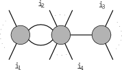
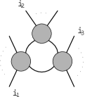
Figure 6: Bubble $+$ leg and triangle diagrams for one-loop NMHV amplitude

$$M^{\prime}_{n,1,1}=\sum_{i_{1}<i_{2}<i_{3}}[\ast,i_{1}-1,i_{1},A,B^{\prime}][\ast,i_{2}-1,i_{2},A,B^{\prime\prime}][\ast,i_{3}-1,i_{3},A,B^{\prime\prime\prime}]$$

$$+\sum_{i_{1}<i_{2}\leq i_{3}\prec i_{4}}[\ast,\widehat{i_{1}-1},i_{1},A,B^{*}][\ast,i_{2}-1,i_{2},A,B^{**}][\ast,\widehat{i_{3}-1},i_{3},i_{4}-1,i_{4}],$$ (49)

where in the first sum, $B^{\prime}=(A\,B)\cap(\ast\,i_{3}-1\,i_{3}),B^{\prime\prime}=(A\,B)\cap(\ast\,i_{1}-1\,i_{1})$, and $B^{\prime\prime\prime}=(A\,B)\cap(\ast\,i_{2}-1\,i_{2})$; in the second sum, deformations are needed, $\widehat{i_{1}-1}=(i_{1}-1\,i_{1})\cap(\ast\,i_{4}-1\,i_{4})$ when $i_{1}=i_{4}$ module $n$, $\widehat{i_{3}-1}=(i_{3}-1\,i_{3})\cap(\ast\,A\,B^{\prime\prime})$ when $i_{3}=i_{2}$, and we also have $B^{*}=(A\,B)\cap(\ast\,i_{2}-1\,i_{2}),B^{**}=(A\,B)\cap(\ast\,\widehat{i_{1}-1}\,i_{1})$.

Now we prove that Eq. (IV.1.3) also satisfies the recursion relations. Choosing $\ast=n$, and noting that in each term of the summation we can use the same trick as in the MHV case to replace $B^{\prime},{B^{\ast}}$ or ${B^{\ast}}$ by $B$ without changing anything else, then the difference of $M_{n,1,1}$ and $M_{n-1,1,1}$ is given by $i_{1}=2$ terms in the first sum, and terms with $i_{1}=2$ or $i_{2}=2$ or $i_{3}=2$ or $i_{4}=2$ in the second sum,

$$M_{n,1,1}-M_{n-1,1,1}=\int_{\eta}\int_{GL(2)}\{\sum_{2<i_{2}<i_{3}<n}[n,1,2,A,B][n,i_{2}-1,i_{2},A,B^{\prime\prime}][n,i_{3}-1,i_{3},A,\widehat{B^{\prime\prime}}]$$

$$+\sum_{2<i_{2}\leq i_{3}\prec i_{4}<n}[n,1,2,A,B][n,i_{2}-1,i_{2},A,B^{**}][n,\widehat{i_{3}-1},i_{3},i_{4}-1,i_{4}]$$

$$+\sum_{2\leq i_{3}\prec i_{4}\leq i_{1}<n}[n,\widehat{i_{1}-1},i_{1},A,B^{*}][n,1,2,A,B][n,\widehat{i_{3}-1},i_{3},i_{4}-1,i_{4}]$$

$$+\sum_{3<i_{4}\leq i_{1}<i_{2}<n}[n,\widehat{i_{1}-1},i_{1},A,B^{*}][n,i_{2}-1,i_{2},A,B^{**}][n,1,2,i_{4}-1,i_{4}]$$

$$+\sum_{2\leq i_{1}<i_{2}\leq i_{3}<n}[n,\widehat{i_{1}-1},i_{1},A,B^{*}][n,i_{2}-1,\widehat{i_{2}},A,B^{**}][n,i_{3}-1,i_{3},1,2]\},$$ (50)

where in the first line we have replaced $B^{\prime\prime\prime}=(A\,B)\cap(n\,i_{2}-1\,i_{2})$ by $\widehat{B^{\prime\prime}}=(A\,B^{\prime\prime})\cap(n\,i_{2}-1,i_{2})$ since $(A\,B)=(A\,B^{\prime\prime})$, and in the last line we have used the reversal symmetry to shift the deformation from $i_{3}-1$ to $i_{2}$.

Since in the first three lines, $B^{\prime\prime}=B^{\ast}=B^{\ast\ast}=\hat{B}$ and $\widehat{B^{\prime\prime}}=\hat{\hat{B}}_{i_{2}}$ which have been defined in Eq. (20), from Eq. (32) we immediately recognize that these terms appear in $M_{n+2,2,0}(\hat{1}_{AB},\ldots,n,A,\hat{B})$, and all other terms without $A$ or $\hat{B}$ simply vanish upon the fermionic integration, thus these three lines combine to the source term, $\int_{\eta}\int_{GL(2)}[n,1,2,A,B]M_{n+2,2,0}(\hat{1}_{AB},\ldots,n,A,\hat{B})$. In the last two lines, $B^{\ast}$ and $B^{\ast\ast}$ are the same as in Eq. (42), and $\widehat{i_{1}-1}=\hat{1}_{i_{4}},\hat{1}_{i_{3}}$ when $i_{1}=2$ in the fourth and the last line, respectively, also $\hat{i_{2}}=I_{i_{3}}$, thus, after the fermionic and $GL(2)$ integration, they combine to the factorization term $\sum_{j}M_{j,0,1}M_{n+2-j,0,0}+M_{j,0,0}M_{n+2-j,0,1}$. Therefore, one-loop NMHV integrand from MHV vertex expansion also satisfies recursion relations.

IV.2 All-loop integrands

Here we propose an explicit formula for all-loop integrands from MHV vertex expansion,

$$M^{\prime}_{n,k,l}=\frac{1}{l!}\sum_{j^{\alpha}\in J^{l}_{k}}\sum_{1\leq i_{1}\leq\ldots\leq i_{m}\leq n}\prod_{e\in E(j^{\alpha})}(\pm)[*,\widehat{v_{1}(e)-1},v_{1}(e),\widehat{v_{2}(e)-1},v_{2}(e)].$$ (51)

Here $J^{l}_{k}$ is the set of all non-crossing partitions $j^{\alpha}(X,I,E,F)$. Each partition $j^{\alpha}$ is a forest with the following elements: $m$ cyclically ordered external points corresponding to region momenta, $X=\{i_{1},\ldots,i_{m}\}$, where each point has one edge connected to it; $l$ internal points corresponding to loop momenta, $I=\{A_{1},\ldots,A_{l}\}$, where multiple edges can attach to the same point; $k+2l$ non-crossing edges corresponding to propagators, $E$, where each edge $e$ is associated with its two vertices, $v_{j}(e)\in X\cup I$ for $j=1,2$, and $f$ faces formed by internal points and edges connecting them, $F$. By definition, $J^{l}_{k}$ includes all partitions with all possible permutations of $l$ internal points, $\{A_{1},\ldots,A_{l}\}$. From Eq. (26), the $l$ pairs of loop twistors are dummy variables in the integrated amplitude, and any permutation gives the same result, thus one needs an $1/l!$ factor to compensate the overcounting .

It is obvious that $f=0$ for $l\leq 2$, and for $l\geq 3$, there can be faces with the range $0\leq f\leq k+l-2$. If $f=0$, the range of $m$ is $k+l+1\leq m\leq 2k+2l$, while for $f>0$, we have $k+l-f+1\leq m\leq 2k+2l-2f+1$. The set of partitions with $l$ internal points and $k+2l$ edges has been denoted by $J_{k}^{l}$. This set of diagrams is the union of sets of diagrams with $l$ internal points, $k+2l$ edges, $m$ external points, $J^{l}_{k}=\cup_{m=2}^{2k+2l}J^{l}_{k;m}$. We can further decompose the graphs by the number of faces, $f$, $J^{l}_{k;m}=\cup_{f=0}^{k+l+1-m}J^{l}_{k;m,f}$. We define $J^{l}_{k;m,f}$ so that all external points are distinct, thus each external leg is directly connected to a single edge and as mentioned $f\geq 1$ only for $l\geq 3$. These partitions are in one-to-one correspondence with the planar MHV diagrams via their dual graphs as we explain in App.(A) in slightly more detail. These dual graphs have appeared in this context recently in Mason:2010yk ; Brandhuber:2010mi .

Given any such partition, we sum over all possible distributions of $n$ legs into $m$ ordered intervals, $1\leq i_{1}\leq\ldots\leq i_{m}\leq n$, where it is obvious that some degenerate cases drop out. In the product of edges, a minus sign is needed when one of the two vertices are one of the internal points, because we define the internal points to be $A$, $v_{j}(e)=A_{l^{\prime}}$, and then $v_{j}(e)-1=B_{l^{\prime}}$. In addition, $\widehat{v_{j}(e)-1}=v_{j}(e)-1$ when $v_{j}(e)=i_{m^{\prime}}\in X$ for some $m^{\prime}$ and $i_{m^{\prime}}\neq i_{m^{\prime}-1}$; a shift is needed, $\widehat{v_{j}(e)-1}=(v_{j}(e)-1\,v_{j}(e))\cap(*\,v-1\,v)$ when either $v_{j}(e)=i_{m^{\prime}}=i_{m^{\prime}-1}$ or $v_{j}(e)\in I$, where $v$ is the other vertex of the preceding edge $e^{\prime}$ which shares $v_{j}(e)$ with $e$.

IV.2.1 Examples of Partitions

We use a few examples to illustrate Eq. (51). At tree level, the partitions have $k$ edges, no internal points, and so must have $2k$ external points, i.e. $J^{0}_{k}=J^{0}_{k}|_{m=2k}$ and it is simply given by the $J_{k}$ which occurred at tree level, where each element can be represented by a diagram as in Fig.(3), and Eq. (51) reduces to Eq. (36) in this case. At loop level we must include internal points in our partition diagrams. The simplest case, one-loop MHV has only one element, $J^{1}_{0}=\{j\}$ with $X(j)=\{i_{1},i_{2}\},I(j)=\{i_{l}\},E(j)=\{i_{1},i_{l};i_{2},i_{l}\}$, which corresponds to the diagram in 7, and we have exactly Eq. (42).

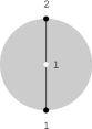
Figure 7: One-loop MHV partition.

For one-loop NMHV we have $J^{1}_{1}=\{j^{a},j^{b},j^{c},j^{d},j^{e}\}$, where $j^{a}$ has $m=3$ (see 8 (a)) and $j^{b}$ to $j^{e}$ have $m=4$ (see 8 (b),(c),(d),(e)), and the integrand is given by the sum of five contributions, Eq. (IV.1.3). This can be straightforwardly continued to higher $k$.

$$\begin{array}[]{ccccc}\parbox[c]{43.362pt}{\includegraphics[scale={0.7}]{One_loop_NMHV_part_a.mps}}&\parbox[c]{43.362pt}{\includegraphics[scale={0.7}]{One_loop_NMHV_part_b.mps}}&\parbox[c]{43.362pt}{\includegraphics[scale={0.7}]{One_loop_NMHV_part_c.mps}}&\parbox[c]{43.362pt}{\includegraphics[scale={0.7}]{One_loop_NMHV_part_d.mps}}&\parbox[c]{43.362pt}{\includegraphics[scale={0.7}]{One_loop_NMHV_part_e.mps}}\\ \\ (a)&(b)&(c)&(d)&(e)\end{array}$$ (54)

Figure 8: One-loop NMHV partitions

Similarly one can continue to higher-loop; for the two-loop MHV diagram the set $J^{2}_{0}$ has elements shown in 10 (plus permutations) with $m=3,4$ which correspond to the MHV diagrams Fig. (9). The diagrams $(a)$ and $(c)$ are those listed in Bullimore:2010pj , but diagram $(b)$ is also a valid partition, though one which of course vanishes under the $\eta$ integration.

$$\begin{array}[]{ccc}\parbox[c]{48.4209pt}{\includegraphics[scale={1.0}]{FigTwoloopMHV1.mps}}{}{}{}{}{}&\parbox[c]{79.497pt}{\includegraphics[scale={1.0}]{FigTwoloopMHV2.mps}}{}{}{}{}{}&\parbox[c]{79.497pt}{\includegraphics[scale={1.0}]{FigTwoloopMHV3.mps}}\\ \\ (a)&(b)&(c)\\ \end{array}$$

Figure 9: Two-loop MHV diagrams

$$\begin{array}[]{ccc}\parbox[c]{43.362pt}{\includegraphics[scale={0.7}]{Two_loop_MHV_part_a.mps}}&\parbox[c]{43.362pt}{\includegraphics[scale={0.7}]{Two_loop_MHV_part_b.mps}}&\parbox[c]{43.362pt}{\includegraphics[scale={0.7}]{Two_loop_MHV_part_c.mps}}\\ \\ (a)&(b)&(c)\end{array}$$ (59)

Figure 10: Two-loop MHV partitions

IV.2.2 Proof

Now we proceed to prove inductively that Eq. (51) satisfies the generalized recursions relations. This provides strong evidence that it is indeed a correct expression for the all-loop integrand.

By assumption Eq. (51) is independent of the $\ast$, and so one again chooses $\ast=n$ for convenience. Taking the difference $\int_{\{l\}}(M^{\prime}_{n,k,l}(1,\ldots,n;\{A,B\}_{\{l\}})-M_{n-1,k,l}(2,\ldots,n;\{A,B\}_{\{l\}})$), where the $l$-fold fermionic and $GL(2)$ integrations have been denoted implicitly, only terms with $i_{1}=2$ survive. Thus we pick out the edge connecting $i_{1}$ to another vertex $v$. There are two possibilities, $v\in X$ and $v\in I$, which we now discuss in turn.

For a partition $j^{\alpha}\in J^{l}_{k}$ with $m$ external legs and with $v=i_{m^{\prime}}~{}(m^{\prime}=2,\ldots,m)$, one can pull out a factor from the set of edges $e_{0}=(i_{1},i_{m^{\prime}})$, corresponding to the invariant $[n,1,2,\widehat{i_{m^{\prime}}-1},i_{m^{\prime}}]$, for each $m^{\prime}$, Fig. (11). This gives rise to the terms

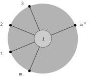
$\Rightarrow$  

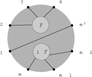
Figure 11: Factorization of loop diagram of type $F$.

$$F=\frac{1}{l!}\sum_{j^{\alpha}\in J^{l}_{k}}\sum^{m}_{m^{\prime}=2}\sum^{n-1}_{i_{m^{\prime}}=4}\int_{\{l\}}\sum_{1<i_{2}\leq\ldots\leq i_{m^{\prime}-1}\leq i_{m^{\prime}}}\sum_{i_{m^{\prime}}\leq i_{m^{\prime}+1}\leq\ldots\leq i_{m}<n}\prod_{e\neq e_{0}}[e]~{},$$ (60)

where we denote the invariants as $[e]=\pm[n,\widehat{v_{1}(e)-1},v_{1}(e),\widehat{v_{2}(e)-1},v_{2}(e)]$.

Now one can rewrite the summation over the partitions for the remaining $k+2l-1$ factors as a summation over $J^{l}_{k-1}(m^{\prime})$, which is defined as the set of all partitions in $J^{l}_{k}$ with $i_{1},i_{m^{\prime}}$ and the edge connecting them removed. By the definition of $J^{l}_{k}$, each partition $j\in J^{l}_{k-1}(m^{\prime})$ splits into two sub-partitions $j_{L}$ and $j_{R}$, both of which are non-crossing partitions. For a partition $j$ with $m$ external legs, the first subpartition, $j_{L}\in J^{l^{\prime}}_{k^{\prime};m^{\prime}-2}$, has $m^{\prime}-2$ external legs while $j_{R}\in J^{l-l^{\prime}}_{k-1-k^{\prime};m-m^{\prime}}$ has $m-m^{\prime}$ external legs. Note that the total number of internal points is $l$, and the total number of edges is $k^{\prime}+2l^{\prime}+(k-1-k^{\prime})+2(l-l^{\prime})=k+2l-1$. Thus every element of $J^{l}_{k-1}(m^{\prime})$, which now includes partitions with arbitrary $m$, is an element of $\cup^{l}_{l^{\prime}=0}\cup^{k-1}_{k^{\prime}=0}J^{l^{\prime}}_{k^{\prime};m^{\prime}-2}\otimes J^{l-l^{\prime}}_{k-1-k^{\prime}}$. Conversely, given any $j_{L}\in J^{l^{\prime}}_{k^{\prime};m^{\prime}-2}$ and $j_{R}\in J^{l-l^{\prime}}_{k-1-k^{\prime}}$, the combined partition $j_{L}\otimes j_{R}$ must be an element of $J^{l}_{k-1}(m^{\prime})$, thus we have the decomposition,

$$J^{l}_{k-1}(m^{\prime})=\cup^{l}_{l^{\prime}=0}\cup^{k-1}_{k^{\prime}=0}J^{l^{\prime}}_{k^{\prime};m^{\prime}-2}\otimes J^{l-l^{\prime}}_{k-1-k^{\prime}},$$ (61)

where we have included all ways of distributing $l$ internal points into two sets of $l^{\prime}$ and $l-l^{\prime}$ points; for a given $k^{\prime}$, no partition exists beyond the range $k^{\prime}+l^{\prime}-f^{\prime}+1\leq m^{\prime}-2\leq 2k^{\prime}+2l^{\prime}-2f^{\prime}+1$ where $f^{\prime}$ and $f-f^{\prime}$ are the numbers of faces in the two partitions respectively.

Now if we relabel the dummy variables, $j=i_{m^{\prime}},m_{L}=m^{\prime}-2,m_{R}=m-m^{\prime}$ and note that $k^{\prime}+l^{\prime}-f^{\prime}+1\leq m_{L}\leq 2k^{\prime}+2l^{\prime}-2f^{\prime}+1$ and $k-k^{\prime}+l-l^{\prime}+f-f^{\prime}\leq m_{R}\leq 2(k-k^{\prime})+2(l-l^{\prime})-2(f-f^{\prime})-1$ for given $k^{\prime},l^{\prime},f^{\prime}$, then by Eq. (61), $F$ splits into the left and the right parts,

$$F=\frac{1}{l!}\sum_{\sigma_{l}}\sum^{n-1}_{j=4}[n,1,2,\widehat{j-1},j]\sum^{k-1}_{k^{\prime}=0}\sum_{j_{L}^{\alpha}\in J^{l^{\prime}}_{k^{\prime}}}\sum_{1<i_{2}\leq\ldots\leq i_{m_{L}+1}\leq j}\int_{\{L\}}\prod_{e\in E(j_{L}^{\alpha})}[e](1,\ldots,j-1,j;\{A,B\}_{L})$$

$$~{}~{}~{}\times\sum_{j_{R}^{\alpha}\in J^{l-l^{\prime}}_{k^{\prime}-1-k^{\prime}}}\sum_{j\leq i_{m_{L}+3}\leq\ldots\leq i_{m_{L}+m_{R}+2}<n}\int_{\{R\}}\prod_{e\in E(j_{R}^{\alpha})}[e](j-1,j,\ldots,n\{A,B\}_{R}),$$ (62)

where $\sigma_{l}$ denotes the summation over all ways of distributing $\{A,B\}_{\{l\}}$ into $\{A,B\}_{L}$ with $l^{\prime}$ points, and $\{A,B\}_{R}$ with $l-l^{\prime}$ points, for $l^{\prime}=0,\ldots,l$, and the integral $\int_{\{l\}}$ splits into $\int_{\{L\}}$ and $\int_{\{R\}}$ correspondingly.

To proceed, we note when $j=i_{m^{\prime}}=i_{m^{\prime}-1}$, a deformation $\widehat{j-1}$ is needed in the factor $[n,1,2,\widehat{j-1},j]$, which is an unwanted feature. However, due to the reversal symmetry as in the tree-level case, one can shift the deformation from $j-1$ in the factor to the last leg $j$ in the left part, which is $(j-1\,j)\cap(n\,1\,2)=I_{j}$ because the other vertex in the preceding edge is $i_{1}=2$. In addition, note that $i_{2}-1$ needs to be deformed when $i_{2}=i_{1}=2$, but, as the first external point in $j_{L}^{\alpha}$, this is not a usual deformation inside the left part, thus can only be achieved by a deformation of its first leg $1$, $\widehat{1}=(1\,2)\cap(n\,j-1\,j)=\hat{1}_{j}$; similarly, the deformation of $i_{m^{\prime}+1}-1$ when $i_{m^{\prime}+1}=i_{m^{\prime}}=j$ is really a deformation on the first leg of the right part, $j-1$, $\widehat{j-1}=(j-1\,j)\cap(n\,1\,2)=I_{j}$. Then by the induction assumption, the left and right parts are given by $M_{j,k^{\prime},l^{\prime}}(\hat{1}_{j},\ldots,j-1,I_{j};\{A,B\}_{L})$ and $M_{n+2-j,k-1-k^{\prime},l-l^{\prime}}(I_{j},j,\ldots,n;\{A,B\}_{R})$, respectively,

$$F = \frac{1}{l!}\sum_{\sigma_{l}}\sum^{n-1}_{j=4}[n,1,2,j-1,j]\Big{[}\sum^{k-1}_{k^{\prime}=0}M_{j,k^{\prime},l^{\prime}}(\hat{1}_{j},\ldots,j-1,I_{j};\{A,B\}_{L})$$ (63)

$$\kern 140.0pt\times M_{n+2-j,k-1-k^{\prime},l-l^{\prime}}(I_{j},j,\ldots,n;\{A,B\}_{R})\Big{]}~{},$$

which, together with $M_{n-1,k,l}$, give exactly the factorization contribution to $M_{n,k,l}$ in the recursion relations.

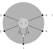
$\Rightarrow$  

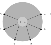
Figure 12: Factorization of loop diagram of type $S$.

The remaining terms are those with $v=A_{l_{0}}(l_{0}=1,\ldots,l)$, which all have a factor $[n,1,2,A_{l_{0}},\widehat{B_{l_{0}}}]$ Fig(12). As we have shown in the one-loop MHV and NMHV cases, for each term one can always redefine the integration variables to shift $\widehat{B_{l_{0}}}$ back to $B_{l_{0}}$ without affecting anything else. For a term to survive the integrations, $A_{l_{0}}$ in the partition should also be connected to (at least one) other vertices $v_{i}$ for $i=1,\ldots,s$. By pulling out the factor and considering the rest as a new partition, one is essentially removing an external point $i_{1}=2$ and an internal point $A_{l_{0}}$, and adding $s$ coinciding external points $v^{\prime}_{i}=A_{l_{0}}$, which are connected to $v_{i}$ for $i=1,\ldots,s$ respectively.

Note that the new partition, which is obviously also non-crossing, has $l-1$ internal points, and $k+2l-1=k+1+2(l-1)$ edges which means it belongs to the $k+1$ sector; the number of faces is $f-s+1\leq f^{\prime}\leq f$, and the number of external points is $m^{\prime}=m+s-1$, which is in the range $k+l-f+s,\ldots,2k+2l-2f+s$. Denote the set of partitions found by pulling $s$ points to the boundary as $J^{l-1}_{k+1}(s)$, this consists of diagrams which have the last $s$ coinciding external points connected to $A_{l_{0}}$. Then the full set of all partitions found by removing a leg connecting an external vertex to an internal vertex, $S^{l}_{k}$ is the union of $J^{l-1}_{k+1}(s)$ for all possible $s$. Conversely taking any element of $S^{l}_{k}$ and joining together the set of legs connected to $A_{l_{0}}$ we find an element of $J^{l-1}_{k+1}(s)$ for some $s$. Thus

$$S^{l}_{k}=\cup_{s}J^{l-1}_{k+1}(s)~{}.$$ (64)

In addition to the summation over $j^{\alpha}\in J^{l-1}_{k+1}(s)$, we also sum over the previous external points, $1<i_{2}\leq\ldots\leq i_{m^{\prime}-s+1}<n$, while constraining the added, last $s$ external points to be fixed at $A_{l_{0}}$, i.e. $i_{m^{\prime}-s+2}=\ldots=i_{m^{\prime}+1}=A_{l_{0}}$, for all possible $s$,

$$S=\frac{1}{l!}\sum^{l}_{l_{0}=1}\int_{\{l\}/l_{0}}\int_{l_{0}}[n,1,2,A_{l_{0}},B_{l_{0}}]\sum_{s}\sum_{j^{\alpha}\in J^{l-1}_{k+1}(s)}\sum_{1<i_{2}\leq\ldots\leq i_{m^{\prime}-s+1}<n}$$

$$\prod_{e\in E(j^{\alpha})}(\pm)[n,\widehat{v_{1}(e)-1},v_{1}(e),\widehat{v_{2}(e)-1},v_{2}(e)]|_{i_{m^{\prime}-s+2}=\ldots=i_{m^{\prime}+1}=A_{l_{0}}},$$ (65)

where the contribution is denoted as $S$. Since we have included all permutations of internal points, any internal point $A_{l_{0}}$ can be connected to $i_{1}=2$, thus there is a summation over $l_{0}$.

Now if we relax the constraints and generally sum over $2\leq i_{2}\leq\ldots\leq i_{m^{\prime}+1}\leq n+2$ with $n+1=B_{l_{0}}$ and $n+2=A_{l_{0}}$, then by splitting the last coinciding $s$ points of any partition in $J^{l-1}_{k+1}(s)\subseteq S^{l}_{k}$, one obtains a partition in $J^{l-1}_{k+1}$; conversely, by joining the last $s$ points of any partition in $J^{l-1}_{k+1}$ for any possible $s$, we obtain either a partition in $J^{l-1}_{k+1}(s)\subseteq S^{l}_{k}$, or a partition with multiple edges connecting the same pair of points, which vanishes immediately. Denoting the set of these bubble diagrams as $B^{l}_{k}$, we have,

$$S^{l}_{k}\cup B^{l}_{k}=J^{l-1}_{k+1}.$$ (66)

By the induction assumption, and note that there is no contribution from $B^{l}_{k}$, then the summations and the integrations $\int_{\{l\}/l_{0}}$, as well as a factor $1/(l-1)!$, give $M_{n+2,k+1,l-1}$,

$$\frac{1}{(l-1)!}\int_{\{l\}/{l_{0}}}\sum_{j^{\alpha}\in J^{l-1}_{k+1}}\sum_{2\leq i_{2}\leq\ldots\leq i_{m^{\prime}+1}\leq n+2}\prod_{e\in E(j^{\alpha})}(\pm)[n,\widehat{v_{1}(e)-1},v_{1}(e),\widehat{v_{2}(e)-1},v_{2}(e)]$$

$$=M_{n+2,k+1,l-1}(\hat{1}_{A_{l_{0}}B_{l_{0}}},\ldots,n,\hat{B_{l_{0}}},A_{l_{0}};\{A,B\}_{\{l\}/{l_{0}}}),$$ (67)

where one needs a deformation on $1$ because the deformation for $i_{2}$ when $i_{2}=i_{1}=2$ is only achieved by always using $\widehat{1}=(1\,2)\cap(n,\,A_{l_{0}}\,B_{l_{0}})=\hat{1}_{A_{l_{0}}B_{l_{0}}}$; also the deformation $\widehat{B_{l_{0}}}=(A_{l_{0}}\,B_{l_{0}})\cap(n\,1\,2)$ is not an usual deformation in $M_{n+2,k+1,l-1}$, thus it is only achieved by always using $\hat{B_{l_{0}}}$, and by the same argument before, all other deformed $B_{l_{0}}$ can be defined by the same deformation acting on $\hat{B_{l_{0}}}$.

By relaxing the constraints, we have included some unwanted terms. Since Eq. (IV.2.2) already has all terms with at least one factor ($s\geq 1$) containing both $A_{l_{0}}$ and $B_{l_{0}}$ (in addition to the prefactor $[n,1,2,A_{l_{0}},B_{l_{0}}]$), as we have shown, all unwanted terms vanish after the integration $\int_{l_{0}}$. Thus we can indeed write the contribution $S$ as an integration of $M_{n+2,k+1,l-1}$,

$$S=\frac{1}{l}\sum^{l}_{l_{0}=1}\int_{l_{0}}[n,1,2,A_{l_{0}},B_{l_{0}}]M_{n+2,k+1,l-1}(\hat{1}_{A_{l_{0}}B_{l_{0}}},\ldots,n,A_{l_{0}},\hat{B}_{l_{0}};\{A,B\}_{\{l\}/{l_{0}}}),$$ (68)

where we have exchanged $A_{l_{0}}$ and $\hat{B}_{l_{0}}$ because in the surviving terms, either order gives the same result. Finally, by combining $F$ from Eq. (63) and the source term $S$ from Eq. (IV.2.2) together,

$$M_{n,k,l}(1,\ldots,n;\{A,B\}_{l})=M_{n-1,k,l}(2,\ldots,n;\{A,B\}_{l})+F+S,$$ (69)

we have seen that Eq. (51) indeed gives an explicit solution to the recursion relations to all loops. This provides strong evidence for the all-loop MHV vertex expansion Eq. (51).

We stress again that the general formula Eq. (51) is completely cyclically invariant and thus it can generate different forms of all-loop integrands by choosing different reference twistors. By considering generalized BCFW relations with different shifts one can see that the expression Eq. (51) is valid for a choice of the reference twistor equal to any of the external twistors. However, this does not prove that the formula is completely independent of the choice of such a reference twistor. It should be possible to prove this by considering all-line shifts as in the standard case.

Figure 13: One-loop NMHV tadpole partition.

Just as we have shown that the MHV diagrams corresponding to the graphs in $J^{l}_{k}$ satisfy a recursion relation, one can similarly derive a recursion relation for the number of graphs. To be specific, let us consider the class of non-crossing graphs described above: with $m$ external points, $l$ internal points, and $k+2l$ edges. We define $C^{l}_{k;m}$ to the number of non-crossing partitions or dual graphs, restricted to graphs with distinct external points, i.e. they all have exactly three adjacent edges, but relaxing the definition to include graphs with internal faces with one or two edges, i.e. bubbles or tadpoles attached to internal vertices, for example $C^{1}_{1;3}$ would now include Fig.(13) in addition to Fig.(8) (a). $C^{l}_{k;m}$ satisfies the recursion relation

$$C^{l}_{k;m} = \sum_{l^{\prime}=0}^{l}\sum_{k^{\prime}=0}^{k-1}\sum_{m^{\prime}=2}^{m}C^{l^{\prime}}_{k^{\prime};m^{\prime}-2}C^{l-l^{\prime}}_{k-k^{\prime}-1;m-m^{\prime}}+\sum_{s=1}^{s_{max}}C^{l-1}_{k+1;m+s-1}$$ (70)

where $s_{max}=1$ if $C^{l}_{k;m}$ has no internal faces, $s_{max}=2$ if $C^{l}_{k;m}$ has one internal face, and $s_{max}=2+f_{max}$ for $f_{max}>1$ where $f_{max}$ is the maximum number of allowed number of faces in $C^{l}_{k;m}$ which is 0 for $l=0$ and $k+l-m+1$ for $l<0$. As a boundary condition, we define $C^{0}_{0;0}=1$.

V Conclusions and Outlook

In this work we have shown that the expressions for the tree-level amplitudes and loop integrands following from the momentum twistor space MHV vertex expansion satisfy the ABCCT recursion relations. This provides strong evidence for the validity of the MHV vertex expansion to all loop order and the independence of the expressions on the choice of reference twistor. Correspondingly, the expressions from the MHV expansion provide manifestly cyclicly invariant solutions of the ABCCT recursion relations.

In BCFW and ABCCT recursion relations, the many important properties of tree amplitudes and loop integrands, such as cyclic-invariance, absence of spurious poles, correspond to a set of highly non-trivial relations between rational functions ArkaniHamed:2009dn . At tree-level, these relations can be understood as arising from the global residue theorem applied to the Grassmannian integral ArkaniHamed:2009dn ; Broedel:2010rr , and generalizations to loop-level have been suggested in ArkaniHamed:2010kv . It would be interesting to see how those relations, or the residue theorem, arise from the explicit solution which unifies different the forms of loop integrands. Furthermore, it is possible to obtain the general local form of integrands for all numbers of legs and all loop orders, generalizing results of ArkaniHamed:2010kv .

Of course one is ultimately interested in the integrated expressions and so a regulator for the IR divergences must be introduced. A convenient choice, which can be implemented in momentum twistor space Hodges:2010kq ; Mason:2010pg , is a mass-regulator which corresponds to higgsing the theory e.g. Alday:2007hr ; Alday:2009zm (see Alday:2010jz ; Drummond:2010mb for recent use of this regulator in explicit calculations). While this regulator is natural from the dual conformal point of view, the full Yangian symmetry, in particular the usual conformal symmetry, is still not well-understood in the presence of IR divergences and naïvely it becomes anomalous. At tree-level it was shown that the superconformal and dual superconformal symmetries, properly understood Bargheer:2009qu , Sever:2009aa , could be used to uniquely fix the tree level amplitudes Bargheer:2009qu . This was equivalent to using the naïve symmetry generators and accounting for the collinear or soft behavior of the amplitudes Korchemsky:2009hm . At loop level it was further shown how to deform the symmetry generators, to account for the anomalous contributions arising from regulator, acting on the full one-loop amplitudes Beisert:2010gn . In that work the amplitudes were all defined using the version of dimensional reduction commonly used in explicit calculations of amplitudes. A related prescription for the symmetry generators, based on an all-loop generalization of the CSW prescription combined with a novel regulator was proposed in Sever:2009aa . Since we have written down all-loop integrands in a concise form, it would be interesting to see if the symmetries, again defined appropriately, can be used to determine these integrands. To extend this to the full all-loop amplitudes it may be useful to reconsider these earlier calculations in the momentum twistor space formulation and with the mass regulator. In a perhaps related direction, differential operators which relate integrals at different loop orders were recently found in momentum twistor space Drummond:2010cz .

In work closely related to the development of the momentum twistor MHV expansion, Mason and Skinner Mason:2010yk showed that the correlations of the Wilson loop in momentum twistor space lead exactly to the MHV expansion for scattering amplitudes but with the diagrams being the planar duals of the MHV diagrams. Another, presumably equivalent or related, proposal for a supersymmetric Wilson loop CaronHuot:2010ek , building on the considerations of Eden:2010zz ; Eden:2010ce , has been shown to satisfy recursion relations equivalent to those of ABCCT at tree and loop level. Relatedly, Brandhuber et al Brandhuber:2010mi presented a set of dual momentum space rules, interpreted as dual momentum space Wilson loop diagrams. These rules are equivalent to the ordinary MHV rules and simply correspond to their dual graph representation. In our work we have introduced non-crossing partitions which are in one-to-one correspondence with the dual MHV graphs. It may be fruitful to understand exactly the relation between all these prescriptions. In particular, the explicit formula we obtained should naturally follow from a dual graph expansion of the Wilson loops.

In demonstrating that the MHV expansion satisfies the ABCCT relations we have made use of the freedom to choose the reference twistor. However, while it is almost certainly true that the expressions are independent of this choice it would be nice to prove it. Our result is valid for a choice of the reference twistor equal to any of the external twistors, since it can be derived from recursion relations by shifting any external twistor. Thus this provides some evidence for the arbitrary nature of the reference twistor. In a very recent paper Bullimore:2010dz , Bullimore adopted a complementary method to show the MHV expansion satisfies recursion relations derived from the momentum-twistor version of the all-line shift Risager:2005vk ; Elvang:2008vz , thus it is at least valid for all reference twistors of the form $\mathcal{Z}_{\ast}=(0,\iota^{\dot{\alpha}},0)$.

It may also be possible to extend these results to wider class of observables such as form factors. The string dual of these observables is also described by an integrable model and their strong coupling value is calculable by a set of equations of the Y-system form Maldacena:2010kp . At weak coupling there is evidence Bork:2010wf of dual conformal symmetry or at least a residue thereof and so they may be expressible in terms of Yangian invariants. It would be interesting to investigate whether recursion relations for these quantities can be found.

Finally, we emphasize that rewriting the MHV expansion in terms of non-crossing partitions has the advantage of systematically organizing all planar MHV diagrams, and yielding more explicit results. As a byproduct, our expressions for the MHV expansion, combined with the ABCCT relations, provide a simple recursive formula for the number of generalized non-crossing partitions or equivalently a particular class of dual planar graphs.

Acknowledgements: We would like to thank G. S. Vartanov for useful conversations and kindly informing us of Bork:2010wf . We are also grateful to M. Bullimore for several insightful comments and questions.

Appendix A Non-crossing partitions and dual diagrams

The non-crossing partitions we have introduced are obviously closely related to the dual graphs of the MHV vertex diagrams composing the amplitude (which have appeared in this context recently in Mason:2010yk ; Brandhuber:2010mi ). Here we attempt to make this relationship clearer and in doing so argue for the validity of our expression Eq. (51). Starting with the simplest tree-level diagram, Fig.(1), we write the MHV vertex as a graph vertex. First we collapse each group of external legs into a single leg ending on a new vertex, and we furthermore identify all these new vertices, see Fig.(14). In general, this produces a (multi)graph on the sphere with faces corresponding to momentum regions. Of course, graphs on a sphere are in one-to-one correspondence with planar graphs (where one of the faces corresponds to the exterior region). For every planar graph one can construct the geometric dual graph, for example Fig.(14), which is seen, in this case, to correspond to the non-crossing partition with the external vertices connected by edges.

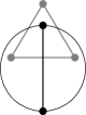
Figure 14: Graph and dual graph for the NMHV diagram.The uppermost point of the graph is the added vertex upon which the external legs end.

While for more complicated tree diagrams the resulting graphs are more involved one can always construct a dual graph in this fashion. Furthermore, the dual of each graph is unique. These planar graphs are always such that each edge ends on two distinct vertices (no pseudographs), and in fact each face is bounded by exactly three edges. This corresponds to assuming that for each location in the original MHV diagram where external legs can occur they do. The case where there are no external legs, for example if $i_{2}=i_{3}$ in Fig.(2), is a degenerate case which corresponds to two vertices becoming coincident in the dual graph. For example in Fig.(15) we show the graph corresponding to the N²MHV diagram, the dual graph, the degenerate graph for $i_{2}=i_{3}$ and its dual.

$$\begin{array}[]{cccc}\parbox[c]{37.5804pt}{\includegraphics[scale={0.7}]{TreeNNMHVgraph.mps}}{}{}&\parbox[c]{28.908pt}{\includegraphics[scale={0.7}]{TreeNNMHVdgraph.mps}}{}{}&\parbox[c]{25.2945pt}{\includegraphics[scale={0.7}]{TreeNNMHVgraphdegen.mps}}{}{}&\parbox[c]{28.908pt}{\includegraphics[scale={0.7}]{TreeNNMHVdgraphdegen.mps}}\\ (a){}{}&(b){}{}&(c){}{}&(d){}{}\end{array}$$ (72)

Figure 15: Tree N²MHV graph (a), the dual graph (b), the degenerate N²MHV graph (c) and the dual of the degenerate graph.

Furthermore, before identifying the end vertices there are no cycles, thus after the identification every cycle must include the added vertex corresponding to the identified ends of all external legs. That is to say, the graphs are such that every cycle has at least one vertex in common. For the dual diagrams this implies that every vertex is connected to at least three edges and there is one face (in our embedding this is the exterior region) such that every cut set

$$\begin{array}[]{ccc}\parbox[c]{44.0847pt}{\includegraphics[scale={1}]{Treecutdgraph.mps}}{}{}&\parbox[c]{37.5804pt}{\includegraphics[scale={1}]{Loopcutdgraph_a.mps}}{}{}&\parbox[c]{37.5804pt}{\includegraphics[scale={1}]{Loopcutdgraph_b.mps}}\\ (a){}{}&(b){}{}&(c)\end{array}$$ (74)

Figure 16: (a) Cut for a dual tree graph (b) Boundary cut for a dual graph (c) Loop cut for a dual graph

must contain two edges of the boundary of that face e.g. Fig.(16) (a). In the degenerate graphs vertices can come together, in which case one could have more than three edges attached to a vertex.

Figure 17: Graph and dual graph for the one-loop MHV diagram.

Now we consider MHV diagrams with loops, the simplest example of which, the one loop MHV diagram, is shown in Fig.(17). As can be seen even in this simplest case, for the MHV diagrams we must include faces corresponding to loops which in general can have more than three boundary edges; we thus have two classes of faces. As we do not consider tadpoles, as they give zero after fermionic integration, those faces corresponding to loops must have at least two edges each. In fact, graphs where an internal face has only two edges but shares one of its edges with another loop will also give zero contribution to the MHV expansion after the fermionic integration. This is the case, for example, in the two loop MHV diagrams Fig.(9) (b). Contrary to the tree level graphs, there are now, of course, completely disjoint cycles.

For the corresponding dual diagrams we thus have two types of vertices, which we represent with black dots for vertices dual to faces corresponding to external momenta and white dots for vertices dual to faces corresponding to loop momenta. Black dots must always have three adjacent edges and white dots at least two edges. In fact, for the purposes of integrands, white dots must have two edges each, that is they cannot each have only two edges but share an edge. Every face must have a boundary consisting of at least three edges. Finally, there is a face (in our representations this will be the exterior face) such that the cut sets of cuts that result in two partitions both consisting of mixes of white and black vertices must contain elements of the boundary of this face e.g. Fig.(16) (b). The cut sets of cuts which result in partitions one of which contains only white vertices contain no elements of the boundary of this face e.g. Fig.(16) (c). These cuts correspond to the cycles introduced by the loops.

The partitions described earlier can be found by eliminating the boundary of the preferred, or exterior face. This gives us a one-to-one mapping between MHV diagrams, their graphs, their duals and the corresponding partitions.

References

- (1) F. Cachazo, P. Svrcek and E. Witten, “MHV vertices and tree amplitudes in gauge theory”, JHEP 0409, 006 (2004), hep-th/0403047.
- (2) E. Witten, “Perturbative gauge theory as a string theory in twistor space”, Commun. Math. Phys. 252, 189 (2004), hep-th/0312171.
- (3) A. Brandhuber, B. J. Spence and G. Travaglini, “One-loop gauge theory amplitudes in N=4 super Yang-Mills from MHV vertices”, Nucl.Phys. B706, 150 (2005), hep-th/0407214.
- (4) A. Gorsky and A. Rosly, “From Yang-Mills Lagrangian to MHV diagrams”, JHEP 0601, 101 (2006), hep-th/0510111.
- (5) P. Mansfield, “The Lagrangian origin of MHV rules”, JHEP 0603, 037 (2006), hep-th/0511264.
- (6) J. H. Ettle and T. R. Morris, “Structure of the MHV-rules Lagrangian”, JHEP 0608, 003 (2006), hep-th/0605121, Makes major improvements on withdrawn paper hep-th/0605024.
- (7) R. Boels, L. Mason and D. Skinner, “From twistor actions to MHV diagrams”, Phys.Lett. B648, 90 (2007), hep-th/0702035.
- (8) R. Britto, F. Cachazo and B. Feng, “New recursion relations for tree amplitudes of gluons”, Nucl. Phys. B715, 499 (2005), hep-th/0412308.
- (9) R. Britto, F. Cachazo, B. Feng and E. Witten, “Direct proof of tree-level recursion relation in Yang-Mills theory”, Phys. Rev. Lett. 94, 181602 (2005), hep-th/0501052.
- (10) J. M. Drummond and J. M. Henn, “All tree-level amplitudes in 4 SYM”, JHEP 0904, 018 (2009), 0808.2475.
- (11) K. Risager, “A Direct proof of the CSW rules”, JHEP 0512, 003 (2005), hep-th/0508206.
- (12) H. Elvang, D. Z. Freedman and M. Kiermaier, “Proof of the MHV vertex expansion for all tree amplitudes in N=4 SYM theory”, JHEP 0906, 068 (2009), arXiv:0811.3624.
- (13) A. Brandhuber, P. Heslop and G. Travaglini, “A note on dual superconformal symmetry of the 4 super Yang-Mills S-matrix”, Phys. Rev. D78, 125005 (2008), 0807.4097.
- (14) J. M. Drummond, J. Henn, V. A. Smirnov and E. Sokatchev, “Magic identities for conformal four-point integrals”, JHEP 0701, 064 (2007), hep-th/0607160.
- (15) J. M. Drummond, J. Henn, G. P. Korchemsky and E. Sokatchev, “Dual superconformal symmetry of scattering amplitudes in 4 super-Yang–Mills theory”, 0807.1095.
- (16) J. M. Drummond, J. M. Henn and J. Plefka, “Yangian symmetry of scattering amplitudes in 4 super Yang-Mills theory”, JHEP 0905, 046 (2009), 0902.2987.
- (17) A. Hodges, “Eliminating spurious poles from gauge-theoretic amplitudes”, 0905.1473.
- (18) N. Arkani-Hamed, F. Cachazo, C. Cheung and J. Kaplan, “A Duality For The S Matrix”, JHEP 1003, 020 (2010), arXiv:0907.5418, * Temporary entry *.
- (19) L. Mason and D. Skinner, “Dual Superconformal Invariance, Momentum Twistors and Grassmannians”, JHEP 0911, 045 (2009), arXiv:0909.0250.
- (20) J. Drummond and L. Ferro, “Yangians, Grassmannians and T-duality”, JHEP 1007, 027 (2010), arXiv:1001.3348.
- (21) G. Korchemsky and E. Sokatchev, “Superconformal invariants for scattering amplitudes in N=4 SYM theory”, Nucl.Phys. B839, 377 (2010), arXiv:1002.4625, * Temporary entry *.
- (22) J. Drummond and L. Ferro, “The Yangian origin of the Grassmannian integral”, arXiv:1002.4622, * Temporary entry *.
- (23) N. Arkani-Hamed, J. L. Bourjaily, F. Cachazo, S. Caron-Huot and J. Trnka, “The All-Loop Integrand For Scattering Amplitudes in Planar N=4 SYM”, arXiv:1008.2958.
- (24) R. H. Boels, “On BCFW shifts of integrands and integrals”, arXiv:1008.3101.
- (25) M. Bullimore, L. Mason and D. Skinner, “MHV Diagrams in Momentum Twistor Space”, arXiv:1009.1854, * Temporary entry *.
- (26) R. P. Stanley, “Enumerative Combinatorics, Volume 2, Catalan appendum”, Cambridge University Press ( 2001).
- (27) L. Mason and D. Skinner, “The Complete Planar S-matrix of N=4 SYM as a Wilson Loop in Twistor Space”, arXiv:1009.2225, * Temporary entry *.
- (28) S. Caron-Huot, “Notes on the scattering amplitude / Wilson loop duality”, arXiv:1010.1167, * Temporary entry *.
- (29) A. Brandhuber, B. Spence, G. Travaglini and G. Yang, “A Note on Dual MHV Diagrams in N=4 SYM”, arXiv:1010.1498, * Temporary entry *.
- (30) J. Brodel and S. He, “Dual conformal constraints and infrared equations from global residue theorems in N=4 SYM theory”, JHEP 1006, 054 (2010), 1004.2400.
- (31) A. Hodges, “The box integrals in momentum-twistor geometry”, arXiv:1004.3323, * Temporary entry *.
- (32) L. Mason and D. Skinner, “Amplitudes at Weak Coupling as Polytopes in AdS5”, arXiv:1004.3498, * Temporary entry *.
- (33) L. F. Alday and J. M. Maldacena, “Gluon scattering amplitudes at strong coupling”, JHEP 0706, 064 (2007), 0705.0303.
- (34) L. F. Alday, J. M. Henn, J. Plefka and T. Schuster, “Scattering into the fifth dimension of N=4 super Yang- Mills”, 0908.0684.
- (35) L. F. Alday, “Some analytic results for two-loop scattering amplitudes”, arXiv:1009.1110, * Temporary entry *.
- (36) J. M. Drummond and J. M. Henn, “Simple loop integrals and amplitudes in N=4 SYM”, arXiv:1008.2965.
- (37) T. Bargheer, N. Beisert, W. Galleas, F. Loebbert and T. McLoughlin, “Exacting 4 Superconformal Symmetry”, 0905.3738.
- (38) A. Sever and P. Vieira, “Symmetries of the 4 SYM S-matrix”, 0908.2437.
- (39) G. P. Korchemsky and E. Sokatchev, “Symmetries and analytic properties of scattering amplitudes in 4 SYM theory”, 0906.1737.
- (40) N. Beisert, J. Henn, T. McLoughlin and J. Plefka, “One-Loop Superconformal and Yangian Symmetries of Scattering Amplitudes in N=4 Super Yang-Mills”, JHEP 1004, 085 (2010), arXiv:1002.1733.
- (41) J. M. Drummond, J. M. Henn and J. Trnka, “New differential equations for on-shell loop integrals”, arXiv:1010.3679, * Temporary entry *.
- (42) B. Eden, G. P. Korchemsky and E. Sokatchev, “From correlation functions to scattering amplitudes”, arXiv:1007.3246.
- (43) B. Eden, G. P. Korchemsky and E. Sokatchev, “More on the duality correlators/amplitudes”, arXiv:1009.2488, * Temporary entry *.
- (44) M. Bullimore, “MHV Diagrams from an All-Line Recursion Relation”, 1010.5921, * Temporary entry *.
- (45) J. Maldacena and A. Zhiboedov, “Form factors at strong coupling via a Y-system”, arXiv:1009.1139, * Temporary entry *.
- (46) L. Bork, D. Kazakov and G. Vartanov, “On form factors in N=4 sym”, 1011.2440, * Temporary entry *.