An extended scaling analysis of the $S=1/2$ Ising ferromagnet on the simple cubic lattice

Abstract

It is often assumed that for treating numerical (or experimental) data on continuous transitions the formal analysis derived from the renormalization group theory can only be applied over a narrow temperature range, the ”critical region”; outside this region correction terms proliferate rendering attempts to apply the formalism hopeless. This pessimistic conclusion follows largely from a choice of scaling variables and scaling expressions which is traditional but very inefficient for data covering wide temperature ranges. An alternative ”extended scaling” approach can be made where the choice of scaling variables and scaling expressions is rationalized in the light of well established high temperature series expansion developments. We present the extended scaling approach in detail, and outline the numerical technique used to study the three-dimensional $3$d Ising model. After a discussion of the exact expressions for the historic $1$d Ising spin chain model as an illustration, an exhaustive analysis of high quality numerical data on the canonical simple cubic lattice $3$d Ising model is given. It is shown that in both models, with appropriate scaling variables and scaling expressions (in which leading correction terms are taken into account where necessary), critical behavior extends from $T_{c}$ up to infinite temperature.

I Introduction

Understanding the universal critical behavior observed at and near continuous transitions is one of the major achievements of statistical physics; the subject has been studied in depth for many years. It is generally considered however that the formalism based on the elegant renormalization group theory (RGT) can only be applied over a narrow temperature range, the ”critical region”, while outside this region correction terms proliferate so attempts to extend the analysis become pointless. In fact this pessimistic conclusion follows largely because the traditional choices of scaling variables and scaling expressions are poorly adapted to the study of wide temperature ranges.

The expressions for critical divergencies of observables $Q(T)$ near a critical temperature $T_{c}$ and in the thermodynamic (infinite size) limit are conventionally written

$$Q(T)=C_{Q}t^{-q}\left(1+F_{Q}(t)\right)$$ (1)

with the scaling variable $t$ defined as

$$t=(T-T_{c})/T_{c}$$ (2)

and where $F_{Q}(t)$ represents an infinite set of confluent and analytic correction terms wegner:72

$$F_{Q}(t)=a_{Q}t^{\theta}+b_{Q}t+\cdots$$ (3)

The exponents q, the confluent correction exponent $\theta$, and many critical parameters such as amplitude ratios and finite size scaling functions, are universal, i.e. they are identical for all members of a universality class of systems. When the RGT formalism is outlined in textbooks or in authoritative reviews such as those of Privman, Hohenberg and Aharony privman:91 or Pelissetto and Vicari pelissetto:02 the scaling variable is defined as $t$ from the outset. However, because $t\to\infty$ at infinite temperature, when $t$ is chosen as the scaling variable the correction terms in $F_{Q}(t)$ each individually diverge as temperature is increased. It indeed becomes extremely awkward to use the expressions in Eq.(3) outside a narrow ”critical” temperature region. A ”critical-to-classical crossover” has been invoked (e.g. Refs. luijten:97 ; garrabos:06 ) with the effective exponent $\gamma_{\mathrm{eff}}(\beta)$ tending to the mean field values as the high temperature Gaussian fixed point is approached. The crossover appears as a consequence of the definition of the exponent in terms of the thermodynamic susceptibility and the scaling variable $t$. There is no such crossover when the extended scaling analysis described below is used.

Although this is rarely stated explicitly, there is nothing sacred about the scaling variable $t$; alternative scaling variables $\tau$ can be legitimately chosen and indeed have been widely used in practice, see e.g. Refs. fahnle:84 ; gartenhaus:88 ; kim:96 ; butera:02 ; deng:03 ; caselle:97 .

Temperature dependent prefactors can also be introduced in the scaling expressions on condition that the prefactor does not have a critical temperature dependence at $T_{c}$.

An ”extended scaling” approach campbell:06 ; campbell:07 ; campbell:08 ; katzgraber:08 ; hukushima:09 has been introduced which consists in a simple systematic rule for selecting scaling variables and prefactors, inspired by the well established high temperature series expansion (HTSE) method. This approach is a rationalization which leads automatically to well behaved high temperature limits as well as giving the correct critical limit behavior.

Here we give a general discussion of this approach. We outline the relationship to the RGT scaling field formalism. As an illustration of the application of the rules, known analytic results on the historically important $S=1/2$ Ising ferromagnet chain in dimension one (for which the critical temperature is of course $T_{c}=0$) are cited. Simple extended scaling expressions for the reduced susceptibility, the second moment correlation length, and the specific heat are exact over the entire temperature range from zero to infinity. An exact susceptibility finite size scaling function is exhibited.

The $S=1/2$ nearest neighbor Ising ferromagnet on the simple cubic lattice is then discussed in detail. This model is among the principal canonical examples of a system having a continuous phase transition at a non-zero critical temperature. In contrast to the two-dimensional $2$d Ising model, in three dimensions no exact values are known for the critical temperature or the critical exponents. We analyze high quality large scale numerical data which have been obtained for sizes up to $L=256$, covering wide temperature ranges both above and below the critical temperature haggkvist:04 ; haggkvist:07 . The numerical technique is outlined. An analysis using the extended scaling approach provides compact critical expressions with a minimum of correction terms, which are accurate (if not formally exact) over the entire temperature range from $T_{c}$ to infinity and not only within a narrow critical regime. (The $3$d Ising, XY, and Heisenberg ferromagnets have been discussed in Ref. campbell:07 ).

II Definitions of variables

We study the $S=1/2$ nearest neighbor interaction ferromagnetic Ising model on the $1$d chain and on the simple cubic lattices of size $L^{3}$ with periodic boundary conditions. The Hamiltonian with nearest neighbor interactions of strength $J$ is

$$\mathcal{H}=-J\sum_{ij}S_{i}\cdot S{j}$$ (4)

with the sum over nearest neighbor bonds. As usual we will use throughout the normalized inverse temperature $\beta\equiv J/kT$.

The observables we have studied are as follows:

(i) The variance of the equilibrium sample moment, which is equal to the non-connected reduced susceptibility

$$\chi(\beta,L)=N\,\langle m^{2}\rangle=(1/N)\,\sum_{i,j}\langle S_{i}\cdot S{j}\rangle$$ (5)

where $m$ is the magnetization per spin $m=(1/N)\sum_{i}S_{i}$, $N=L^{d}$.

(ii) The variance of the modulus of the equilibrium sample moment, or the ”modulus susceptibility”

$$\chi_{\mathrm{mod}}(\beta,L)=N\left(\langle m^{2}\rangle-\langle|m|\rangle^{2}\right)$$ (6)

Below $T_{c}$, $\chi_{\mathrm{mod}}(\beta,L)$ tends to the connected reduced susceptibility in the thermodynamic limit, and

$$\langle|m|\rangle(\beta,L)=\sqrt{\chi(\beta,L)-\chi_{\mathrm{mod}}(\beta,L)}/\sqrt{N}$$ (7)

tends to the thermodynamic limit magnetization $\langle m\rangle(\beta,L)$ at large $L$.

(iii) The specific heat which is equal to the variance of the energy per spin $U(\beta,L)$

$$C_{v}(\beta,L)=N\,\left(\langle U^{2}\rangle-\langle U\rangle^{2}\right)$$ (8)

where U = $(1/N)\,\sum_{ij}S_{i}\cdot S_{j}$ with the sum over nearest neighbor bonds. We can note that $\chi(\beta)$ and $C_{v}(\beta)$ have consistent statistical definitions in terms of thermal fluctuations. The experimentally observed susceptibility contains an extraneous factor $\beta$.

The thermodynamic limit second moment correlation length is defined fisher:67 ; butera:02 by

$$\xi^{2}(\beta,\infty)=\mu_{2}(\beta,\infty)/2d\chi(\beta,\infty)$$ (9)

where the second moment of the correlation function is

$$\mu_{2}(\beta,\infty)=(1/N)\sum_{i,j}\langle r_{i,j}^{2}S_{i}\cdot S_{j}\rangle$$ (10)

with $r_{i,j}$ the distance between spins $i$ and $j$, summing to infinity.

When the ”thermodynamic limit” condition $L\gg\xi(\beta,\infty)$ holds all properties become independent of $L$ and so are identical to the thermodynamic limit properties.

For general $L$, the Privman-Fisher finite size scaling ansatz for an observable $Q$ can be written brezin:82 ; calabrese:03

$$Q(\beta,L)/Q(\beta,\infty)=$$ (11)

$$F_{Q}\left(L/\xi(\beta,\infty)\right) \left(1+L^{-\omega}G_{Q}\left(L/\xi(\beta,\infty)\right)\right)$$

The functions $F_{Q}\left(x\right)$, $G_{Q}\left(x\right)$ are universal. $F_{\chi}\left(x\right)$ must tend to $1$ when $x\gg 1$, and must be proportional to $x^{2-\eta}$ when $x\ll 1$. We are aware of no generally accepted explicit expressions for $F_{Q}\left(x\right)$ valid over the entire range of $x$.

III Extended scaling

In the extended scaling approach campbell:06 ; campbell:07 a systematic choice of scaling variables and scaling expression prefactors is made in the light of the HTSE. Basically, an ideal HTSE corresponds to the power series

$$(1-y)^{-q}\equiv 1+qy+(q(q+1)/2)y^{2}+\cdots$$ (12)

When a real physical HTSE has the form

$$Q\left(x\right)=C_{Q}\,\left(1+a_{1}x+a_{2}x^{2}+\cdots\right)$$ (13)

with a general structure similar to but not strictly equivalent to that of Eq.(12) and a prefactor $C_{Q}$ which can be temperature dependent, the asymptotic limit is eventually dominated by the closest singularity to the origin (Darboux’s first theorem darboux:78 ) leading to the critical limit $Q(x)=C_{Q}(1-x)^{-q}$. The appropriate critical scaling variable is $1-x$, and deviations of the series in Eq.(13) from the pure Eq.(12) form correspond to confluent and analytic critical correction terms.

The extended scaling prescription consists in identifying scaling variables and prefactors such that each series is transposed to a form having the same structure as Eq.(13), with the prefactor defined so that the first term of the series is equal to $1$.

The HTSE spin $S=1/2$ expressions for the reduced susceptibility and the second moment of the correlation can be written generically in the form fisher:67 ; butera:02 ; butera:lib

$$\chi(\beta)=1+a_{1}x+a_{2}x^{2}+a_{3}x^{3}+\cdots$$ (14)

and

$$\mu_{2}(\beta)=b_{1}x+b_{2}x^{2}+b_{3}x^{3}+\cdots$$ (15)

where $x$ is a normalized variable which tends to $1$ as $\beta\to\beta_{c}$ and to zero when $\beta\to 0$.

For ferromagnets, (e.g. fisher:67 ; butera:02 ; butera:lib ) possible natural choices for $x$ are $x=\beta/\beta_{c}$ or $x=\tanh\beta/\tanh\beta_{c}$. Scaling variables for $\chi(\beta)$ are $\tau=1-x=1-\beta/\beta_{c}$ or $\tau=1-x=1-\tanh\beta/\tanh\beta_{c}$. The former is standard when $T_{c}$ is non-zero; when $T_{c}=0$, it is convenient to use $x=\tanh\beta$ (as $\beta_{c}=\infty$, $\tanh\beta_{c}=1$).

For $\mu_{2}(\beta)$ the Eq.(13) form with the same $x$ can be retrieved by extracting a temperature dependent prefactor $b_{1}x$ so as to write

$$\mu_{2}(\beta)=b_{1}x(1+(b_{2}/b_{1})x+(b_{3}/b_{1})x^{2}+\cdots)$$ (16)

The critical expressions for the reduced susceptibility and the second moment correlation length can then be written

$$\chi(\beta,\infty)=C_{\chi}\tau^{-\gamma}\left(1+F_{\chi}(\tau)\right)$$ (17)

(c.f. Eq.(1)) and from the relation Eq.(9) between $\mu_{2}$ and $\xi$,

$$\xi(\beta,\infty)=C_{\xi}x^{1/2}\tau^{-\nu}\left(1+F_{\xi}(\tau)\right)$$ (18)

with the temperature scaling variable $\tau=1-x$ and the standard definitions for the critical amplitudes $C_{\chi}$ and $C_{\xi}$. The $\chi(\beta,\infty)$ expression has been widely used; the $\xi(\beta,\infty)$ expression is specific to the extended scaling approach campbell:06 ; campbell:07 . The $F$ functions contain all the confluent and analytic correction to scaling terms wegner:72 ; wegner:76

$$F_{Q}(\tau)=a_{Q}\tau^{\theta}+b_{Q}\tau+\cdots$$ (19)

It is important that $\tau$ tends to $1$ at infinite temperature (whereas $t$ tends to infinity); the $F_{Q}(\tau)$ thus remain well behaved over the entire temperature range. There are exact closure conditions for the infinite temperature limit $\tau\to 1$ : $C_{\chi}(1+F_{\chi}(1))=1$ and $C_{\xi}/\beta_{c}^{1/2}(1+F_{\xi}(1))=1$ (or $C_{\xi}/(\tanh\beta_{c})^{1/2}(1+F_{\xi}(1))=1$).

One can define temperature dependent effective exponents (introduced by kouvel:64 ):

$$\gamma_{\mathrm{eff}}(\tau)=\partial{\log\chi(\beta)}/\partial{\log\tau}$$ (20)

see Refs. orkoulas:00 ; butera:02 . For the correlation length,

$$\nu_{\mathrm{eff}}(\tau)=\partial{\log(\xi(\beta)/\beta^{1/2})}/\partial{\log\tau}$$ (21)

is the extended scaling definition for $\nu_{\mathrm{eff}}$.

For a spin $S=1/2$ Ising ferromagnet on a lattice where each spin has $z$ neighbors, the high temperature limit of the effective exponents defined by Eqns. 20 and 21 are $\gamma_{\mathrm{eff}}(1)=z\beta_{c}$ and $\nu_{\mathrm{eff}}(1)=\gamma_{\mathrm{eff}}(1)/2$. A comparison between these values and the critical exponents $\gamma$ and $\nu$ gives a good indication of the overall influence of the correction terms. If the leading confluent correction term in Eq.(19) dominates then $\gamma_{\mathrm{eff}}(1)-\gamma\approx a_{\chi}\theta$, and $\nu_{\mathrm{eff}}(1)-\nu\approx a_{\xi}\theta$. An analysis along these lines of $\gamma_{\mathrm{eff}}$ for Ising systems with large $z$ was sketched out in Ref.orkoulas:00 . The case of general $S$ is discussed in Appendix A. For all near neighbor Ising ferromagnets on sc or bcc lattices covering the entire range of spin values $S=1/2$ to $S=\infty$ (which are all in the same $3$d universality class), see Ref. butera:02 , $\gamma_{\mathrm{eff}}(1)$ and $\nu_{\mathrm{eff}}(1)$ differ from the critical $\gamma$ and $\nu$ by a few percent at most. For both observables, the total sum of the correction terms is weak over the entire temperature range.

It should be noted that traditional and widely used finite size scaling expressions

$$Q(\beta,L)/L^{q/\nu}=F_{Q}\left(L^{1/\nu}(T-T_{c})/T_{c}\right)$$ (22)

assume implicitly scaling with the scaling variable $t$. As a general rule these expressions should not be used except in the limit of temperatures very close to $T_{c}$; they rapidly becomes misleading and can suggest incorrect values of the exponent $\nu$ if global fits are made to data covering a wider range of temperatures. The extended scaling FSS expressions campbell:06

$$Q(\beta,L)/(LT^{1/2})^{q/\nu}=F_{Q}\left((LT^{1/2})^{1/\nu}(T-T_{c})/T\right)$$ (23)

are valid at all temperatures above $T_{c}$ to within the weak corrections to scaling.

For spin $S=1/2$ Ising spins on a bipartite lattice (such as the $1$d and $3$d sc lattices we will discuss below) there are only even terms in the HTSE for the specific heat butera:02 ; butera:lib

$$C_{v}(\beta)=1+d_{1}x^{2}+d_{2}x^{4}+d_{3}x^{6}+\cdots$$ (24)

A natural scaling expression for the specific heat is

$$C_{v}(\beta)=C_{0}+C_{c}\left(1-x^{2}\right)^{-\alpha}\left(1+F_{c}(1-x^{2})\right)$$ (25)

The constant term $C_{0}$ is present in standard analyses and plays an important rôle in $3$d ferromagnets because the exponent $\alpha$ is small. The extended scaling expression Eq.(25) is not orthodox as it uses a scaling variable, $\tau_{2}=1-x^{2}=\tau(2-\tau)$, which is not the same as the $\tau=1-x$ used as scaling variable for $\chi(\beta)$ and $\xi(\beta)$.

IV Analytic results in one dimension

The original Ising ferromagnet ising:25 consists of a system of $S=1/2$ spins with nearest neighbor ferromagnetic interactions on a one dimensional chain. Because analytic results exist for many of the statistical properties of this system, it is often used as a ”textbook” model in introductions to critical behavior. We will use it to illustrate the extended scaling approach (see Ref. katzgraber:08 ).

The model orders only at $T=0$ (Ref. ising:25 ); when $T_{c}=0$ the critical exponents depend on the choice of the scaling variable. Baxter baxter:82 states : ”[in one dimension] it is more sensible to replace $t=(T-T_{c})/T_{c}$ by $t=\exp(-2\beta)$”; with this scaling variable the exponents are $\gamma=1,\nu=1,\alpha=-1$ [$\alpha=-\nu d$ when $T_{c}=0$ Ref. baker:75 ].

Expressions for $\xi(\beta)$ and $\chi(\beta)$ in the infinite-size limit are readily calculated following standard HTSE rules (see e.g. Ref. fisher:67 ). The reduced susceptibility HTSE can be written as

$$\chi(\beta)=1+2(\tanh\beta+\tanh^{2}\beta+\tanh^{3}\beta+\ldots)$$ (26)

and the HTSE for the second-moment of the correlation is

$$\mu_{2}(\beta)=2(\tanh\beta+2^{2}\tanh^{2}\beta+3^{2}\tanh^{3}\beta+\ldots)$$ (27)

The second-moment correlation length is then given by Eq. (9) with $z=2$. Using the power series sums

$$\sum_{n=1}^{\infty}y^{n}=\frac{y}{(1-y)}$$ (28)

and

$$\sum_{n=1}^{\infty}n^{2}y^{n}=\frac{y(y+1)}{(1-y)^{3}}$$ (29)

the exact expressions for reduced susceptibility and correlation length are thus

$$\chi(\beta)=\exp(2\beta)$$ (30)

and

$$\xi(\beta) = \frac{1}{2}\left(\exp(4\beta)-1\right)^{1/2}$$

(It can be noted that the ”true” correlation length is $\xi_{\mathrm{true}}=-1/\log(\tanh\beta)$. The two correlation lengths are essentially identical for $\beta>2.5$ but are quite different at higher temperatures.)

The internal energy per spin is just

$$U(\beta)=\tanh\beta$$ (32)

so the specific heat

$$C_{v}(\beta)=\cosh^{-2}\beta$$ (33)

Though not immediately recognizable these can all be re-written in precisely the form of the extended scaling Eqns. 17,18,25, with the choice $x=\tanh\beta$ so $\tau=(1-\tanh\beta)$;

$$\chi(\beta)=2(1-\tanh\beta)^{-1}\left(1-(1/2)(1-\tanh\beta)\right)$$ (34)

$$\xi(\beta)=\frac{\tanh^{1/2}\beta}{1-\tanh\beta}$$ (35)

and

$$C_{v}(\beta,\infty)=(1-\tanh^{2}\beta)$$ (36)

and so with the same critical exponents $\gamma=1$, $\nu=1$, $\alpha=-1$ together with critical amplitudes $C_{\chi}=2$, $C_{\xi}=1$, $C_{v}=1$, $C_{0}=0$. There are no analytic corrections to $\xi(\beta)$ or to $C_{v}(\beta)$ and there is only a single simple analytic correction to $\chi(\beta)$. There are no confluent corrections. Note again that these expressions are valid for the entire temperature range from $T=0$ to $T=\infty$.

The finite size scaling function can also be considered. With periodic boundary conditions the finite size reduced susceptibility for a $1$d sample of size $L$ is

$$\chi(\beta,L)=\exp(2\beta)\frac{1-\tanh^{L}\beta}{1+\tanh^{L}\beta}$$ (37)

The finite size scaling function is

$$\chi(\beta,L)/\chi(\beta,\infty)~{}~{}~{}~{}~{}~{}~{}~{}~{}~{}~{}~{}$$ (38)

$$=\tanh(L/2\xi(\beta,\infty))(1+L^{-2}G_{\chi}\left(L/2\xi(\beta,\infty)\right)$$

The simple principle expression

$$F_{\chi}(L/\xi(\beta,\infty))=\tanh(L/2\xi(\beta,\infty))$$ (39)

is exact.

The higher order term $G_{\chi}(x)$ in Eq.(IV) is numerically tiny even for small $L$. We have not found an analytic expression but it can be fitted rather accurately by

$$G_{\chi}(x)=0.168x^{2}\left(1+\tanh(-0.565x^{1.18})\right)$$ (40)

V High dimension limit

For the Ising ferromagnet in the high dimension hypercubic lattice limit $d\to\infty$, with $\tau(\beta)=1-\beta/\beta_{c}$ the reduced susceptibility and the correlation length are

$$\chi(\beta,\infty)\equiv\tau^{-1}$$ (41)

and

$$\xi(\beta,\infty)\equiv(\beta/\beta_{c})^{1/2}\tau^{-1/2}$$ (42)

exactly over the entire temperature range above $T_{c}$; the exponents $\gamma=1,\nu=1/2$ are of course the mean field exponents. These expressions again follow the extended scaling form given above Eqns. 17,18 including the square root prefactor in $\xi(\beta,\infty)$, with no correction terms.

In this high dimension limit the specific heat above $T_{c}$ is zero ($\alpha=0$).

In dimensions above the upper critical dimension but not in the extreme high dimension limit the extended scaling approach has been used successfully to identify the main correction terms in the reduced susceptibility berche:08 .

Thus analytic expressions for models both in the low ($1$d) and high ($d\to\infty$) dimension limits follow the extended scaling forms. This reinforces the argument that these forms can be considered to be generic and should be used at leading order also for intermediate dimensions, where confluent correction terms and small analytic correction terms must be allowed for.

In practice (e.g. Refs. deng:03 ; kim:96 ; gartenhaus:88 ; caselle:97 ; orkoulas:00 ) analyses of $\chi(\beta)$ have long been carried out using $\tau$ as the scaling variable rather than $t$. There are analogous advantages in scaling $\xi(\beta)$ with Eq.(18), which contains the generic $(\beta/\beta_{c})^{1/2}$ (or $(\tanh\beta/\tanh\beta_{c})^{1/2}$) prefactor. We suggest that this form of scaling expression for $\xi(\beta)$ could profitably become equally standard.

VI RGT formalism and extended scaling

In the standard RGT finite size scaling formalism privman:91 ; pelissetto:02 the free energy is written

$$\mathcal{F}(\beta,h,L)=\mathcal{F}_{\mathrm{sing}}(\beta,h,L)+\mathcal{F}_{\mathrm{reg}}(\beta,h,L)$$ (43)

where the singular part encodes the critical behavior and the regular part is practically $L$ independent. Then

$$\mathcal{F}_{\mathrm{sing}}=L^{-d}F\left(u_{h}L^{(d+2-\eta)/2},u_{t}L^{1/\nu}\right)+$$ (44)

$$v_{\omega}L^{-(d+\omega)}F_{\omega}\left(u_{h}L^{(d+2-\eta)/2},u_{t}L^{1/\nu}\right)+\cdots$$

with the scaling fields $u_{h}$ and $u_{t}$ having temperature dependencies

$$u_{h}=ha_{h}(1+a_{1}t+a_{2}t^{2}...)$$ (45)

and

$$u_{t}=t(1+c_{1}t+c_{2}t^{2}+...)$$ (46)

where $h$ is the magnetic field. The two series in $t$ are analytic.

Ignoring for the moment the confluent correction series $F_{\omega}$, for phenomenological couplings $R$

$$R(\beta,L)=F_{R}\left(u_{t}L^{1/\nu}\right)~{}~{}~{}~{}~{}~{}$$ (47)

$$=G_{R}\left(L^{1/\nu}t(1+c_{1}t+c_{2}t^{2}+\cdots)\right)$$

and for $\chi$

$$\chi(\beta,L)=AL^{2-\eta}\left(1+b_{1}t+b_{2}t^{2}+\cdots\right)$$ (48)

$$=G_{\chi}\left(L^{1/\nu}t(1+a_{1}t+a_{2}t^{2}+\cdots)\right)$$

Analyses using this formalism are carried out by introducing a series of analytic terms in powers of $t$, adjusting for each particular case the constants $a_{n},b_{n}$ and $c_{n}$ and truncating at some power of $t$.

Now consider the extended scaling scheme. As a first step $t=(T-T_{c})/T_{c}$ is replaced in the formalism by $\tau=(T-T_{c})/T$ just as for instance in hasenbusch:08 . The variable $t$ is replaced by $\tau(1-\tau)$ everywhere. This leaves the generic form of the equations unchanged but modifies the individual factors in the series for the temperature dependencies of the scaling fields.

In the extended scaling approach a second step must then be made due to the $(\beta/\beta_{c})^{1/2}$ prefactor in $\xi(\beta,\infty)$. The extended scaling FSS expressions campbell:06

$$R(\beta,L)=F_{R}\left(\tau L^{1/\nu}\beta^{-1/2\nu}\right)$$ (49)

and

$$\chi(\beta,L)=(L\beta^{1/2})^{2-\eta}F_{\chi}\left(\tau L^{1/\nu}\beta^{-1/2\nu}\right)$$ (50)

can be translated into the RGT FSS formalism in terms of explicit built-in leading expressions for the temperature variation of the scaling fields. The extended scaling expressions without correction terms are strictly equivalent to leading expressions for the scaling fields $u_{t}$ and $u_{h}$ containing specific infinite analytic series of terms in $\tau^{n}$ :

$$u_{t}\sim\tau(1-\tau)^{-1/2\nu}$$ (51)

$$=\tau\left(1+\frac{1}{2\nu}\tau+\frac{(1+2\nu)}{8\nu^{2}}\tau^{2}+\cdots\right)$$

and

$$u_{h}\sim h(1-\tau)^{-(2-\eta)/2}$$ (52)

$$=h\left(1+\frac{(2-\eta)}{2}\tau-\frac{(2-\eta)(4-\eta)}{8}\tau^{2}+\cdots\right)$$

In the extended scaling approach these leading expressions are common to all ferromagnets. The confluent correction contributions will of course still exist with the confluent correction terms expressed using $\tau$. Finally, fine tuning through minor modifications of the analytic scaling field temperature dependence series will usually be necessary to obtain higher level approximations to the overall temperature variation of the observables.

Not only at temperatures well above $T_{c}$ but already at criticality the extended scaling scheme can aid the data analysis. For instance, quite generally the critical size dependence of the ratio of the derivative of the susceptibility to the susceptibility is of the form hasenbusch:08 ; katzgraber:06

$$(\partial{\chi(\beta,L)}/\partial{\beta})/\chi(\beta,L)=K_{1}L^{1/\nu}\left(1+c_{\omega}L^{-\omega}+\cdots\right)+K_{2}$$ (53)

An explicit leading order value of the $L$-independent term can be derived from the leading order extended scaling FSS Eq.(50):

$$K_{2}=-(2-\eta)/2\beta_{c}$$ (54)

in a ferromagnet. This value will be slightly modified by a correction to scaling term.

The extended scaling scheme can thus be translated unambiguously into the standard RGT FSS formalism. It can be considered as providing an a priori rationalization giving explicit leading analytical temperature dependencies of the scaling fields. At this level the extended scaling scheme provides compact baseline expressions which cover the entire temperature region from $T_{c}$ to infinity, accurate to within confluent correction terms and residual model dependent analytic correction terms.

VII Numerical methods applied to the simple cubic model

The equilibrium distributions of the parameters energy $p(U)$ for finite size samples from $L=4$ up to $L=256$ ($16,777,216$ spins) were estimated using a density of states function method. When studying a statistical mechanical model complete information can in principle be obtained through the density of states function. From complete knowledge of the density of states one can immediately work with the microcanonical (fixed energy) ensemble and of course also compute the partition function and through it have access to the canonical (fixed temperature) ensemble as well. The main problem here is that computing the exact density of states for systems of even modest size is a very hard numerical task. However, several sampling schemes have been given for obtaining approximate density of states, of which the best known are the Wang-Landau wang:01 and Wang-Swendsen wang:02 methods. In haggkvist:04 the various methods are described along with an improved histogram scheme. For work in the microcanonical ensemble the sampling methods give all the information needed. Using them one can find the density of states in an energy interval around the critical region and that is all that is required for most investigations of the critical properties of the model.

For the present analysis a density of states function technique based upon the same method as in haggkvist:07 was used though with considerable numerical improvements for all $L$ studied here (adequate improvements to the $L=512$ data set would unfortunately have been too time-consuming). The microcanonical (energy dependent) data were collected as described in haggkvist:04 . We use standard Metropolis single spin-flip updates, sweeping through the lattice system in a type-writer order. Measurements take place when the expected number of spin-flips is at least the number of sites. For high temperatures this usually means two sweeps between measurements and three or four sweeps for the lower temperatures we used. Note that in the immediate vicinity of $\beta_{c}$ the spin-flip probability is very close to $50\%$ for the $3$d simple cubic lattice.

We report here data on the $3$d simple cubic $S=1/2$ Ising model with periodic boundary conditions. For $L=256$, the largest lattice studied here, we have now amassed between 500 and 3500 measurements on an interval of some 450000 energy levels, where most samplings are near the critical energy $U_{c}$. For $L=128$ we have between 5000 and 50000 measurements on some 150000 energy levels. For $L\leq 64$ the number of samplings are of course vastly bigger.

Our measurements at each individual energy level include local energy statistics and magnetization moments. The microcanonical data were then converted into canonical (temperature dependent) data according to the technique in lundow:09 . This gave us energy distributions from which we obtain energy cumulants (e.g. the specific heat) and together with the fixed-energy magnetization moments we obtain magnetization cumulants (e.g. the susceptibility).

Typically around 200 different temperatures were chosen to compute these quantities, with a somewhat higher concentration near $\beta_{c}$ particularly for the larger $L$ so that one may use standard interpolation techniques on the data to obtain intermediate temperatures.

Below $T_{c}$ the variance of the distribution of $m$ in zero field, Eq.(5), represents the non-connected susceptibility; the physical susceptibility in the thermodynamic limit is the connected susceptibility

$$\chi_{\mathrm{conn}}(\beta,L)=N\left(\langle m^{2}\rangle-(\langle m\rangle)^{2}\right)$$ (55)

For finite $L$ the distribution of $m$ below $T_{c}$ is bimodal but always symmetrical so in zero applied field $\langle m\rangle=0$, which would suggest that supplementary measurements are needed using small applied fields in order to estimate $\chi_{\mathrm{conn}}$. However under the condition $L>>\xi_{conn}(\beta,\infty)$, where $\xi_{conn}(\beta,\infty)$ is the second moment correlation length below $T_{c}$, the two peaks in the distribution of $m$ become very well separated and the variance of the distribution of the absolute value $|m|$ can be taken as essentially equal to the connected susceptibility,

$$\chi_{\mathrm{conn}}(\beta,L)=\chi_{\mathrm{mod}}(\beta,L)$$ (56)

The explicit expression for $\xi_{conn}$ is complicated, see arisue:95 , but the onset of thermodynamic limit conditions can judged by inspection of the finite size $\chi_{\mathrm{mod}}(\beta,L)$ data. To estimate the ordering temperature $T_{c}$ we have used the size dependence of $U_{4}(\beta,L)$ the kurtosis of the distribution of $p(m)$, frequently expressed in terms of the Binder parameter $g(\beta,L)$.

We have introduced lundow:10 an alternative parameter with the same formal properties as $g(\beta,L)$ which involves $\chi_{\mathrm{mod}}$. The normalized parameter $W(\beta,L)$ is defined by

$$W(\beta,L)=1-\pi(\chi_{\mathrm{mod}}(\beta,L)/\chi(\beta,L))/(\pi-2)$$ (57)

or

$$W(\beta,L)=\left(\pi\left(\langle|m|\rangle^{2}/\langle m^{2}\rangle\right)-2\right)/\left(\pi-2\right)$$ (58)

The normalization has been chosen such that, as for the Binder parameter, $W=0$ in the high temperature Gaussian limit and $W=1$ in the low temperature ferromagnetic limit. As $W(\beta,L)$ is also a parameter characteristic of the shape of the distribution $p(m)$, it can be considered to be another ”phenomenological coupling”. It turns out that at least for the $3$d Ising model the corrections to scaling for $W(\beta,L)$ are much weaker than those for $g(\beta,L)$, allowing accurate estimates of $T_{c}$ and $\nu$ from scaling at criticality. The values estimated for the critical parameters $\beta_{c}$ and $\nu$ are in good agreement with the most accurate values from RGT, HTSE, and Monte Carlo methods lundow:10 .

VIII $3$d Ising ferromagnet susceptibility and correlation length

The Ising ferromagnet in dimension three is a canonical example of a system having a continuous phase transition at a non-zero critical temperature. In $3$d there are no observables which diverge logarithmically in contrast to the $2$d and $4$d models. Though there are no exact results for this universality class, rather precise estimates of the critical exponents (and the critical temperatures) have been obtained and improved over the years thanks to extensive analytical, HTSE, and FSS Monte Carlo studies. The essential aim has been to determine as accurately as possible the universal critical parameters.

Consider first the finite size scaling results at and very close to the critical temperature. The numerical work lundow:10 provided an estimate $\beta_{c}=0.2216541(2)$ from intersections between curves for phenomenological couplings at different sizes $L$, using data on the Binder cumulant $g(L)$ and on the phenomenological coupling $W(L)$ lundow:10 . This value is consistent with the Monte Carlo estimates $\beta_{c}=0.22165452(8)$ deng:03 and $\beta_{c}=0.22165463(8)$ hasenbusch:10a , the HTSE estimate $\beta_{c}=0.221655(2)$ butera:02 , and $\beta_{c}=0.2216546(3)$ haggkvist:07 .

At criticality, the standard FSS expression salas:00 for $\chi(\beta_{c},L)$ is

$$\chi(\beta_{c},L)=C^{{}^{\prime}}_{\chi}L^{2-\eta}\left(1+a^{{}^{\prime}}_{1}L^{-\omega}+b^{{}^{\prime}}_{1}L^{-\omega_{2}}+a^{{}^{\prime}}_{2}L^{-2\omega}+\cdots\right)$$ (59)

For the $3$d Ising ferromagnet, $\theta=0.504(8)$ or $\omega=\theta/\nu=0.800(13)$ guida:98 so $2\omega=1.60(3)$. The subleading irrelevant exponent is $\omega_{2}=1.67(11)$ newman:84 so the $\omega_{2}$ and $2\omega$ terms can be treated together as a single effective term $b^{{}^{\prime}}_{2}L^{-1.65}$. In what follows we will assume for convenience $\theta=0.50$.

Figure 1: (Color online) Finite size corrections at the critical temperature. $\chi(\beta_{c},L)/L^{2-\eta}$ against $L$ at $\beta_{c}$ adopting $\eta=0.0368$. The large black points are measured; the small red points are the fit, Eq.(60)

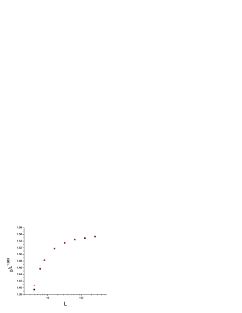
Fig. 1 shows $\chi(\beta_{c},L)/L^{2-\eta}$ against $L$ adopting $\eta=0.0368$ deng:03 ; the finite size scaling corrections in the present data can be fitted by

$$\chi(\beta_{c},L)=1.557L^{1.9632}\left(1-0.218L^{-0.82}-0.256L^{-1.65}\right)$$ (60)

The analysis is consistent with that of deng:03 ,

$$\chi(\beta_{c},L)=L^{2-\eta}\left(1.559(16)-0.37(5)L^{-0.8}\right)$$ (61)

Because of the introduction of a next to leading term, the fit extends to lower $L$.

Figure 2: (Color online) The normalized derivative of the susceptibility $[(\partial\chi(\beta,L)/\partial\beta))/\chi(\beta,L)]_{\beta_{c}}$ against $L^{1/\nu}$. The extended scaling value for the intercept is $-(2-\eta)/2\beta_{c}$ to leading order (red arrow)

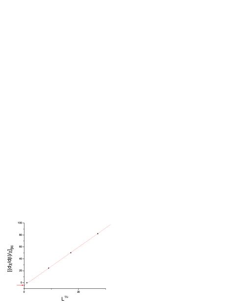
Fig. 2 shows partial data for the ratio

$$x(L)=[(\partial\chi(\beta,L)/\partial\beta)/\chi(\beta,L)]_{\beta_{c}}$$ (62)

against $L$. On this scale the data can be well represented by $x(L)=-(2-\eta)/2\beta_{c}+K_{1}L^{-1/\nu}$ with $\beta_{c}=0.2216549$, $\eta=0.0368(2)$, $\nu=0.6302(1)$, and $K_{1}$ a constant, see the extended scaling expression Eq.(53). This form of plot provides an independent estimate for $\nu$ consistent with the values given in butera:02 ; deng:03 ; lundow:10 . To obtain an accurate value for $\nu$ it is important to include the non-zero intercept.

Combining $\nu$ and $\eta$ estimates from FSS at criticality, the present data are almost consistent with the MC and HTSE estimates $\gamma=(2-\eta)\nu=1.2372(4)$ deng:03 and $\gamma=1.2371(1)$ butera:02 . Both of these are from meta-analyses on many systems in the same universality class, the latter relying principally on bcc data. A recent very precise study of the 3d Ising universality class hasenbusch:10a gave $\nu=0.63002(10)$ and $\eta=0.03627(10)$ so $\gamma=1.2372(3)$ together with $\omega=\theta/\nu=0.832(6)$ so $\theta=0.524(4)$.

Leaving the pure FSS regime, now consider the overall temperature and size dependence of $\chi(\beta,L)$. Assuming $\beta_{c}$ known, the critical exponent $\gamma_{c}$ can be estimated directly and independently from an extrapolation to $\tau=0$ of the derivative $\gamma_{\mathrm{eff}}(\tau,\infty)=\partial\log\chi(\beta,L)/\partial\log\tau$ in the thermodynamic limit conditions i.e. down to $L$-dependent crossover temperatures above which the $\chi(\beta,L)$ are independent of $L$. The crossover occurs when $L\approx 6\xi(\beta,\infty)$, below which the correlation length is no longer negligible compared to the sample size. (As $T\to T_{c}$ below this crossover, $\chi(\beta,L)$ then tends to a constant for each $L$).

There is obviously no ”critical-to-classical crossover” as a function of temperature. The crossover would appear automatically if the effective exponent were defined (e.g. Ref. luijten:97 ) in terms of the thermodynamic susceptibility

$$\chi_{\mathrm{th}}(\beta)=[\partial m(\beta,h)/\partial h]_{h\to 0}\equiv\beta\chi(\beta)$$ (63)

and the traditional scaling variable $t$ through

$$\gamma_{\mathrm{th,eff}}=\partial\log\chi_{\mathrm{th}}(\beta)/\partial\log t$$ (64)

because at high temperatures $\chi_{th}(\beta)\to\beta$ and $t\to T$.

The present data for $L=64$, $L=32$ and $L=16$ are of very high statistical accuracy. Again assuming $\beta_{c}=0.221655$, $\gamma_{\mathrm{eff}}(\tau,L)$ values in the thermodynamic limit conditions (which are in excellent agreement with HTSE data for $\gamma_{\mathrm{eff}}(\tau,\infty)$ butera:02 ; butera:priv ), can be extrapolated satisfactorily to $\tau=0$ assuming $\gamma_{\mathrm{eff}}(\tau,\infty)=\gamma_{c}+a_{1}\tau^{\theta}+\cdots$, Fig 3. The fit provides an estimate $\gamma=1.239(1)$, almost compatible with the HTSE butera:02 and FSS deng:03 estimates.

Figure 3: (Color online) An overall plot of the effective exponent $\gamma_{\mathrm{eff}}(\tau,L)$ fixing $\beta_{c}=0.221655$ and $\theta=0.50$ for sizes $L=64,32,16$ from top to bottom (black, blue, green). The thermodynamic limit envelope curve is clearly seen. The red line corresponds to an HTSE data analysis butera:02 ; butera:priv , in full agreement with the present results over the entire temperature range except for a marginal difference near $\beta_{c}$. The red arrow indicates the consensus value for $\gamma(\beta_{c})$.

Figure 4: (Color online) As Fig 3, blowup of the small $\tau$ region.

The fluctuations in the plot for $L=64$ in Fig. 4 are an indication of how sensitive these plots are to the slightest noise in the original data. The temperature region in the far right of Fig. 4 for $L=64$ corresponds to a region of energy levels measured at least 500,000 times. At the other end the energy levels were measured more than 1,000,000 times. Data for still higher $L$ are not shown as the fluctuations become more marked; unfortunately these higher $L$ data cannot be used to refine the estimate of $\gamma$. The $\gamma$ estimate with the present method is sensitive to the value assumed for $\theta$. The $\gamma$ estimate would become incompatible with the consensus value if one assumed significantly higher values for $\theta$, such as $0.54$ (estimates of $\theta$ are reviewed in butera:02 ).

An advantage of this $\gamma_{\mathrm{eff}}(\tau,\infty)$ technique is that it is free from the problem of finite size corrections to scaling, although the Wegner thermal corrections to scaling must be taken into account as above. It can be noted also that this is a direct measurement of $\gamma$ rather than an indirect estimate through a combination of $\nu_{c}$ and $2-\eta_{c}$ estimates as is the case for FSS.

Figure 5: (Color online) The normalized susceptibility $\chi(\beta,L)\tau^{\gamma}$ against $\tau^{\theta}$ assuming $\gamma=1.239$ and $\theta=0.50$. Sizes $L=256,128,64,32,16,8$ from top to bottom (black, red, green, blue, olive, orange). The excellent fit (yellow) to the thermodynamic limit envelope data corresponds to Eq.(65).

Figure 6: (Color online) The normalized correlation length $\xi(\beta,\infty)\tau^{\nu}\beta^{1/2}$ against $\tau^{\theta}$ in the thermodynamic limit assuming $\nu=0.630$ and $\theta=0.50$. Raw HTSE data provided by P. Butera butera:02 ; butera:priv .

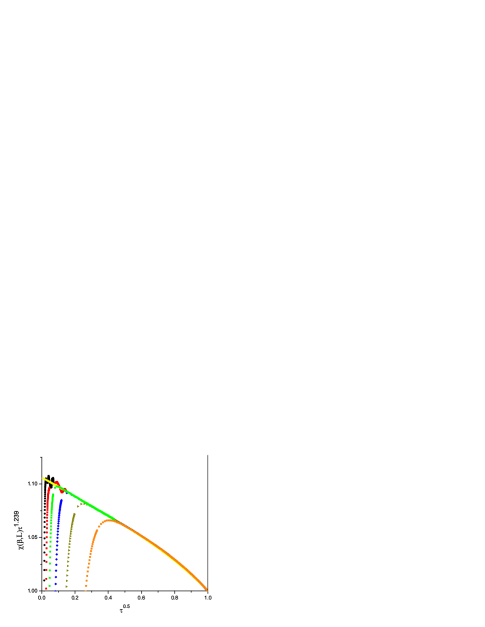
Fig. 5 shows the data for $L=16$ to $L=256$ in the form of a normalized plot, $\chi(\beta,L)\tau^{\gamma}$ against $\tau^{0.50}$ assuming $\gamma=1.239$. Again it can be seen by inspection at which point for each $L$ the curves leave the thermodynamic limit envelope curve which is $L$ independent. With the scaling expression Eq.(VI) and using the data at the various $L$ but only in the thermodynamic limit, the fit

$$\chi(\beta,\infty)\tau^{\gamma}=1.106\left(1-0.080\tau^{\theta}-0.016\tau\right)$$ (65)

gives the values of the critical amplitude, $C_{\chi}=1.106(5)$, and the coefficient of the leading conformal and analytic correction terms, $a_{\chi}=-0.080(3)$ and $b_{\chi}=-0.016(3)$, read directly off the plot in Fig. 5. These values are fully consistent with but more precise than earlier estimates from HTSE, $C_{\chi}=1.11(1)$ and $a_{\chi}=-0.10(3)$ butera:98 , see campbell:08 . It can be seen that the extended scaling expression with only two leading Wegner correction terms gives a very accurate fit to the data over the whole temperature range above the critical temperature.

If exactly the same data were expressed using $t=(T-T_{c})/T_{c}$ as the scaling variable rather than $\tau$, because $\tau=t/(1+t)$ one would have to write

$$\chi(\beta,\infty)=~{}~{}~{}~{}~{}~{}~{}~{}~{}~{}~{}~{}~{}~{}$$ (66)

$$1.106t^{-1.239}(1+1.239t+0.1466t^{2}-0.0373t^{3}+\cdots$$

$$-0.080t^{0.5}+0.0495t^{1.5}-0.0371t^{2.5}+\cdots$$

$$-0.016t+0.016t^{2}-0.016t^{3}+\cdots)$$

Remembering that $t$ diverges at infinite $T$, each of the correction terms in the sums is individually diverging at high temperatures. Manifestly it is considerably more efficient to scale $\chi(\beta,\infty)$ with $\tau$ rather than with $t$.

We have made no correlation length measurements. However we have carried out an extended scaling parametrization of HTSE thermodynamic limit second moment correlation length $\xi(\beta,\infty)$ data supplied by P. Butera butera:02 ; butera:priv .

Figure 7: (Color online) The extended scaling effective exponent $\nu(\tau)$ against $\tau^{\theta}$ in the thermodynamic limit assuming and $\theta=0.50$. Raw HTSE data provided by P. Butera butera:02 ; butera:priv

Fig. 6 shows a plot of the normalized correlation length $\xi(\beta,\infty)\tau^{\nu}\beta^{1/2}$ against $\tau^{\theta}$ assuming $\nu=0.630$ and $\theta=0.50$. The data can be fitted well by the extended scaling Wegner expression with two leading terms only

$$\xi(\beta,\infty)\tau^{\nu}\beta^{1/2}=1.074\beta^{-1/2}\left(1-0.120\tau^{0.5}+0.051\tau\right)$$ (67)

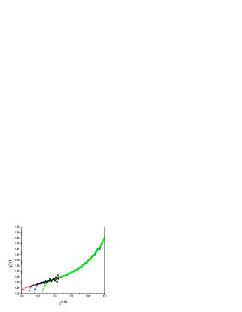
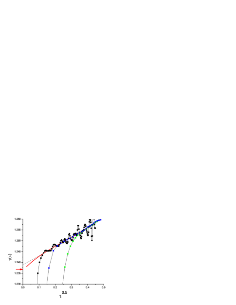
(note that here the critical amplitude is $C_{\xi}/\beta_{c}^{1/2}$). The same equation provides the temperature dependence of the effective exponent defined by

$$\nu_{\mathrm{eff}}(\beta,\infty)=\partial\log(\xi(\beta,\infty)/\beta^{1/2})/\partial\log\tau$$ (68)

see Fig. 7. The effective exponent varies only by a few percent over the whole range from $T=T_{c}$ to $T=\infty$. It is clear that the $\beta^{1/2}$ prefactor is an essential part of the temperature dependence of the correlation length. The compact relation Eq.(67) is very useful as it allows finite size scaling analyses of the entire data set for $\chi(\beta,L)$.

IX Finite size scaling

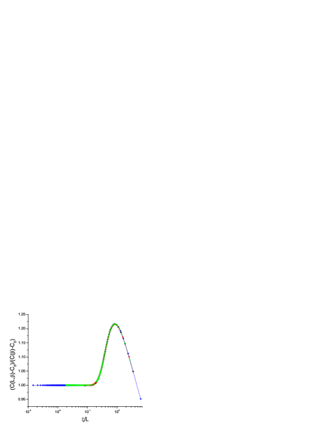
The extrapolation in Fig. 5 concerns only data in the thermodynamic limit condition for each $L$. With Eq.(67) in hand we can plot all the data and not just the points in the thermodynamic limit condition by appealing to the Privman-Fisher relation privman:84 , Eq.(II).

As a first step we ignore corrections to scaling and draw, Fig. 8, the leading order extended scaling FSS campbell:06 plot for the susceptibility

$$\chi(L,T)/(LT^{1/2})^{2-\eta}=F_{\chi}\left((LT^{1/2})^{1/\nu}\tau\right)$$ (69)

On the scale of the plot the scaling is already reasonable for all $T$ above $T_{c}$.

Figure 8: (Color online) The leading order extended scaling plot $\chi(L,T)/(L(T/T_{c})^{1/2})^{2-\eta}$ against $\left((LT^{1/2})^{1/\nu}\tau\right)$

The conformal correction can then be introduced :

$$\chi(\beta,L)/\chi(\beta,\infty)$$ (70)

$$=F_{\chi}\left(L/\xi(\beta,\infty)\right)(1+a_{\chi}L^{-\omega}G_{\chi}\left(L/\xi(\beta,\infty)\right))$$

The function $F(x)$ must have limits $F(x)\to 1$ at large $x$ and $F(x)\sim x^{2-\eta}$ for small $x$. An explicit compact ansatz which gives these limits automatically is

$$F_{\chi}(x)=\left((1-\exp(-bx^{(2-\eta)/a})\right)^{a}$$ (71)

where $x=L/\xi(\beta,\infty)$. In the critical limit $x\ll 1$,

$$F_{\chi}(x)=b^{a}(L/\xi(\beta,\infty))^{2-\eta}.$$ (72)

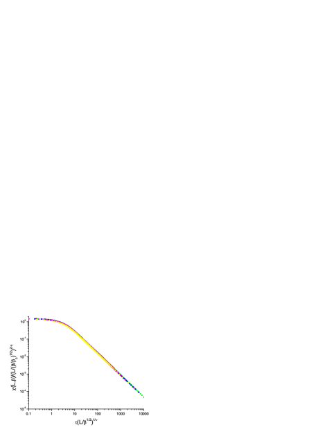
By convention $G_{\chi}\left(0\right)=1$. Fig. 9 uses the temperature dependence of the thermodynamic limit correlation length, Eq.(67), and the thermodynamic limit susceptibility, Eq.(65), to scale the data for all $L$ and all $\beta$ using Eq.(IX) for $\chi(\beta,L)$.

Figure 9: (Color online) The Privman-Fisher scaling plot $\chi(\beta,L)/\chi(\beta,\infty)$ against $L/\xi(\beta,\infty)$. $L=256,128,64,32,16$, (black, red, green, blue,cyan)

Figure 10: (Color online)The leading correction scaling function $G(L/\xi(\beta,\infty))$. Black squares: measured; red circles: fit

The principle scaling function $F(x)$ and the leading correction scaling function $G(x)$ were extracted from the data. With the numerical constant $2-\eta$ fixed at $1.963$, an accurate effective functional form for the principal scaling function is

$$F_{\chi}(x)=[1-\exp(-0.4179x^{1.963/1.262})]^{1.262}$$ (73)

On the scale of the figure $F(x)$ with these fit values ($a=1.262,b=0.4179$) is indistinguishable from the overall curve in Fig. 9. By comparing data at small $L$ with data at large $L$ the correction to scaling function can also be estimated. A fit gives $a_{\chi}\approx-0.22$ and

$$G_{\chi}(x)\approx\exp\left(-0.038x^{2.5}\right)$$ (74)

Fig. 10 shows the correction scaling function $G(x)$ together with the ad hoc Gaussian fit.

These FSS functions are universal to within metric constants fisher:72 .

In the same critical limit, from the definitions above $\chi(\beta,\infty)=C_{\chi}\tau^{-\gamma}$ and $\xi(\beta,\infty)=C_{\xi}\tau^{-\nu}$ so with $\chi(\beta_{c},L)=C^{{}^{\prime}}_{\chi}L^{2-\eta}$ in the large $L$ limit,

$$b^{a}=C^{{}^{\prime}}_{\chi}C_{\xi}^{2-\eta}/C_{\chi}$$ (75)

The amplitudes $C^{{}^{\prime}}_{\chi},C_{\chi}$ and $C_{\xi}$ are known from critical and thermodynamic limit measurements respectively, so the scaling form Eq.(72) has in principle only one free parameter, $a$. Remarkably, when the other parameters are known, the FSS crossover function can be encapsulated in one single parameter.

The overall scaling function expression covers all $L$ and all $T$ above $T_{c}$. The principle scaling function Eq.(71) contains only one free parameter; it resembles the finite size scaling form which has been used for the $2$d Villain model katzgraber:08 . Previous expressions for principle finite scaling functions caracciolo:95 ; kim:96 , in particular for the $3$d Ising model kim:96 , were in the form of infinite series in $\exp(-x)$ and so contained many fit parameters.

It would be of interest to study other members of the same family of models in order to see if the compact form of scaling function Eq.(71) is generally valid, and how the universality is expressed in the parameters $a$ and $b$.

Even below $T_{c}$ it has been noted that there should be a relationship between the non-connected reduced susceptibility and the non-connected correlation length hukushima:09 . The extended scaling gives explicit leading order predictions for the asymptotic relations both above and below $T_{c}$ between the finite size non-connected reduced susceptibility $\chi(\beta,L)$ and the finite size non-connected correlation length $\xi(\beta,L)$. As we have seen, in the limit $\xi(\beta,L)/L\ll 1$

$$\chi(\beta,L)/(LT^{1/2})^{2-\eta}\sim(\xi(\beta,L)/L)^{2-\eta}$$ (76)

while in the opposite limit $\xi(\beta,L)/L\gg 1$ the predicted relation is

$$\chi(\beta,L)/(LT^{1/2})^{2-\eta}\sim(\xi(\beta,L)/L)^{(2/d)(d-2+\eta)}$$ (77)

For the case of the $2$d square lattice Ising model the data confirm both these relationships campbell:06 ; hukushima:09 . Unfortunately, as we have no data here for the finite size $\xi(\beta,L)$ either above or below $T_{c}$ we cannot check the relationship.

X Susceptibility above and below $T_{c}$

The ratios of susceptibility amplitudes and of leading correction factors above and below $T_{c}$ are universal. The standard reduced susceptibility for the region above $T_{c}$ has been discussed; for $T$ above and below $T_{c}$ we will plot the modulus susceptibility Eq.(6) multiplied by $|\tau|^{\gamma}$ as a function of $|\tau|^{\theta}$ with exponent values fixed at $\gamma=1.239,\theta=0.50$, Fig. 11.

Figure 11: (Color online) The normalized modulus susceptibility $\chi_{\mathrm{mod}}(\tau)|\tau|^{\gamma}$ as a function of $|\tau|^{\theta}$. The upper set of curves corresponds to $T>T_{c}$ and the lower set to $T<T_{c}$. In both cases the sizes are $L=64,32,16$ (black, red, blue).

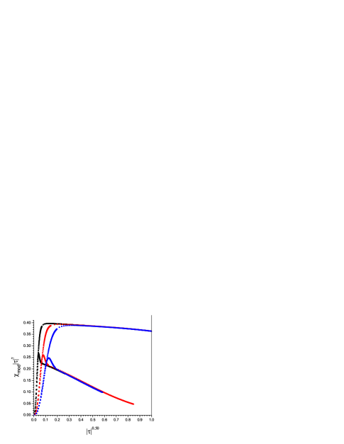
By definition $\chi_{\mathrm{mod}}$ becomes equal to the connected reduced susceptibility below $T_{c}$ in the thermodynamic large $L$ limit. Extrapolating the data corresponding to this limit to $|\tau|=0$ we find to leading order

$$\chi_{\mathrm{conn}}=C_{\chi,-}|\tau|^{-1.239}\left(1+a_{\chi,-}|\tau|^{0.50}+\cdots\right)$$ (78)

with $C_{\chi,-}=0.241(2)$ and $a_{\chi,-}=-0.82(5)$. Taking into account the normalization factor for $\chi_{\mathrm{mod}}$, the present estimates for the amplitude ratio and the correction amplitude ratio are $C_{\chi,+}/C_{\chi,-}=4.67(3)$ and $a_{\chi,+}/a_{\chi,-}=0.111(10)$. The amplitude ratio is consistent with previous Monte-Carlo estimates, $4.75(3),4.72(11)$ and $4.713(7)$, caselle:97 ; engels:99 ; hasenbusch:10 . The present correction amplitude ratio estimate is however significantly lower than a field theory value $0.315(13)$ bagnuls:87 ; privman:91 .

XI Specific heat above and below $T_{c}$

The specific heat is intrinsically difficult to analyze because of the strong regular term $C_{0}$ and the small value of the critical exponent $\alpha$ (see Eq.(25)). It turns out in addition that there are strong and peculiar finite size corrections. On the other hand the statistical precision of the specific heat data is very high; data for $L=512$ were included in this analysis. The general leading form of the envelope data in the thermodynamic limit condition is assumed to be $\left(C_{v}(\beta,L)-C_{0}\right)|\tau_{2}|^{\alpha}=C_{c}\left(1+a_{c}|\tau_{2}|^{\theta}\right)$ where $\tau_{2}=1-(\beta/\beta_{c})^{2}$. The amplitudes are $C_{c,+},C_{c,-}$ and $a_{c,+},a_{c,-}$ above and below $T_{c}$ respectively. Here $\alpha$ is fixed at $0.110$, which is the expected value from the relation $\alpha=\nu d-2$ with $\nu=0.630$. The regular term $C_{0}$ is assumed to be temperature independent; the estimate $C_{0}=-30.9$ is obtained from the overall fit discussed below. It should be underlined that the extended scaling variable is $\tau_{2}$ not $\tau$.

In the high temperature range (down to $\beta\approx 0.2$) the data can be compared to data points derived by directly summing the HTSE terms up to $n=46$ from Ref. arisue:03 . Point by point agreement is better than to $1$ part in $10^{3}$.

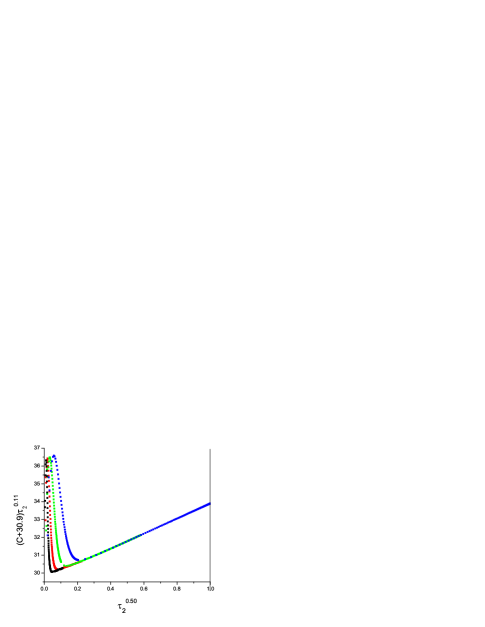
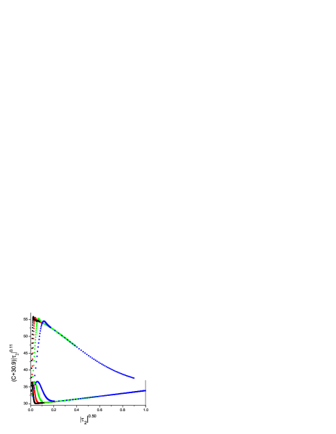
As a first step we plot the raw $\log C_{v}(\tau_{2},L)$ above $T_{c}$ against $\log\tau_{2}$, Fig. 12. The thermodynamic limit data for different $L$ can be clearly observed but the points fall on a curve rather on a straight line even down to very small $\tau_{2}$; this is because no $C_{0}$ term has been allowed for. Next, we plot $\log\left(C_{v}(\tau_{2},L)-C_{0}\right)$ against $\log\tau_{2}$, as in Fig. 13 for various trial values of $C_{0}$. In Fig. 13 with $C_{0}=-30.9$ the envelope data now lie on a straight line of slope $-0.110$ for the lower range of $\tau_{2}$ (and the larger $L$). We make a Privman-Fisher finite size scaling plot of $\left(C_{v}(\tau_{2},L)+30.9\right)/\left(C_{v}(\tau_{2},\infty)+30.9\right)$ against $L/\xi(\tau_{2},\infty)$ with $\left(C_{v}(\tau_{2},\infty)+30.9\right)$ taken from the extrapolated envelope for small $\tau_{2}$ and the measured envelope curve for higher $\tau_{2}$, fitted to an explicit function for $\left(C_{v}(\tau_{2},\infty)+30.9\right)$, Fig. 14. The thermodynamic limit correlation length is taken from Eq.(67).

In the finite size limited $L<\xi(\tau_{2},\infty)$ region the normalized specific heat shows a strong peak, in contrast to the regular FSS crossover observed for the susceptibility. The quality of the global fit is sensitive to the value chosen for the regular term $C_{0}$ as the correct choice for this parameter is essential to obtain an $L$-independent peak height in Fig. 13. Once $C_{0}$ is fixed fine adjustments are made to the correction terms so as to obtain an $L$- and $T$-independent flat plateau in the left hand side thermodynamic limit region.

An excellent global Eq.(II) FSS fit is obtained taking

$$C_{v}(\tau_{2},\infty)=~{}~{}~{}~{}~{}~{}~{}~{}~{}~{}~{}~{}~{}~{}~{}~{}~{}~{}~{}~{}~{}~{}~{}~{}~{}$$ (79)

$$-30.9+29.85\tau_{2}^{-0.11}\left(1+0.12\tau_{2}^{0.5}+0.014\tau_{2}\right)$$

The optimal value $C_{0}=-30.9(5)$ can be compared with previous estimates : $-33.3(24)$ hasenbusch:98 and $-27.85(80)$ feng:10 .

The normalized $(C_{v}(\tau_{2},\infty)+30.9)\tau_{2}^{0.11}$ is shown in Fig. 15 where the nearly linear thermodynamic limit envelope is obvious.

Figure 12: (Color online) Raw $\log C_{v}(\beta,L)$ against $\log\tau_{2}=\log(1-(\beta/\beta_{c})^{2})$. The sizes are from left to right $L=512,256,128,64,32$, (black, red, green, blue, cyan)

Figure 13: (Color online) $\log(C_{v}(\beta,L)+30.9)$ against $\log\tau_{2}$. The sizes are from left to right $L=512,256,128,64,32,16$, (black, red, green, blue, cyan, magenta). The dashed line has the slope $-0.110$.

Figure 14: (Color online) The specific heat finite size scaling fit. The ratio $\left(C_{v}(\beta,L)-C_{0}\right)/\left(C_{v}(\beta,\infty)-C_{0}\right)$ against $\xi(\beta,\infty)/L$ with $C_{0}=-30.9$. Sizes are $L=512,256,128,64$, (black, red, green, blue)

Figure 15: (Color online) $\left(C_{v}(\beta,L)-C_{0}\right)\tau_{2}^{\alpha}$ against $\tau_{2}=1-(\beta/\beta_{c})^{2}$ with $\alpha=0.110$ and $C_{0}=-30.9$ for all temperatures $T>T_{c}$. Sizes $L=256,128,64,32$, (black, red, green, blue).

Figure 16: (Color online) $\left(C_{v}(\beta,L)-C_{0}\right)|\tau_{2}|^{\alpha}$ against $|\tau_{2}|=|1-(\beta/\beta_{c})^{2}|$ with $\alpha=0.110$ and $C_{0}=-30.9$. The lower set of curves corresponds to $T>T_{c}$ and the upper set to $T<T_{c}$. Sizes $L=256,128,64,32$, (black, red, green, blue).

The $C_{v}(\beta,\infty)$ from Eq.(XI) together with the peaked FSS curve (for which we have no explicit algebraic expression) provide an accurate representation of the specific heat at all temperatures above $T_{c}$ and for all sizes $L$. This is in contrast to previous analyses of MC data which were made in terms of truncated series of terms.

The ratios of critical amplitudes and of leading correction amplitudes above and below $T_{c}$ are universal. The data show critical amplitudes $C_{c,+}=29.9(1)$ and $C_{c,-}=55.4(2)$ above and below $T_{c}$, Fig. 16. With the extended scaling definition, $C_{c,+}=A_{c}2^{\alpha}/\beta_{c}^{2}$ where $A_{c}$ is the amplitude using the standard definition. The present $C_{c,+}$ result is in very good agreement with the HTSE estimate $A_{c}=1.34(1)$ given in Ref. butera:02 which corresponds to $C_{c,+}=29.4(3)$. The present estimate for the amplitude ratio (which is definition independent) is $C_{c,+}/C_{c,-}=0.540(4)$, consistent with $\epsilon$-expansion and field theory values of $0.524(10)$ and $0.541(14)$ respectively privman:91 , and with the most recent MC values $0.532(7)$ and $0.536(2)$ feng:10 ; hasenbusch:10 . For the correction amplitudes the data indicate (Fig. 15 and 16) $a_{c,+}\approx 0.12$ and $a_{c,-}\approx-0.23$, so $a_{c,+}/a_{c,-}\approx-0.52$ and $a_{c,+}/a_{\chi,+}\approx 1.4$. These values can be compared with field theory estimates, $0.96(25)$ and $0.95(10)$ respectively bagnuls:81 ; bagnuls:87 ; privman:91 . (It should be noted that the $a_{c}$ values in our notation correspond to $a_{c}\alpha$ in the notation of Refs.  bagnuls:81 ; bagnuls:87 .)

We cannot carry out a full FSS analysis below $T_{c}$ as we lack information on the correlation length.

XII Conclusion

We have applied the extended scaling approach to the analysis of two canonical Ising ferromagnet models : the historic $S=1/2$ ferromagnet on a $1$d chain, and the $S=1/2$ ferromagnet on the simple cubic lattice.

For the $1$d model, with the scaling variables $\tau=(1-\tanh\beta)$ for the susceptibility and the correlation length and $\tau_{2}=(1-\tanh\beta)^{2}$, all the analytic thermodynamic limit expressions are of precisely the extended scaling form over the entire temperature range from zero to infinity, with no confluent corrections, Eqns. 34, 35, 36.

An appropriate scaling variable for reduced susceptibility and second moment correlation length in a ferromagnetic Ising model with a non-zero ordering temperature is $\tau=1-\beta/\beta_{c}=(T-T_{c})/T$, not the traditional $t=(T-T_{c})/T_{c}$. An exhaustive analysis of high quality numerical data for the $3$d Ising model demonstrates that the reduced susceptibility and the second moment correlation length can be represented satisfactorily over the entire temperature range above $T_{c}$ by compact expressions containing two leading Wegner correction terms only :

$$\chi(\beta,\infty)=1.106\tau^{-1.239}\left(1-0.080\tau^{0.5}-0.016\tau\right)$$ (80)

and

$$\xi(\beta,\infty)=1.074\beta^{1/2}\tau^{-0.630}\left(1-0.109\tau^{0.5}+0.039\tau\right)$$ (81)

For the specific heat on a bipartite lattice (such as the sc lattice) the appropriate extended scaling variable is $\tau_{2}=1-(\beta/\beta_{c})^{2}$. The data from $T_{c}$ to infinite temperature can be fitted accurately by

$$C_{v}(\beta,\infty)=~{}~{}~{}~{}~{}~{}~{}~{}~{}~{}~{}~{}~{}~{}~{}~{}~{}~{}~{}~{}~{}~{}~{}~{}~{}~{}~{}~{}~{}~{}~{}$$ (82)

$$-30.9+29.85\tau_{2}^{-0.110}\left(1+0.12\tau_{2}^{0.5}+0.014\tau_{2}\right)$$

We give explicit finite size susceptibility scaling functions for the two models. The principle $1$d susceptibility scaling function

$$\chi(\beta,L)/\chi(\beta,\infty)=\tanh(L/2\xi(\beta,\infty))$$ (83)

is exact. The principle $3$d susceptibility scaling ansatz

$$\chi(\beta,L)/\chi(\beta,\infty)=[1-\exp(-b(L/\xi(\beta,\infty))^{(2-\eta)/a})]^{a}$$ (84)

with $a=1.262$, $b=0.4179$ fits the data to high precision. This form where two parameters encapsulate the finite size scaling crossover from the region $L\gg\xi(\beta,\infty)$ to the region $L\ll\xi(\beta,\infty)$ might well be of generic application.

The critical parameters can be estimated by combining the data in the thermodynamic limit $L\gg\xi_{\infty}(\beta)$ with the data in the finite size scaling region $L\ll\xi_{\infty}(\beta)$. The results provide complementary estimates for critical amplitudes and critical amplitude ratios.

The aim of this work is however not so much to improve on the already very accurate existing estimates for universal critical parameters in the intensively studied ferromagnetic $3$d Ising model, but to explain the rationale leading to an optimized choice of scaling variables and scaling expressions for covering the whole temperature range up to infinite temperature. Here we spell out in detail for two canonical examples, the $1$d and $3$d Ising ferromagnets, an ”extended scaling” methodology for studying numerical data taken over the entire temperature range without restricting the analysis to a narrow ”critical” temperature region near $T_{c}$. Scaling variables and scaling expressions are chosen following a simple unambiguous prescription inspired by the well established HTSE approach. Using these and allowing for small leading Wegner correction terms where necessary, critical scaling expressions for $\chi(\beta,\infty)$, $\xi(\beta,\infty)$ and $C_{v}(\beta,\infty)$ remain valid to high precision from $T_{c}$ right up to infinite temperature. Residual analytic correction terms are either strictly zero (in $1$d) or very weak (in $3$d).

The approach can readily be generalized to other less well understood systems.

XIII Appendix A : General spin S

Standard expressions for the reduced susceptibility and the correlation length for ferromagnets as defined in butera:02 are for general spin $S$

$$\chi(\tau)=C_{\chi}^{S}(std)\tau^{-\gamma}\left(1+F_{\chi}(\tau)\right)$$ (85)

and

$$\xi(\tau)=C_{\xi}^{S}(std)\tau^{-\nu}\left(1+F_{\xi}(\tau)\right)$$ (86)

The extended scaling prescription consists in transposing each HTSE expression such that it takes the form of a series in a variable $x$, having leading term $1$ and multiplied by a prefactor. In the case of a finite critical temperature Ising ferromagnet with $\tau=1-\beta/\beta_{c}$, the critical amplitudes are then defined through

$$\chi(\beta,\infty)=C_{\chi}(es)\tau^{-\gamma}\left(1+F_{\chi}(\tau)\right)$$ (87)

(c.f. Eq.(1)) and

$$\xi(\beta,\infty)=C_{\xi}(es)\beta^{1/2}\tau^{-\nu}\left(1+F_{\xi}(\tau)\right)$$ (88)

For general Ising spin $S$, dimension $d$, and a lattice with $z$ nearest neighbors the extended scaling critical amplitudes are

$$C_{\chi}^{S}(es)=\left((S+1)/3S\right)C_{\chi}^{S}(std)$$ (89)

and

$$C_{\xi}^{S}(es)=C_{\xi}^{S}(std)/\left(z(1+S)\beta_{c}/6dS\right)^{1/2}$$ (90)

The definitions of the effective exponents are unaltered.

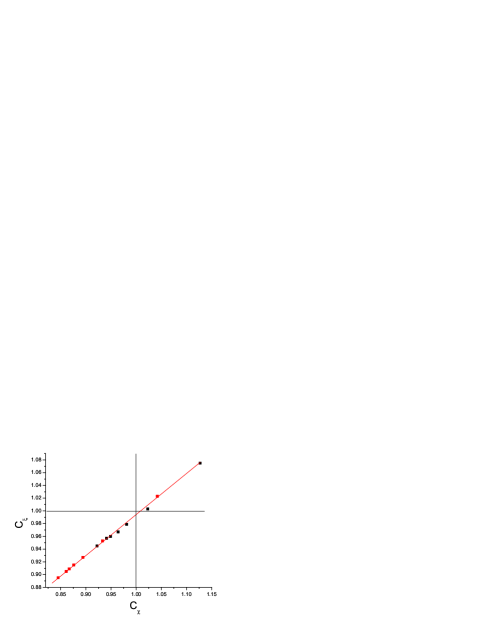
With these normalizations the physical significance of the critical amplitudes becomes much more transparent. Ref. butera:02 lists the standard critical amplitudes as functions of $S$ for sc and bcc lattices. In Table AI we compare these values with those obtained using the above definitions. The extended scaling values are close to $1$ for all $S$; the differences $\left(C_{Q}^{S}(es)-1\right)$ which can be read directly from the Table are a quantitative indication, model by model, of the amplitude of the $S$-dependent correction terms within $F_{Q}^{S}$.

Table 1: Values of the critical amplitudes for spin $S$ with the standard definitions, Eqns. 85 and 86 Ref. butera:02 compared with values using the extended scaling definitions Eqns. 89 and 90

$S$	$1/2$	$1$	$3/2$	$2$	$5/2$	$3$	$\infty$
$sc$
$C_{\chi}(std)$	$1.127$	$0.682$	$0.545$	$0.482$	$0.443$	$0.418$	$0.307$
$C_{\xi}(std)$	$0.506$	$0.458$	$0.443$	$0.436$	$0.432$	$0.430$	$0.423$
$C_{\chi}(es)$	$1.127$	$1.023$	$0.981$	$0.964$	$0.949$	$0.941$	$0.922$
$C_{\xi}(es)$	$1.075$	$1.003$	$0.979$	$0.967$	$0.960$	$0.957$	$0.945$
$bcc$
$C_{\chi}(std)$	$1.042$	$0.622$	$0.497$	$0.438$	$0.404$	$0.383$	$0.282$
$C_{\xi}(std)$	$0.469$	$0.426$	$0.411$	$0.405$	$0.401$	$0.399$	$0.394$
$C_{\chi}(es)$	$1.042$	$0.933$	$0.894$	$0.876$	$0.867$	$0.861$	$0.845$
$C_{\xi}(es)$	$1.023$	$0.953$	$0.927$	$0.915$	$0.909$	$0.905$	$0.895$

If the corrections to scaling up to infinite temperature are dominated by the leading (confluent) term then $C_{\chi}^{S}(es)-1\approx a_{\chi}(S)$ and $C_{\xi}^{S}(es)-1\approx a_{\xi}(S)$. The universal ratio $a_{\xi}(S)/a_{\chi}(S)\approx(C_{\xi}^{S}(es)-1)/(C_{\chi}^{S}(es)-1)$. From Fig. 13 which shows the data from the Table, we can estimate $a_{\xi}(S)/a_{\chi}(S)\approx 0.65(2)$ (with a small offset corresponding to the next-to-leading correction). This compares favorably with the estimates $0.76(6)$ from HTSE butera:02 , $0.65(5)$ obtained by the RG in the perturbative fixed-dimension approach at sixth order bagnuls:86 , and $0.65$ from the $\epsilon$ expansion to second order chang:83 .

Figure 17: (Color online) $C_{\xi}^{S}(es)$ plotted against $C_{\chi}^{S}(es)$, where $C_{\xi}^{S}(es)$ and $C_{\chi}^{S}(es)$ are spin $S$ dependent extended scaling susceptibility and correlation length critical amplitudes. Black points sc lattice, red points bcc lattice. See text, Ref. butera:02 , and Table AI.

XIV Appendix B: Ising spin glass

It can be noted that in the case of the Ising Spin Glass the energy scale of the interactions is fixed by $\langle J_{ij}^{2}\rangle$ not by $\langle J\rangle$ as in the ferromagnetic case ($\langle J_{ij}\rangle$ is zero in a symmetric interaction distribution spin glass). From an obvious dimensional argument the normalized spin glass ”temperature” should be $T^{2}/\langle J_{ij}^{2}\rangle$. It has long been recognized that for the spin glass the HTSE expressions contain even terms only (i.e. an expansion in $(\beta/\beta_{c})^{2}$ or $(\tanh\beta/\tanh\beta_{c})^{2}$ rather than in $\beta/\beta_{c}$) so the appropriate scaling variable is $\tau_{sg}=1-(\beta/\beta_{c})^{2}$ or $1-(\tanh\beta/\tanh\beta_{c})^{2}$ fisch:77 ; singh:86 ; klein:91 ; daboul:04 . The argument presented above for the ferromagnet can be repeated mutatis mutandis on this basis; the extended scaling expressions for $\chi(\beta,L)$ and $\xi(\beta,L)$ in spin glasses are the same as those for the ferromagnet (Eqns. 17 and  18) but with $(\beta/\beta_{c})^{2}$ substituted for $\beta/\beta_{c}$ everywhere campbell:06 .

Unfortunately the great majority of publications on spin glasses have used $t$ as the scaling variable which is quite inappropriate except for a very restricted range of temperatures near $T_{c}$. One consequence is that many published estimates of the exponent $\nu$ in spin glasses are low by a factor of about $2$ (see the discussion in katzgraber:06 ).

XV Acknowledgements

We would like to thank Paolo Butera for generously providing us with tabulated data sets and for helpful comments. We thank V. Privman for an encouraging comment. This research was conducted using the resources of High Performance Computing Center North (HPC2N).

99

References

- (1) F. J. Wegner, Phys. Rev. B 5, 4529 (1972).
- (2) V. Privman, P.C. Hohenberg and A. Aharony, in Phase Transitions and Critical Phenomena, edited by C. Domb and J.L. Lebowitz , Vol. 14 (Academic Press, New York, 1991).
- (3) A. Pelissetto and E. Vicari, Phys. Rep. 368, 549 (2002).
- (4) E. Luijten, H. W. J. Blöte, and K. Binder, Phys. Rev. Lett. 79, 561 (1997).
- (5) Y. Garrabos and C. Bervillier, Phys. Rev. E 74, 021113 (2006).
- (6) M. Fähnle and J. Souletie, J. Phys. C 17 L469 (1984).
- (7) S. Gartenhaus and W. S. McCullough, Phys. Rev. B 38, 11688 (1988).
- (8) J.-K. Kim, A. J. F. de Souza and D. P. Landau, Phys. Rev. E 54, 2291 (1996).
- (9) P.Butera and M. Comi, Phys. Rev. B, 65 144431 (2002).
- (10) Y. Deng and H. W. J. Blöte, Phys. Rev. E 68, 036125 (2003).
- (11) M. Caselle, M. Hasenbusch, J. Phys. A 30, 4963 (1997) [hep-lat/9701007].4.75(3).
- (12) I. A. Campbell, K. Hukushima, and H. Takayama, Phys. Rev. Lett. 97, 117202 (2006).
- (13) I. A. Campbell, K. Hukushima, and H. Takayama, Phys. Rev. B 76, 134421 (2007).
- (14) H. G. Katzgraber, I. A. Campbell and A. K. Hartmann, Phys. Rev. B 78, 184409 (2008).
- (15) I. A. Campbell and P. Butera, Phys. Rev. B 78 024435, (2008).
- (16) K. Hukushima, I.A. Campbell and H. Takayama, Int. J. Mod. Phys. C 20, 1 (2009).
- (17) R. Häggkvist, A. Rosengren, D. Andrén, P. Kundrotas, P. H. Lundow and K. Markström, J. Stat. Phys. 114 455 (2004).
- (18) R. Häggkvist, A. Rosengren, P. H. Lundow, K. Markström, D. Andrén and P. Kundrotas, Adv. Phys. 56 653 (2007).
- (19) M. E. Fisher and R. J. Burford, Phys. Rev. 156, 583 (1967).
- (20) E. Brézin, J. Phys. (Paris) 43 15 (1982).
- (21) P. Calabrese, V. Martin-Mayor, A. Pelissetto, and E. Vicari, Phys. Rev. E 68, 036136 (2003).
- (22) J. G. Darboux, J. Math. Pures Appl. 4, 377 (1878).
- (23) P. Butera and M. Comi, arXiv:hep-lat/0204007.
- (24) F. J. Wegner, in Phase Transitions and Critical Phenomena, vol 6, ed C Domb and M S Green (New York: Academic Press) (1976).
- (25) J. Kouvel and M. E. Fisher, Phys. Rev. A 136, 1626 (1964).
- (26) G. Orkoulas, A. Z. Panagiotopoulos, and M. E. Fisher, Phys. Rev. E 61, 5930 (2000).
- (27) E. Ising, Z. der Physik 31, 253 (1925).
- (28) R. J. Baxter, Exactly solved models in statistical mechanics, Academic Press (1982).
- (29) G. A. Baker and J. C. Bonner, Phys. Rev. B 12, 3741 (1975).
- (30) B. Berche, C. Chatelain, C. Dhall, R. Kenna, R. Low, and J. -C. Walter, J. Stat. Mech. P11010 (2008).
- (31) M. Hasenbusch, A. Pelissetto, and E. Vicari, Phys. Rev. B 78, 214205 (2008).
- (32) H. G. Katzgraber, M. Körner and A. P. Young, Phys. Rev. B 73, 224432 (2006).
- (33) F. Wang and D. P. Landau, Phys. Rev. Lett. 86 2050 (2001).
- (34) J. -S. Wang and R. H. Swendsen, J. Stat. Phys. 106 245 (2002).
- (35) P. H. Lundow and K. Markström, Cent. Eur. J. Phys. 7 490 (2009).
- (36) K. Binder, Z. Phys. B: Condens. Matter 43, 119 (1981).
- (37) H. Arisue and K. Tabata, Nucl. Phys. B 435, 555 (1995).
- (38) P. H. Lundow and I. A. Campbell, Phys. Rev. B 82, 024414 (2010).
- (39) M. Hasenbusch, Phys. Rev. B 82, 174433 (2010).
- (40) J. Salas and A. D. Sokal, J. Stat. Phys. 98,551 (2000).
- (41) R. Guida and J. Zinn-Justin, J. Phys. A: Math. Gen. 31, 8103 (1998).
- (42) K. E. Newman and E. K. Riedel, Phys. Rev. B 30, 6615 (1984).
- (43) P. Butera, private communication.
- (44) P. Butera and M. Comi, Phys. Rev. B 58, 11 552 (1998).
- (45) V. Privman and M. E. Fisher, Phys. Rev. B 30 322 (1984).
- (46) M. E. Fisher, in Critical Phenomena, Proceedings of the 51st Enrico Fermi Summer School, edited by M.S. Green (Academic Press, New York, 1972).
- (47) S. Caracciolo, R. G. Edwards, S. J. Ferreira, A. Pelissetto, and A. D. Sokal, Phys. Rev. Lett. 74, 2969 (1995).
- (48) J. Engels, T. Scheideler, Nucl. Phys. B 539, 557 (1999).
- (49) M. Hasenbusch, Phys. Rev. B 82, 174433 (2010).
- (50) C. Bagnuls and C. Bervillier, Phys. Rev. B 24 1226 (1981).
- (51) C. Bagnuls, C. Bervillier, D. I. Meiron and B. G. Nickel, Phys. Rev. B 35 3585 (1987).
- (52) H. Arisue and T. Fujiwara, Phys. Rev. E 67, 066109 (2003).
- (53) M. Hasenbusch and K. Pinn, J. Phys. A 31, 6157 (1998).
- (54) X. Feng and H. W. J. Blöte, Phys. Rev. E 81, 031103 (2010).
- (55) C. Bagnuls and C. Bervillier, J. Phys. A 19, L85 (1986).
- (56) M. C. Chang and J. J. Rehr, J. Phys. A 16, 3899 (1983).
- (57) R. Fisch and A. B. Harris, Phys. Rev. Lett. 38,785 (1977).
- (58) R. R. P. Singh and S. Chakravarty, Phys. Rev. Lett. 57, 245(1986).
- (59) L. Klein, J. Adler, A. Aharony, A. B. Harris and Y. Meir, Phys. Rev. B 43 11249 (1991).
- (60) D. Daboul, I. Chang, and A. Aharony, Eur. Phys. J. B 41, 231 (2004).