On a small-gain approach to distributed event-triggered control

Abstract

In this paper the problem of stabilizing large-scale systems by distributed controllers, where the controllers exchange information via a shared limited communication medium is addressed. Event-triggered sampling schemes are proposed, where each system decides when to transmit new information across the network based on the crossing of some error thresholds. Stability of the interconnected large-scale system is inferred by applying a generalized small-gain theorem. Two variations of the event-triggered controllers which prevent the occurrence of the Zeno phenomenon are also discussed.

1 Introduction

We consider large-scale systems stabilized by distributed controllers, which communicate over a limited shared medium. In this context it is of interest to reduce the communication load. An approach in this direction is event-triggered sampling, which attempts to send data only at “relevant times”. In order to treat the large-scale case, input-to-state stability (ISS) small-gain results in the presence of event-triggering decentralized controllers are presented.
The stability (or stabilization) of large-scale interconnected systems is an important problem which has attracted much interest. In this context the small-gain theorem was extended to the interconnection of several ${\cal L}_{p}$-stable subsystems. Early accounts of this approach are [28] (see also [22]) and references therein. For instance, in [28], Theorem 6.12, the influence of each subsystem on the others is measured via an ${\cal L}_{p}$-gain, $p\in[1,\infty]$ and the ${\cal L}_{p}$-stability of the interconnected system holds provided that the spectral radius of the matrix of the gains is strictly less than unity. In other words, the stability of interconnected ${\cal L}_{p}$-stable systems holds under a condition of weak coupling.
In the nonlinear case a notion of robustness with respect to exogenous inputs is input-to-state stability (ISS) ([23]). If in a large-scale system each subsystem is ISS, then the influence between the subsystems is typically modeled via nonlinear gain functions. Small-gain theorems have been developed for ISS systems as well ([13, 14, 26]) and more recently they have been extended to the interconnection of several ISS subsystems ([7, 8]). For a recent comprehensive discussion about the literature on ISS small-gain results see [17].
In the literature on large-scale systems we have discussed so far, the communication aspect does not play a role. If however, a shared communication medium leads to significant further restrictions, concepts like event-triggering become of interest. We speak of event-triggering if the occurrence of predefined events, as e.g. the violation of error bounds, triggers a communication attempt. Using this approach a decentralized way of stabilizing large-scale networked control systems which are finite ${\cal L}_{p}$-stable has been proposed in [29, 31]. In these papers each subsystem broadcasts information when a locally-computed error signal exceeds a state-dependent threshold. Similar ideas are presented in [25, 30]. Numerical experiments e.g., [30] show that event-triggered stabilizing controllers can lead to less information transmission than standard sampled-data controllers. For consensus problems, event-triggered controllers are studied in [9].
One drawback of the proposed event-triggered sampling scheme is the need for constantly checking the validity of an inequality. A related approach which tries to overcome this issue is termed self-triggered sampling (see e.g., [3, 19]).
From a more general perspective, the way in which the subsystems access the medium must be carefully designed. In this paper we do not discuss the problem of collision avoidance. This problem is addressed for instance in the literature on medium access protocols, such as the round-robin and the try-once-discard protocol. E.g., in [20] a large class of medium access protocols are treated as dynamical systems and the stability analysis in the presence of communication constraints is carried out by including the protocols in the closed-loop system. This allows to give an estimate on the maximum allowable transfer interval (MATI), that is the maximum interval of time between two consecutive transmissions which the system can tolerate without going into instability. The advantage of event-triggering lies in the possibility of reducing overall communication load. However, if events occur simultaneously at several subsystems the problem of collision avoidance remains. We will discuss this in future work.
The purpose of this paper is to explore event-triggered distributed controllers for systems which are given as an interconnection of a large number of ISS subsystems. Since input-to-state stability and finite ${\cal L}_{p}$ stability are distinct properties for nonlinear systems, the class of systems under consideration in this paper differs from the one in [29, 31]. Moreover, we use analytical tools which have been extended to deal with other classes of systems (such as integral-input-to-state stable systems [12] and hybrid systems [17]), and therefore the arguments in this paper are potentially applicable to a larger class of systems than the one actually considered here.
We assume that the gains measuring the degree of interconnection satisfy a generalized small-gain condition. To simplify presentation, it is assumed furthermore that the graph modeling the interconnection structure is strongly connected. This assumption can be removed as in [8]. Since our event-triggered implementation of the control laws introduces disturbances into the system, the ISS small-gain results available in the literature are not applicable. An additional condition is required for general nonlinear systems using event-triggering. This condition is explicitly given in the presented general small-gain theorem. Moreover, the functions which are needed to design the state-dependent triggering conditions are explicitly designed in such a way that the triggering events which supervise the broadcast by a subsystem only depend on local information. As an introductory example we explicitly discuss the special case of linear systems, although for this class of systems the techniques of [29, 31] are applicable.
As distributed event-triggered controllers can potentially require transmission times which accumulate in finite time, we also discuss two variations of the proposed small-gain event-triggered control laws which prevents the occurrence of the Zeno phenomenon. Related papers are also [10], [18].
Section 2 presents the class of system we focus our attention on, along with a number of preliminary notions and standing assumptions. The definition of the term event-triggered control can be found in Section 3.
In Section 4 the notion of ISS-Lyapunov functions is presented. Based on this notion small-gain event-triggered distributed controllers are discussed in Section 5. The results are particularized to the case of linear systems in Section 2.1 along with a few simulation results in Section 6. A nonlinear example together with simulation results is discussed in Section 7.
The Zeno-free distributed event-triggered controllers are proposed in Section 8. The last section contains the conclusions of the paper.

Notation $\mathbb{N}_{0}=\mathbb{N}\cup\{0\}$. $\mathbb{R}_{+}$ denotes the set of nonnegative real numbers, and $\mathbb{R}_{+}^{n}$ the nonnegative orthant, i.e. the set of all vectors of $\mathbb{R}^{n}$ which have all entries nonnegative. By $||\cdot||$ we denote the Euclidean norm of a vector or a matrix.
A function $\alpha:\mathbb{R}_{+}\to\mathbb{R}_{+}$ is a class-${\cal K}$ function if it is continuous, strictly increasing and zero at zero. If it is additionally unbounded, i.e. $\lim_{r\to+\infty}\alpha(r)=\infty$, then $\alpha$ is said to be a class-${\cal K}_{\infty}$ function. We use the notation $\alpha\in{\cal K}$ ($\alpha\in{\cal K}_{\infty}$) to say that $\alpha$ is a class-${\cal K}$ (class-${\cal K}_{\infty}$) function. The symbol ${\cal K}\cup\{0\}$ (${\cal K}_{\infty}\cup\{0\}$) refers to the set of functions which include all the class-${\cal K}$ (class-${\cal K}_{\infty}$) functions and the function which is identically zero. A function $\alpha:\mathbb{R}_{+}\to\mathbb{R}_{+}$ is positive definite if $\alpha(r)=0$ if and only if $r=0$. We denote the right-hand limit by $\lim_{t\searrow\tau}x(t)=x(\tau^{+})$.

2 Preliminaries

Consider the interconnection of $N$ systems described by equations of the form:

$$\begin{array}[]{rcl}\dot{x}_{i}&=&f_{i}(x,u_{i})\\ u_{i}&=&g_{i}(x+e)\;,\end{array}$$ (1)

where $i\in{\cal N}:=\{1,2,\ldots,N\}$, $x=(x_{1}^{\top}\ldots x_{N}^{\top})^{\top}$, with $x_{i}\in\mathbb{R}^{n_{i}}$, is the state vector and $u_{i}\in\mathbb{R}^{m_{i}}$ is the $i$th control input. The vector $e$, with $e=(e_{1}^{\top}\ldots e_{N}^{\top})^{\top}$ and $e_{i}\in\mathbb{R}^{n_{i}}$, is an error affecting the state. We shall assume that the maps $f_{i}$ satisfy appropriate conditions which guarantee existence and uniqueness of solutions for ${\cal L}_{\infty}$ inputs $e$. In particular, the $f_{i}$ are continuous. Also we assume that the $g_{i}$ are locally bounded, i.e. for each compact set $K\subset\mathbb{R}^{n}$ ($n:=\sum_{i=1}^{N}n_{i}$) there exists a constant $C_{K}$ with $\|g_{i}(x)\|\leq C_{K}$ for each $x\in K$.
The interconnection of each system $i$ with another system $j$ is possible in two ways. One way is that the system $j$ influences the dynamics of the system $i$ directly, meaning that the state variable $x_{j}$ appears non trivially in the function $f_{i}$. The other way is that the controller $i$ uses information from system $j$. In this case, the state variable $x_{j}$ appears non trivially in the function $g_{i}$ (and affects indirectly the dynamics of the system $i$).
In this paper we adopt the notion of ISS-Lyapunov functions ([24]) to model the interconnection among the systems.

Definition 1

A smooth function $V\;:\;\mathbb{R}^{n}\rightarrow\mathbb{R}_{+}$ is called an ISS-Lyapunov function for system $\dot{x}=f(x,u)$ if there exist $\alpha_{1},\,\alpha_{2}\in\mathcal{K}_{\infty}$ and $\alpha_{3},\,\chi\in\mathcal{K}$, such that for any $x\in\mathbb{R}^{n}$

$$\alpha_{1}(\|x\|)\leq V(x)\leq\alpha_{2}(\|x\|)$$

and the following implication holds for all $x\in\mathbb{R}^{n}$ and all admissible $u$

$$V(x)\geq\chi(\|u\|)\Rightarrow\nabla V(x)f(x,u)\leq-\alpha_{3}(\|x\|)\;.$$

It is well known that a system as in Definition 1 is ISS if and only if it admits an ISS-Lyapunov function. If there are more than one input present in the system, the question how to compare the influence of the different inputs arises. To answer this question we preliminary recall the notion of monotone aggregate functions from [8]:

Definition 2

A continuous function $\mu:\mathbb{R}^{n}_{+}\to\mathbb{R}_{+}$ is a monotone aggregation function if:

(i) $\mu(v)\geq 0$ for all $v\in\mathbb{R}^{n}_{+}$ and $\mu(v)>0$ if $v\gneqq 0$;

(ii) $\mu(v)>\mu(z)$ if $v>z$;

(iii) If $||v||\to\infty$ then $\mu(v)\to\infty$.

The space of monotone aggregate functions (MAFs in short) with domain $\mathbb{R}^{n}_{+}$ is denoted by $MAF_{n}$. Moreover, it is said that $\mu\in MAF_{n}^{m}$ if for each $i=1,2,\ldots,m$, $\mu_{i}\in MAF_{n}$.

Monotone aggregate function are used in the following assumption to specify the way in which systems are interconnected and how controllers use information about the other systems:

Assumption 1

For $i=1,2,\ldots,N$, there exists a differentiable function $V_{i}:\mathbb{R}^{n_{i}}\to\mathbb{R}_{+}$, and class-${\cal K}_{\infty}$ functions $\alpha_{i1},\alpha_{i2}$ such that

$$\alpha_{i1}(||x_{i}||)\leq V_{i}(x_{i})\leq\alpha_{i2}(||x_{i}||)\;.$$

Moreover there exist functions $\mu_{i}\in{\rm MAF}_{2N}$, $\gamma_{ij},\eta_{ij}\in{\cal K}_{\infty}\cup\{0\}$, $\alpha_{i}$ positive definite such that

$$V_{i}(x_{i})\geq \,\mu_{i}(\gamma_{i1}(V_{1}(x_{1})),\ldots,\gamma_{iN}(V_{N}(x_{N})),\eta_{i1}(||e_{1}||),\ldots,\eta_{iN}(||e_{N}||))$$ (2)

$$\Rightarrow \,\nabla V_{i}(x_{i})f_{i}(x,g_{i}(x+e))\leq-\alpha_{i}(||x_{i}||)\;.$$

Loosely speaking, the function $\gamma_{ij}$ describes the overall influence of system $j$ on the dynamics of system $i$, while the function $\eta_{ij}$ describes the influence of the system $j$ on the system $i$ via the controller $g_{i}$. In particular, $\eta_{ij}\neq 0$ if and only if the controller $u_{i}$ is using information from the system $j$. In this regard $\eta_{ij}$ describes the influence of the imperfect knowledge of the state of system $j$ on system $i$ caused by e.g., measurement noise. On the other hand, if $i\neq j$ and $\gamma_{ij}\neq 0$, then the system $j$ influences the system $i$ (either explicitly or implicitly). We assume that $\gamma_{ii}=0$ for any $i$. Observe that if the system $i$ is not influenced by any other system $j\neq i$, and there is no error $e_{i}$ on the state information $x_{i}$ used in the control $u_{i}$, then the assumption amounts to saying that the system $i$ is input-to-state stabilizable via state feedback.

Remark 1

In general it is hard to design controllers that render the closed loop system ISS as we demand in Assumption 1. Though, there exist design techniques for special classes of systems. See e.g., [15, 16, 6] and the references therein.

For future use we denote the set of states entering the dynamics of system $i$ by

$$\Sigma(i)=\{j\in\mathcal{N}\;:\;f_{i}\text{ depends explicitly on }x_{j}\}\,,$$

where explicit dependence of $f_{i}$ on $x_{j}$ means that $\partial f_{i}/\partial x_{j}\not\equiv 0$. Similarly for the controllers we denote

$$C(i)=\{j\in\mathcal{N}\;:\;g_{i}\text{ depends explicitly on }x_{j}\}\;.$$

It is also convenient to define the set of the controllers to which the state of system $i$ is broadcast

$$Z(i)=\{j\in\mathcal{N}\;:\;g_{j}\text{ depends explicitly on }x_{i}\}\;.$$

2.1 The case of linear systems

To get acquainted with the assumption above, we examine in the following example the case in which the systems are linear.

Example 1

Consider the interconnection of $N$ linear subsystems

$$\begin{array}[]{rcl}\dot{x}_{i}&=&\sum_{j=1}^{N}A_{ij}x_{j}+B_{i}u_{i}\\ u_{i}&=&\sum_{j=1}^{N}K_{ij}(x_{j}+e_{j})\;.\end{array}$$

For each index $i$, we assume that the pairs $(A_{ii},B_{i})$ are stabilizable and we let the matrix $K_{ii}$ be such that $\bar{A}_{ii}:=A_{ii}+B_{i}K_{ii}$ is Hurwitz. Then for each $Q_{i}=Q_{i}^{\top}>0$ there exists a matrix $P_{i}=P_{i}^{\top}>0$ such that $\bar{A}_{ii}^{\top}P_{i}+P_{i}\bar{A}_{ii}=-Q_{i}$ leading to Lyapunov functions $V_{i}(x_{i})=x_{i}^{\top}P_{i}x_{i}$.
We consider now the expression $\nabla V_{i}(x_{i})\dot{x}_{i}$ where

$$\begin{array}[]{rcl}\dot{x}_{i}&=&\sum_{j=1}^{N}(A_{ij}+B_{i}K_{ij})x_{j}+\sum_{j=1}^{N}B_{i}K_{ij}e_{j}\\ &=:&\sum_{j=1}^{N}\bar{A}_{ij}x_{j}+\sum_{j=1}^{N}\bar{B}_{ij}e_{j}\;,\end{array}$$

with $\bar{B}_{ij}:=B_{i}K_{ij}$ and $\bar{A}_{ij}:=A_{ij}+B_{i}K_{ij}$.
Standard calculations lead to

$$\nabla V_{i}(x_{i})\dot{x}_{i}\leq-c_{i}||x_{i}||^{2}+2||x_{i}||\,||P_{i}||\Big{(}\sum_{j=1,j\neq i}^{N}||\bar{A}_{ij}||\,||x_{j}||+\sum_{j=1}^{N}||\bar{B}_{ij}||\,||e_{j}||\;\Big{)}\;,$$

where $c_{i}=\lambda_{\min}(Q_{i})$. Moreover, for any $0<\tilde{c}_{i}<c_{i}$ the inequality

$$||x_{i}||\geq\frac{2||P_{i}||}{\tilde{c}_{i}}\Big{(}\sum_{j=1,j\neq i}^{N}||\bar{A}_{ij}||\,||x_{j}||+\sum_{j=1}^{N}||\bar{B}_{ij}||\,||e_{j}||\;\Big{)}$$

implies that

$$\nabla V_{i}(x_{i})\dot{x}_{i}\leq-(c_{i}-\tilde{c}_{i})||x_{i}||^{2}\;.$$

The former inequality is implied by

$$V_{i}(x_{i})\geq||P_{i}||^{3}\,\cdot\Big{[}\frac{2}{\tilde{c}_{i}}\Big{(}\sum_{j=1,j\neq i}^{N}\frac{||\bar{A}_{ij}||}{[\lambda_{\min}(P_{j})]^{1/2}}\,V_{j}(x_{j})^{1/2}+\sum_{j=1}^{N}||\bar{B}_{ij}||\,||e_{j}||\;\Big{)}\Big{]}^{2}\;.$$

We conclude that (2) holds with

$$\left.\begin{array}[]{rcl}\gamma_{ii}&=&0\\ \gamma_{ij}(r)&=&\frac{2||P_{i}||^{3/2}}{\tilde{c}_{i}}\frac{||\bar{A}_{ij}||}{[\lambda_{\min}(P_{j})]^{1/2}}\,r^{1/2}\\ \eta_{ij}(r)&=&\frac{2||P_{i}||^{3/2}}{\tilde{c}_{i}}||\bar{B}_{ij}||\,r\\ \mu_{i}(s)&=&\Big{(}\sum_{j=1}^{2n}s_{j}\;\Big{)}^{2}\\ \alpha_{i}(r)&=&({c_{i}-\tilde{c}_{i}})r^{2}\;.\\ \end{array}\right\}$$ (3)

It is important to remember that not all the functions $\gamma_{ij}$ and $\eta_{ij}$ are non-zero. Namely, $\gamma_{ij}$ ($i\neq j$) is non-zero if and only if $\bar{A}_{ij}$ is a non-zero matrix. Similarly, $\eta_{ij}\neq 0$ if and only if $\bar{B}_{ij}\neq 0$.

3 Event-triggered control

In this paper we investigate event-triggered control schemes. Such schemes (or similar) have been studied in [3, 19, 25, 29, 30, 31].
We consider systems as defined in (1). Combined with a triggering scheme the setup under consideration has the form

$$\dot{x}_{i} =f_{i}(x,u_{i})$$

$$u_{i} =g_{i}(x+e)$$

$$\dot{\hat{x}} =0$$ (4)

$$e =\hat{x}-x$$

with triggering condition

$$T_{i} (x_{i},e_{i})\geq 0\;.$$ (5)

Here $x_{i}$ is the state of system $i\in\mathcal{N}$, $\hat{x}$ is the information available at the controller and the controller error is $e=\hat{x}-x$. We assume that the triggering function $T_{i}$ are jointly continuous in $x_{i},\,e_{i}$ and satisfy $T_{i}(x_{i},0)<0$ for all $x_{i}\neq 0$.
Solutions to such a triggered feedback are defined as follows. We assume that the initial controller error is $e_{0}=0$. Given an initial condition $x_{0}$ we define

$$t_{1}:=\inf\{t>0\;:\;\exists i\in\mathcal{N}\;{\rm s.t.}\;T_{i}(x_{i}(t),e_{i}(t))\geq 0\}\;.$$

At time instant $t_{1}$ the systems $j$ for which $T_{j}(x_{j},e_{j})=0$ broadcast their respective state $x_{j}$ to all controllers with $j\in C(i)$. In particular, $e_{j}(t_{1}^{+})=0$ for these indices $j$.
Then inductively we set for $k=1,2,\dots$

$$t_{k+1}:=\inf\{t>t_{k}\;:\;\exists i\in\mathcal{N}\;{\rm s.t.}\;T_{i}(x_{i}(t),e_{i}(t))\geq 0\}\;.$$

We say that the triggering scheme induces Zeno behavior if for a given initial condition $x_{0}$ the event times $t_{k}$ converge to a finite $t^{*}$.

Remark 2

• One of the proposed triggering schemes in this paper uses the information $d_{i}$ which is an estimate of $\|\dot{x}_{i}\|$ available at system $i$. For this scheme the triggering condition will be replaced by $T_{i}(x_{i},e_{i},d_{i})\geq 0$.

• The condition $e_{0}=0$ is used for simplicity. The triggering scheme uses implicitly that system $i$ knows its state $x_{i}$ and the error at the controller $e_{i}$ (and possibly the estimate $d_{i}$ if this is used). It would therefore be sufficient to have an initial condition where system $i$ is aware of $e_{0i}=\hat{x}_{i}(0)-x_{i}(0)$. However, such an assumption is most likely guaranteed by an initial broadcast of all states of the subsystems. But then $e_{0}=0$ is plausible.

• It is a standing assumption in this paper that information transmission is reliable, so that broadcast information is received instantaneously and error free by the controllers. If this is not the case, additional techniques as studied e.g. in [27] have to be employed. This will be the topic of future research.

• In many useful triggering conditions we have that $T_{i}(0,0,d_{i})=0$. If the system were to remain at $x=0$ this would lead to a continuum of triggering events, which do not provide information. To avoid this (academic) problem we propose to add the condition that information is broadcast once $x_{i}$ reaches the state zero, but no further transmission by system $i$ occurs as long as it stays at zero.

• For simplicity, we assume $\dot{\hat{x}}=0$ in between triggering times. Usually, this is referred to as zero order hold.
  Other techniques are also possible, which could lower the triggering frequency. Consider for instance the case that each controller has a model for the dynamics of each other subsystem. Then each controller could use these models to calculate $\hat{x}$ rather than keeping it constant. Another approach would be to extrapolate $\hat{x}$ linearly with the help of the last values for $\hat{x}$. This is known as predictive first order hold. Both techniques would lead to $\dot{\hat{x}}\neq 0$. The considerations in this paper would also hold true for these cases with slight modifications of the proofs.

4 ISS Lyapunov functions for large-scale systems

In this section we review a general procedure for the construction of ISS Lyapunov functions. In particular, we extend recent results to a more general case that covers the case of event-triggered control.
Condition (2) can be used to naturally build a graph which describes how the systems are interconnected. Let us introduce the matrix of functions $\Gamma\in({\cal K}_{\infty}\cup\{0\})^{N\times N}$ defined as

$$\Gamma=\left(\begin{array}[]{ccccc}0&\gamma_{12}&\gamma_{13}&\ldots&\gamma_{1N}\\ \gamma_{21}&0&\gamma_{23}&\ldots&\gamma_{2N}\\ \vdots&\vdots&\vdots&\ddots&\vdots\\ \gamma_{N1}&\gamma_{N2}&\gamma_{N3}&\ldots&0\end{array}\right)\;.$$

Following [8], we associate to $\Gamma$ the adjacency matrix $A_{\Gamma}=[a_{ij}]\in\{0,1\}^{N\times N}$ whose entry $a_{ij}$ is zero if and only if $\gamma_{ij}=0$, otherwise it is equal to $1$. $A_{\Gamma}$ can be interpreted as the adjacency matrix of the graph which has a set ${\cal N}$ of $N$ nodes, each one of which is associated to a system of (1), and a set of edges ${\cal E}\subseteq{\cal N}\times{\cal N}$ with the property that $(j,i)\in{\cal E}$ if and only if $a_{ij}=1$. Recall that a graph is strongly connected if and only if the associated adjacency matrix is irreducible. In the present case, if the adjacency matrix $A_{\Gamma}$ is irreducible, then we say that $\Gamma$ is irreducible. In other words, the matrix of functions $\Gamma$ is said to be irreducible if and only if the graph associated to it is strongly connected. For later use, given $\mu_{i}\in{\rm MAF}_{N}$, $\gamma_{ij}\in{\cal K}_{\infty}\cup\{0\}$, it is useful to introduce the map $\Gamma_{\mu}:\mathbb{R}_{+}^{N}\to\mathbb{R}_{+}^{N}$ defined as

$$\Gamma_{\mu}(r)=\left(\begin{array}[]{c}\mu_{1}(\gamma_{11}(r_{1}),\ldots,\gamma_{1N}(r_{N}))\\ \vdots\\ \mu_{N}(\gamma_{N1}(r_{1}),\ldots,\gamma_{NN}(r_{N}))\\ \end{array}\right).$$

Since the functions which describe the interconnection of the system are in general nonlinear, the topological property of graph connectivity may not be sufficient to ensure stability properties of the interconnected system. There must also be a way to quantify the degree of coupling of the systems. In this paper, this is done using the following notion:

Definition 3

A map $\sigma\in{\cal K}_{\infty}^{N}$ is an $\Omega$-path with respect to $\Gamma_{\mu}$ if:

(i) for each $i$, the function $\sigma_{i}^{-1}$ is locally Lipschitz continuous on $(0,\infty)$;

(ii) for every compact set $K\subset(0,\infty)$ there are constants $0<c<C$ such that for all $i=1,2,\ldots,N$ and all points of differentiability of $\sigma_{i}^{-1}$ we have:

$$0<c\leq(\sigma_{i}^{-1})^{\prime}(r)\leq C\;,\quad\forall r\in K;$$

(iii) $\Gamma_{\mu}(\sigma(r))<\sigma(r)$ for all $r>0$.

Condition (iii) in the definition above amounts to a small-gain condition for large-scale non-linear systems (in other words, condition (iii) requires the degree of coupling among the different subsystems to be weak. For a more thorough discussion on condition (iii) see [8]). To familiarize with the condition, take the case $N=2$ and $\mu_{1}=\mu_{2}=\max$ (it is not difficult to see that the function $\max_{1\leq i\leq N}r_{i}$ belongs to $MAF_{N}$). Then

$$\Gamma_{\mu}(r)=\left(\begin{array}[]{c}\gamma_{12}(r_{2})\\ \gamma_{21}(r_{1})\end{array}\right)\;.$$

We want to show that there exists $\sigma\in{\cal K}_{\infty}^{2}$ such that $\Gamma_{\mu}(\sigma(s))<\sigma(s)$ for all $s>0$ if and only if $\gamma_{12}\circ\gamma_{21}(r)<r$ for all $r>0$ (the latter can be viewed as a small-gain condition for the interconnection of two ISS-subsystems). To this purpose, choose

$$\sigma(s)=\left(\begin{array}[]{c}s\\ \sigma_{2}(s)\end{array}\right)\;,$$

where $\gamma_{21}<\sigma_{2}<\gamma_{12}^{-1}$. As a consequence of this choice, $\Gamma_{\mu}(\sigma(s))$ becomes:

$$\Gamma_{\mu}(\sigma(s))=\left(\begin{array}[]{c}\gamma_{12}(\sigma_{2}(s))\\ \gamma_{21}(s)\end{array}\right)\;.$$

By construction, $\gamma_{12}(\sigma_{2}(s))<s=\sigma_{1}(s)$ and $\gamma_{21}(s)<\sigma_{2}(s)$, i.e. $\Gamma_{\mu}(\sigma(s))<\sigma(s)$ for all $s>0$.
Strong connectivity of $\Gamma$ and an additional condition implies a weak coupling among all the systems, in the following sense (see [8] for a proof and a more complete statement):

Theorem 1

Let $\Gamma\in({\cal K}_{\infty}\cup\{0\})^{N\times N}$ and $\mu\in\operatorname{MAF}_{N}^{N}$. If $\Gamma$ is irreducible and $\Gamma_{\mu}\not\geq id$ then there exists an $\Omega$-path $\sigma$ with respect to $\Gamma_{\mu}$.

Remark 3

In fact, the irreducibility condition on $\Gamma$ is a purely technical assumption. A way how to relax it can be found in [8].

The small gain condition stated above is reformulated in the following assumption to take into account the case in which the error inputs are present in the system:

Assumption 2

There exist an $\Omega$-path $\sigma$ with respect to $\Gamma_{\mu}$ and a map $\varphi\in({\cal K}_{\infty}\cup\{0\})^{N\times N}$ such that:

$$\overline{\Gamma}_{\mu}(\sigma(r),\varphi(r))<\sigma(r)\;,\quad\forall r>0\;,$$ (6)

where $\overline{\Gamma}_{\mu}(\sigma(r),\varphi(r))$ is defined by

$$\overline{\Gamma}_{\mu}(\sigma(r),\varphi(r)):=\left(\begin{array}[]{c}\mu_{1}(\gamma_{11}(\sigma_{1}(r)),..,\gamma_{1n}(\sigma_{N}(r)),\varphi_{11}(r),..,\varphi_{1N}(r))\\ \vdots\\ \mu_{N}(\gamma_{N1}(\sigma_{1}(r)),..,\gamma_{NN}(\sigma_{N}(r)),\varphi_{N1}(r),..,\varphi_{NN}(r))\\ \end{array}\right).$$

Remark 4

We remark that in the case $\mu_{i}=\max$ for each $i\in\mathcal{N}$, one can exploit the degree of freedom given by $\varphi$ in such a way that the condition (6) boils down to the small-gain condition $\Gamma_{\mu}(r)\ngeq r$. In fact, once an $\Omega$-path has been determined, if the small-gain condition is true then it suffices to choose $\varphi_{ij}$ such that, for any $i,j\in\mathcal{N}$, $\varphi_{ij}\leq\gamma_{ik}\circ\sigma_{k}$ for some $k\in\mathcal{N}$. For a more general discussion on the fulfillment of (6) as a consequence of the small-gain condition, we refer the interested reader to [8], Corollaries 5.5-5.7.

Remark 5

Observe that $\gamma_{ij}$ describes the influence of system $j$ on the dynamics of system $i$ either directly or through its controller $g_{i}$. Hence for $i\neq j$ the gains $\gamma_{ij}\neq 0$ if and only if $j\in\Sigma(i)$ or $j\in C(i)$. Analogously, $\eta_{ij}\neq 0$ if and only if $j\in C(i)$, meaning that the controller $i$ depends explicitely on the state of system $j$. Because the $\varphi_{ij}$ from Assumption 2 describe the gains for the error input, there is no loss in generality if we set conventionally $\varphi_{ij}=0$ if $\eta_{ij}=0$. From the definition of $C$ and $Z$ it is evident that $j\in C(i)$ is equivalent to $i\in Z(j)$.

5 Main results

In our first result it is shown that a Lyapunov function $V$ and a set of decentralized conditions exist which guarantee that $V$ decreases along the trajectories of the system:

Theorem 2

Let Assumptions 1 and 2 hold. Let $V(x)=\max_{i\in{\cal N}}\sigma_{i}^{-1}(V_{i}(x_{i}))$ and, for each $j\in{\cal N}$, define:

$$\chi_{j}=\sigma_{j}\circ\hat{\eta}_{j}\;,\;\mbox{with}\;\hat{\eta}_{j}=\max_{i\in{Z(j)}}\varphi_{ij}^{-1}\circ\eta_{ij}\;.$$ (7)

Then there exist a positive definite $\alpha\,:\,\mathbb{R}_{+}\rightarrow\mathbb{R}_{+}$ such that the condition

$$V_{i}(x_{i})\geq\chi_{i}(||e_{i}||),\quad\forall\,i\in{\cal N}$$ (8)

implies

$$\langle p,f(x,g(x+e))\rangle\leq-\alpha(||x||),\;\forall p\in\partial V(x)\;,$$

where $\partial V$ denotes the Clarke generalized gradient and

$$f(x,g(x+e))=\left(\begin{array}[]{c}f_{1}(x,g_{1}(x+e))\\ \ldots\\ f_{n}(x,g_{n}(x+e))\\ \end{array}\right)\;.$$

Proof: For each $x$, let ${\cal N}(x)\subseteq{\cal N}$ be the set of indices $i$ for which $V(x)=\sigma_{i}^{-1}(V_{i}(x_{i}))$. Let $i\in{\cal N}(x)$ and set $r=V(x)$. Then

$$\begin{array}[]{rl}V_{i}(x_{i})=&\sigma_{i}(r)>\overline{\Gamma}_{\mu,i}(\sigma(r),\varphi(r))\\ =&\mu_{i}(\gamma_{i1}(\sigma_{1}(r)),..,\gamma_{iN}(\sigma_{N}(r)),\varphi_{i1}(r),..,\varphi_{iN}(r)).\end{array}$$ (9)

Observe that by definition of $V(x)$, for any $i\in{\cal N}(x)$ and any $j\in{\cal N}$,

$$\gamma_{ij}(\sigma_{j}(r))=\gamma_{ij}(\sigma_{j}(V(x)))\geq\gamma_{ij}(\sigma_{j}(\sigma_{j}^{-1}(V_{j}(x_{j})))=\gamma_{ij}(V_{j}(x_{j}))\;.$$ (10)

Note that for $j\notin C(i)$ we have $\varphi_{ij}=0$ and $\eta_{ij}=0$. Hence for $j\notin C(i)$ it holds trivially that

$$\varphi_{ij}(r)\geq\eta_{ij}(\|e_{j}\|).$$ (11)

This is also true if $j\in C(i)$ (or equivalently $i\in Z(j)$). In fact, since for any $j\in{\cal N}$,

$$V_{j}(x_{j})\geq\chi_{j}(||e_{j}||)\;,\quad\chi_{j}=\sigma_{j}\circ\hat{\eta}_{j}$$

we have, using the definition of $V$, (8) and (7), that

$$\varphi_{ij}(r)=\varphi_{ij}(V(x))\geq\varphi_{ij}(\sigma_{j}^{-1}(V_{j}(x_{j})))\geq\varphi_{ij}(\sigma_{j}^{-1}\circ\sigma_{j}(\hat{\eta}_{j}(||e_{j}||)))\\ \geq\varphi_{ij}(\sigma_{j}^{-1}\circ\sigma_{j}(\varphi_{ij}^{-1}\circ\eta_{ij}(||e_{j}||)))=\eta_{ij}(||e_{j}||)\;.$$ (12)

Observe that $\mu_{i}(v)\geq\mu_{i}(z)$ for all $v\geq z\in\mathbb{R}_{+}^{2N}$ since $\mu_{i}\in MAF_{2N}$ and as a consequence of Definition 2, (ii). Since $r=V(x)\geq\sigma_{i}^{-1}(V_{i}(x_{i}))$ for all $i\in{\cal N}$, by (10), (11) and (12),

$$\mu_{i}(\gamma_{i1}(\sigma_{1}(r)),\ldots,\gamma_{iN}(\sigma_{N}(r)),\varphi_{i1}(r),\ldots,\varphi_{iN}(r))\geq\\ \mu_{i}(\gamma_{i1}(V_{1}(x_{1})),\ldots,\gamma_{iN}(V_{N}(x_{N})),\eta_{i1}(||e_{1}||),\ldots,\eta_{iN}(||e_{N}||))\;.$$ (13)

The inequality above and (9) yield that for each $i\in{\cal N}(x)$

$$V_{i}(x_{i})>\mu_{i}(\gamma_{i1}(\sigma_{1}(r)),..,\gamma_{iN}(\sigma_{N}(r)),\varphi_{i1}(r),..,\varphi_{iN}(r))\\ \geq\mu_{i}(\gamma_{i1}(V_{1}(x_{1})),\ldots,\gamma_{iN}(V_{N}(x_{N})),\eta_{i1}(||e_{1}||),\ldots,\eta_{iN}(||e_{N}||))\;.$$ (14)

Hence, by (2),

$$\nabla V_{i}(x_{i})f_{i}(x,g_{i}(x+e))\leq-\alpha_{i}(||x_{i}||)$$

for all $i\in{\cal N}(x)$.
We now provide a bound to $\langle p,f_{i}(x,g_{i}(x+e))\rangle$ for each $p\in\partial\sigma_{i}^{-1}(V_{i}(x_{i}))$ and $i\in{\cal N}(x)$. Observe that $\sigma^{-1}$ is only locally Lipschitz and the Clarke generalized gradient must be used for $\sigma_{i}^{-1}(V_{i}(x_{i}))$. Fix $x_{i}$ and let $\rho>0$ be such that $||x_{i}||=\rho$. Define the compact set $K_{\rho}=\{V_{i}(x_{i})\in\mathbb{R}_{+}:\rho/2\leq||x_{i}||\leq 2\rho\}$, and let

$$c_{\rho}=\min_{r\in K_{\rho}}(\sigma_{i}^{-1})^{\prime}(r)\;,\quad C_{\rho}=\max_{r\in K_{\rho}}(\sigma_{i}^{-1})^{\prime}(r)\;,$$

where $c_{\rho}>0$ by definition of the $\Omega$-path $\sigma$. Bearing in mind that $||x_{i}||=\rho$, for each $p\in\partial\sigma_{i}^{-1}(V_{i}(x_{i}))$ there exists $\gamma_{\rho}\in[c_{\rho},C_{\rho}]$ such that $p=\gamma_{\rho}\nabla V_{i}(x_{i})$, and $\langle p,f_{i}(x,g_{i}(x+e))\rangle=\gamma_{\rho}\nabla V_{i}(x_{i})\cdot f_{i}(x,g_{i}(x+e))\leq-\gamma_{\rho}\alpha_{i}(\rho)\leq-c_{\rho}\alpha_{i}(\rho)$.
Set $\tilde{\alpha}_{i}(\rho):=c_{\rho}\alpha_{i}(\rho)$, which is a positive function for all positive $\rho$. Also set

$$\alpha(r):=\min\{\tilde{\alpha}_{i}(||x_{i}||)\,:\,r=||x||\;,\;i\in{\cal N}(x)\}\;.$$

Then, for each $p\in\partial\sigma_{i}^{-1}(V_{i}(x_{i}))$, $\langle p,f_{i}(x,g_{i}(x+e))\rangle\leq-\tilde{\alpha}_{i}(||x_{i}||)\leq-\alpha(||x||)$. This in turn implies ([8]) that for each $p\in\partial V(x)$ $\langle p,f(x,g(x+e))\rangle\leq-\alpha(||x||)$.   

In the rest of the section we discuss an event-triggered control scheme for the system (3) with triggering conditions that ensure that the condition on the state $x$ and the error $e$ as in Theorem 2 are satisfied.

Theorem 3

Let Assumptions 1 and 2 hold. Consider the interconnected system

$$\dot{x}_{i}(t)=f_{i}(x(t),g_{i}(\hat{x}(t)))\;,\quad i\in{\cal N}\;,$$ (15)

as in (3) with triggering conditions given by

$$T_{i}(x_{i},e_{i})=\chi_{i}(\|e_{i}\|)-V_{i}(x_{i})\,,$$

with $\chi_{i}$ defined in (7) for all $i\in\mathcal{N}$. Assume that no Zeno behavior is induced, i.e. the sequence of times $t_{k}$, where the $t_{k}$’s are defined by the triggering conditions $T_{i}$ as discussed in Section 3, has no accumulation point or is a finite sequence for all $i\in\mathcal{N}$. Then the origin is a globally uniformly asymptotically stable equilibrium for (15).

Proof: To analyze the event-based control scheme introduced above, we define the time-varying map $\tilde{f}(t,x)=f(x,g(x+e(t)))$. The map $\tilde{f}(t,x)$ satisfies the Carathéodory conditions for the existence of solutions (see e.g. [4], Section 1.1). Because of the conditions on $f$ (see Section 2), the solution exists and is unique. Along the solutions of $\dot{x}=\tilde{f}(t,x)$, the locally Lipschitz positive definite and radially unbounded Lyapunov function $V(x)$ introduced in Theorem 2 satisfies

$$V(x(t^{\prime\prime}))-V(x(t^{\prime}))=\int_{t^{\prime}}^{t^{\prime\prime}}\displaystyle\frac{d}{dt}V(x(t))dt$$

for each pair of times $t^{\prime\prime}\geq t^{\prime}$ belonging to the interval of existence of the solution. Moreover, by a property of the Clarke generalized gradient ([5], Section 2.3, Proposition 4), for almost all $t\in\mathbb{R}_{+}$, there exists $p\in\partial V(x(t))$ such that:

$$\frac{d}{dt}V(x(t))=\langle p,\tilde{f}(t,x(t))\rangle\;.$$

Note that the triggering conditions $T_{i}(x_{i},e_{i})=\chi_{i}(\|e_{i}\|)-V_{i}(x_{i})\geq 0$ ensures that $V_{i}(x_{i})\geq\chi_{i}(\|e_{i}\|)$ for all positive times. Hence we can use Theorem 2 together with the definition of $\tilde{f}(t,x)$, to infer (see [21], Section IV.B, for similar arguments)

$$V(x(t^{\prime\prime}))-V(x(t^{\prime}))\leq-\int_{t^{\prime}}^{t^{\prime\prime}}\alpha(||x(t)||)dt\;.$$

We can now apply [4], Theorem 3.2, to conclude that the origin of $\dot{x}=\tilde{f}(t,x)$, and therefore of $\dot{x}=f(x,g(\hat{x}))$, is uniformly globally asymptotically stable.   

The assumption that no Zeno behavior is induced is quite strong. One possibility is to cast the event-triggering approach in the framework of hybrid systems and study the asymptotic stability of the system in the presence of Zeno behavior (see [11], pp. 72–73 for a discussion in that respect). Another possibility is to extend the solution ([2]). Let $t^{\ast}$ be the accumulation time such that $\lim_{k\to+\infty}t_{k}=t^{\ast}$. Since the Lyapunov function is decreasing along the solution over the interval of time $[0,t^{\ast})$, then $\lim_{k\to+\infty}V(x(t_{k}))$ exists and is finite. Let us denote this limit value as $V^{\ast}$. If $V^{\ast}\neq 0$, then one can pick a state $x^{\ast}$ such that $V(x^{\ast})=V^{\ast}$ and consider the solution to the system (15) with initial condition $x^{\ast}$. If Zeno behavior appears again, one can repeat indefinitely the same argument and conclude that $V(x(t))$ converges to zero either in finite or in infinite time, with $x(t)$ obtained by the repeated extension of the solution after the Zeno times. However, this approach may raise a few implementation issues, such as the detection of the Zeno time and the choice of the new initial condition $x^{\ast}$ at the Zeno time, and may discourage to follow this path. For this reason, slightly different triggering conditions which rule out the possibility of Zeno behavior are introduced in Section 8.

6 An example

Consider the interconnection of linear systems as in Section 2.1

$$\dot{x}_{i}=\sum_{j=1}^{N}\bar{A}_{ij}x_{j}+\sum_{j=1}^{N}\bar{B}_{ij}e_{j}\quad i\in\mathcal{N}\;,$$ (16)

with $\bar{A}_{ii}$ Hurwitz for $i\in\mathcal{N}$. In order to apply our event-triggered sampling scheme, we first have to check the conditions of Theorem 2. As verified in Section 2.1, Assumption 1 holds for system (16) with each Lyapunov function given by $V_{i}(x_{i})=x_{i}^{\top}P_{i}x_{i}$.
To check Assumption 2 we recall Lemma 7.2 from [8]:

Lemma 1

Let $\alpha\in\mathcal{K}_{\infty}$ satisfy $\alpha(ab)=\alpha(a)\alpha(b)$ for all $a,b\geq 0$. Let $D=\operatorname{diag}(\alpha)$, $G\in\mathbb{R}^{n\times n}$, and $\Gamma_{\mu}$ be given by

$$\Gamma_{\mu}(s)=D^{-1}(GD(s))\,.$$

Then $\Gamma_{\mu}\ngeq\operatorname{id}$ if and only if the spectral radius of $G$ is less than one.

It is easy to see that for the linear case $\Gamma_{\mu}$ from Section 4 with entries from (3) is of the form of Lemma 1 with $\alpha(r):=\sqrt{r}$ and

$$G_{ij}=\frac{2||P_{i}||^{3/2}}{\tilde{c}_{i}}\frac{||\bar{A}_{ij}||}{[\lambda_{\min}(P_{j})]^{1/2}},\quad i\neq j,\;i,j\in\mathcal{N}$$

and zeros as diagonal entries. In other words, $\gamma_{ij}(r)=G_{ij}\alpha(r)$. Let us assume that the spectral radius of $G$ is less than one. For the case of linear systems an $\Omega$-path is given by a half line in the direction of an eigenvector $s^{*}$ of a matrix $G^{*}$ which is a perturbed version of $G$ (for details, see the proof of [8, Lemma 7.12]). Denote this half line by $\sigma(r):=s^{*}r$.
To show a way to construct a $\varphi$ for which

$$\overline{\Gamma}_{\mu}(\sigma(r),\varphi(r))<\sigma(r)\;,\quad\forall r>0$$ (17)

holds, consider the $i$th row of (17) and exploit the fact that the $\Omega$-path is linear:

$$\left(\sum_{j=1,j\neq i}^{N}\frac{2||P_{i}||^{3/2}}{\tilde{c}_{i}}\frac{||\bar{A}_{ij}||}{[\lambda_{\min}(P_{j})]^{1/2}}\sqrt{rs^{*}_{j}}+\sum_{j=1}^{N}\varphi_{ij}(r)\right)^{2}<rs^{*}_{i}.$$

Bearing in mind that $||\bar{A}_{ij}||\neq 0$ if and only if $j\in\Sigma(i)$ or $j\in C(i)$ (see last paragraph of Example 2.1 together with the definition of the set $\Sigma$), the inequality can be rewritten as

$$\left(\sum_{j\in(\Sigma(i)\cup C(i))\setminus{i}}\frac{2||P_{i}||^{3/2}}{\tilde{c}_{i}}\frac{||\bar{A}_{ij}||}{[\lambda_{\min}(P_{j})]^{1/2}}\sqrt{rs^{*}_{j}}+\right.\left.\sum_{j=1}^{N}\varphi_{ij}(r)\right)^{2}<rs^{*}_{i}.$$ (18)

If we make the choice $\varphi_{ij}(r)=a_{ij}\sqrt{r}$ for all $j\in C(i)$ and $\varphi_{ij}(r)=0$ otherwise, we obtain

$$\sum_{j\in C(i)}a_{ij}<\sqrt{s^{*}_{i}}-\sum_{j\in(\Sigma(i)\cup C(i))\setminus{i}}\frac{2||P_{i}||^{3/2}}{\tilde{c}_{i}}\frac{||\bar{A}_{ij}||}{[\lambda_{\min}(P_{j})]^{1/2}}\sqrt{s^{*}_{j}}=:\rho_{i}.$$ (19)

It is worth noting that $\rho_{i}>0$ by the spectral condition on $G$.
Assume without loss of generality that $(\Sigma(i)\cup C(i))\setminus{i}\neq\emptyset$ (if not, (18) trivially holds). Note that it would be sufficient to assume irreducibility of the interconnection structure to ensure $(\Sigma(i)\cup C(i))\setminus{i}\neq\emptyset$.
Without further knowledge of the system, we choose for $j\in C(i)$ for the gains $\varphi_{ij}(r):=\frac{\rho_{i}}{|C(i)|}\sqrt{r}$, where $|C(i)|$ denotes the cardinality of the set $C(i)$, to ensure that (17) holds. If $j\notin C(i)$ set $\varphi_{ij}=0$. Simulations suggest that it might be better to not choose the $a_{ij}$ uniformly, but to relate them to the system matrices (in particular, to the spectral radii of the coupling matrices $\bar{B}_{ij}=B_{i}K_{ij}$).
Now we can calculate the trigger functions $\chi_{i}$ as in Theorem 2 by using the $\Omega$-path and the $\varphi_{ij}$ from above. The map $\hat{\eta}_{i}$ is calculated using the $\eta_{ij}$ from (3). Stability of the interconnected system is then inferred by Theorem 3.

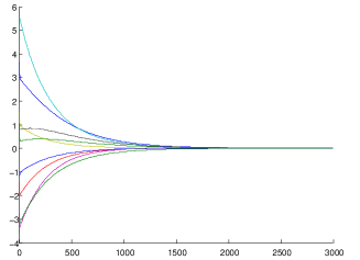
Figure 1: Trajectories of the interconnected system with periodic sampling

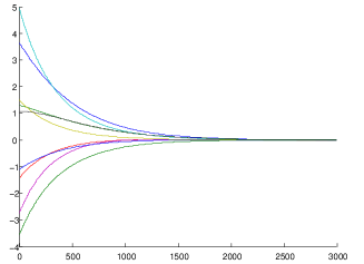
Figure 2: Trajectories of the interconnected system with event-triggering

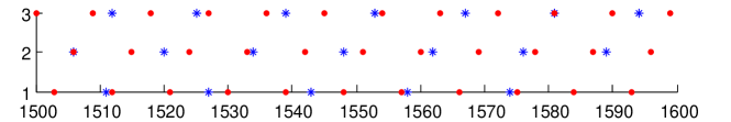
Figure 3: 33 periodic (red dots) and 22 (blue stars) events at the beginning of the simulation

Figure 4: 34 (red dots) periodic and 19 (blue stars) events in the middle of the simulation

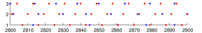
Figure 5: 34 periodic (red dots) and 21 (blue stars) events at the end of the simulation

To illustrate the feasibility of our approach we simulated the interconnection of three linear systems of dimension three. The entries of the system matrices are drawn randomly from a uniform distribution on the open interval $(-5,5)$. We repeat this procedure until the spectral radius of the corresponding matrix $G$ is less than one.
In Figure 2 new information is sampled every three units of time. Which system has to transmit information is decided by a round robin protocol (i.e., first system one, than system two, system three and again system one and so on).
In Figure 2 our event-triggered sampling scheme is used.
Over the range of $3000$ units of time the system with periodic sampling transmitted $1000$ new information, whereas in our scheme the events were triggered only $595$ times. By looking at Figure 2 and Figure 2 it seems like the periodic sampled system converges a bit faster. Indeed, the systems state norm of the event-triggered system at time $3000$ is already reached by the periodic sampled system after $2486$ (i.e., $828$ periodic samplings) units of time. But still the number of triggered events ($595$) is smaller than the number of periodic events ($828$).
A representation of how the the different systems (1,2, or 3) sample their state is depicted in Figures 4-5. The first picture shows the sampling behavior at the beginning ($t\in[0,100]$) of the simulation. The other two are from the middle ($t\in[1500,1600]$) and the end ($t\in[2800,2900]$) of the simulation, respectively. There is a small overshoot for some of the trajectories in Figure 2. This behavior cannot be seen in Figure 2, because in the event-triggered implementation information is transmitted more frequently at the beginning by systems 2 and 3, whereas in the periodic implementation transmission starts (for systems 2 and 3) a few samples later, as can be seen in Figure 4. The reason for this is that we set $\hat{x}=0$ instead of initializing $e_{0}=0$. This is another possibility of initializing the controller (and hence the initial error) than the one described in Remark 2.

7 A nonlinear example

The following interconnection of $N=2$ subsystems

$$\begin{array}[]{rcl}\dot{x}_{1}&=&x_{1}x_{2}+x_{1}^{2}u_{1}\\ \dot{x}_{2}&=&x_{1}^{2}+u_{2}\end{array}$$

is considered under the assumption that each controller can only access the state of the system it controls. The control laws are chosen accordingly as

$$u_{1}=-(x_{1}+e_{1})\;,\;u_{2}=-k(x_{2}+e_{2})\;,\;k>0\;.$$

Let $V_{i}(x_{i})=\frac{1}{2}x_{i}^{2}$ for $i=1,2$. Then

$$\dot{V}_{1}(x_{1}):=\nabla V_{1}(x_{1})(-x_{1}^{3}+x_{1}x_{2}-x_{1}^{2}e_{1})\leq x_{1}^{2}(-\frac{1}{2}x_{1}^{2}+|x_{2}|+\frac{1}{2}e_{1}^{2})$$ (20)

from which we can deduce

$$\frac{1}{4}x_{1}^{2}\geq|x_{2}|+\frac{1}{2}e_{1}^{2}\quad\Rightarrow\quad\dot{V}_{1}(x_{1})\leq-\frac{1}{4}x_{1}^{4}\,.$$

Since the left-hand side of the implication is in turn implied by $V_{1}(x_{1})\geq\max\{\sqrt{32V_{2}(x_{2})},2e_{1}^{2}\}$, this shows that the first subsystem fulfills Assumption 1 with

$$\mu_{1}=\max\;,\;\gamma_{11}(r)=0\;,\;\gamma_{12}(r)=\sqrt{32r}\;,\;\eta_{11}(r)=2r^{2}\;,\;\eta_{12}(r)=0\;.$$ (21)

Similarly

$$\dot{V}_{2}(x_{2}):=\nabla V_{2}(x_{2})(x_{1}^{2}-kx_{2}-ke_{2})\leq|x_{2}|(-k|x_{2}|+x_{1}^{2}+k|e_{2}|)$$

and therefore

$$V_{2}(x_{2})\geq\max\{\frac{32}{k^{2}}V_{1}^{2}(x_{1}),8e_{2}^{2}\}\quad\Rightarrow\quad\dot{V}_{2}(x_{2})\leq-\frac{k}{2}x_{2}^{2}\;,$$

i.e. the second subsystem satisfies Assumption 1 with

$$\mu_{2}=\max\;,\;\gamma_{21}(r)=\frac{32}{k^{2}}r^{2}\;,\;\gamma_{22}(r)=0\;,\;\eta_{21}(r)=0\;,\;\eta_{22}(r)=8r^{2}\;.$$ (22)

As discussed in Section 4, in the case of $N=2$ the $\Omega$-path can be chosen as $\sigma_{1}={\rm Id}$ and $\gamma_{21}<\sigma_{2}<\gamma_{12}^{-1}$. Provided that $k>32$, one can set $\sigma_{2}(r)=\overline{\sigma}^{2}r^{2}$, with $\overline{\sigma}^{2}\in(\frac{32}{k^{2}},\frac{1}{32})$. If $\varphi\in({\cal K}_{\infty}\cup\{0\})^{N\times N}$ is additionally chosen as

$$\varphi_{11}(r)=\sqrt{32}\overline{\sigma}r\;,\;\varphi_{12}\equiv\varphi_{21}\equiv 0\;,\;\varphi_{22}(r)=\frac{32}{k^{2}}r^{2}\;,$$

then Assumption 2 is satisfied. In view of the choice of $\sigma$, $\mu$ and $\varphi$, the requirement (6) boils down to the condition $\Gamma_{\mu}(\sigma(r))<\sigma(r)$ which is equivalent to the small-gain condition $\gamma_{12}\circ\gamma_{21}<{\rm Id}$ (see Section 4). This small-gain condition is fulfilled by the choice of $k$, since $\gamma_{12}\circ\gamma_{21}(r)=\frac{32}{k}r$. Hence Theorem 2 applies and provides an expression for the functions $\chi_{i}$ used in the event-triggered implementation of the control laws. The functions are given explicitly by

$$\chi_{1}(r):=\frac{1}{\sqrt{8}\overline{\sigma}}r^{2},\quad\chi_{2}(r):=\frac{\overline{\sigma}^{2}k^{2}}{4}r^{2}\;.$$

Simulation results for the initial condition $x_{1}(0)=-4,\,x_{2}(0)=3,\,\hat{x}_{1}(0)=-4$ and $\hat{x}_{2}(0)=3$ can be found for $t\in[0,0.5]$ in Figures 7–9.
The trajectory of the first system is given in blue and for the second system in green. The input is calculated using the red and turquoise values accordingly.
Figure 9 shows the event triggering scheme from Theorem 3. After $0.5$ seconds $12$ events were triggered. Recall that we start with $e(0)=0$. This initialization is not counted as an event. The shortest time between two events is $0.0155$ seconds. In Figure 7 we used a periodic sampling scheme with a sampling period of $0.0155$ seconds leading to a total of $66$ samples. Compared to the event triggering scheme no major improvement in the performance of the closed loop system can be recognized. Although in the periodically sampled system more than five times the amount of information was transmitted.
If we use a Round Robin protocol with $12$ periodic samples as in Figure 7 the sampling scheme is not able to stabilize the system.

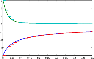
Figure 6: Trajectories of the interconnected system with periodic sampling (66 samples)

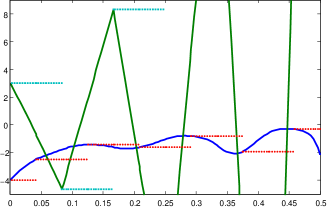
Figure 7: Trajectories of the interconnected system with periodic sampling (12 samples Round Robin)

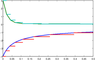
Figure 8: Trajectories of the interconnected system with event-triggered sampling (12 events)

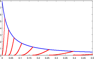
Figure 9: Lyapunov function and $\chi_{2}(\|e_{2}\|)$ for the second subsystem

In Figure 9 the Lyapunov function for the second subsystem together with $\chi_{2}(\|e_{2}\|)$ is plotted. Every time the red curve (the error function) hits the blue line, the error is reset to zero.

8 On Zeno-free distributed event-triggered control

The aim of this section is to show that it is possible to design distributed event-triggered control schemes for which the accumulation of the sampling times in finite time does not occur. The focus is again on the system (1), namely:

$$\begin{array}[]{rcl}\dot{x}_{i}&=&f_{i}(x,g_{i}(x+e))\;.\end{array}$$ (23)

We present two different approaches for a Zeno free event-triggered control scheme. The first is based on a practical ISS-Lyapunov assumption whereas the second tries to lower the amount of event-triggering by reducing unneeded information transmissions.

8.1 Practical Stabilization

Here we adopt a slight variation of the input-to-state stability property from Assumption 1.

Assumption 3

For $i\in\mathcal{N}$, there exist a differentiable function $V_{i}:\mathbb{R}^{n_{i}}\to\mathbb{R}_{+}$, and class-${\cal K}_{\infty}$ functions $\alpha_{i1},\alpha_{i2}$ such that

$$\alpha_{i1}(||x_{i}||)\leq V_{i}(x_{i})\leq\alpha_{i2}(||x_{i}||)\;.$$

Moreover there exist functions $\mu_{i}\in{\rm MAF}_{2N}$, $\gamma_{ij},\eta_{ij}\in{\cal K}_{\infty}$, for $j\in\mathcal{N}$, positive definite functions $\alpha_{i}$ and positive constants $c_{i}$, for $i\in\mathcal{N}$, such that

$$V_{i}(x_{i})\geq\max\{\mu_{i}(\gamma_{i1}(V_{1}(x_{1})),\ldots,\gamma_{iN}(V_{N}(x_{N})),\eta_{i1}(||e_{1}||),\ldots,\eta_{iN}(||e_{N}||)),c_{i}\}\\ \Rightarrow\nabla V_{i}(x_{i})f_{i}(x,g_{i}(x+e))\leq-\alpha_{i}(||x_{i}||)\;.$$ (24)

Remark 6

Systems satisfying Assumption 3 are usually referred to as input-to-state practically stable (ISpS) ([14]).

We now state a new version of Theorem 2 for system (23).

Theorem 4

Let Assumptions 2 and 3 hold. Let $V(x)=\max_{i\in{\cal N}}\sigma_{i}^{-1}(V_{i}(x_{i}))$. Assume that for each $j\in{\cal N}$ ,

$$\max\{\sigma_{j}^{-1}(V_{j}(x_{j})),c_{j}\}\geq\hat{\eta}_{j}(\|e_{j}\|)\;,$$ (25)

where

$$\hat{\eta}_{j}=\max_{i\in Z(j)}\varphi^{-1}_{ij}\circ\eta_{ij}\;.$$ (26)

Then there exists a positive definite $\alpha:\mathbb{R}_{+}\rightarrow\mathbb{R}_{+}$ such that

$$\langle p,f(x,g(x+e))\rangle\leq-\alpha(||x||),\;\forall p\in\partial V(x)\;,$$

for all $x=(x_{1}^{\top}\,x_{2}^{\top}\,\ldots\,x_{N}^{\top})^{\top}\;\in\;\{x:V(x)\geq\hat{c}:=\max_{i}\{c_{i},\sigma_{i}^{-1}(c_{i})\}\}$, where

$$f(x,g(x+e))=\left(\begin{array}[]{c}f_{1}(x,g_{1}(x+e))\\ \ldots\\ f_{N}(x,g_{N}(x+e))\\ \end{array}\right)\;.$$

Proof: Let ${\cal N}(x)\subseteq{\cal N}$ be the indices $i$ such that $V(x)=\sigma_{i}^{-1}(V_{i}(x_{i}))$.
Take any pair of indices $i,j\in{\cal N}$. By definition, $V(x)\geq\sigma_{j}^{-1}(V_{j}(x_{j}))$ and

$$\gamma_{ij}(\sigma_{j}(V(x)))\geq\gamma_{ij}(V_{j}(x_{j}))\;.$$ (27)

Let $i\in{\cal N}(x)$. Then by Assumption 2, we have:

$$V_{i}(x_{i})=\sigma_{i}(V(x))>\\ \mu_{i}(\gamma_{i1}(\sigma_{1}(V(x))),\ldots,\gamma_{iN}(\sigma_{N}(V(x))),\varphi_{i1}(V(x)),\ldots,\varphi_{iN}(V(x)))\;.$$ (28)

Bearing in mind (27), we also have

$$V_{i}(x_{i})=\sigma_{i}(V(x))>\\ \mu_{i}(\gamma_{i1}(V_{1}(x_{1})),\ldots,\gamma_{iN}(V_{N}(x_{N})),\varphi_{i1}(V(x)),\ldots,\varphi_{iN}(V(x)))\;.$$ (29)

Let us partition the set $\mathcal{N}:=\mathcal{P}\cup\mathcal{Q}$. The set $\mathcal{P}$ consists of all the indices $i$ for which the first part of the maximum in condition (25) holds, i.e. $i\in\mathcal{P}:\Leftrightarrow\sigma_{i}^{-1}(V_{i}(x_{i}))\geq c_{i}$; also $\mathcal{Q}:=\mathcal{N}\setminus\mathcal{P}$. For all $j\in\mathcal{P}$ we have by (25) $\sigma_{j}^{-1}(V_{j}(x_{j}))\geq\hat{\eta}_{j}(\|e_{j}\|)$ and hence using (26) (as mentioned before, the case $j\notin C(i)$ is trivial)

$$\varphi_{ij}(V(x))\geq\varphi_{ij}\circ\sigma_{j}^{-1}(V_{j}(x_{j}))\geq\varphi_{ij}\circ\hat{\eta}_{j}(\|e_{j}\|)\geq\\ \varphi_{ij}\circ\varphi^{-1}_{ij}\circ\eta_{ij}(\|e_{j}\|)=\eta_{ij}(\|e_{j}\|)\,.$$ (30)

Assume now that $V(x)\geq\hat{c}$. For all $j\in\mathcal{Q}$ we have by (25) $c_{j}\geq\hat{\eta}_{j}(\|e_{j}\|)$ and so

$$\varphi_{ij}(V(x))\geq\varphi_{ij}(\hat{c})\geq\varphi_{ij}(c_{j})\geq\varphi_{ij}\circ\hat{\eta}_{j}(\|e_{j}\|)\geq\eta_{ij}(\|e_{j}\|).$$ (31)

Combining (30) and (31) we get for all $j\in\mathcal{N}$

$$\varphi_{ij}(V(x))\geq\eta_{ij}(\|e_{j}\|)\;,$$

provided that (25) holds and that $V(x)\geq\hat{c}$. Substituting the latter in (29) yields

$$V_{i}(x_{i})=\sigma_{i}(V(x))>\\ \mu_{i}(\gamma_{i1}(V_{1}(x_{1})),\ldots,\gamma_{iN}(V_{N}(x_{N})),\eta_{i1}(||e_{1}||),\ldots,\eta_{iN}(||e_{N}||))\;.$$ (32)

Because $i\in\mathcal{N}(x)$ and $V(x)\geq\hat{c}=\max_{i}\{c_{i},\sigma_{i}^{-1}(c_{i})\}$, we have
$V(x)=\sigma_{i}^{-1}(V_{i}(x_{i}))\geq\hat{c}\geq\sigma_{i}^{-1}(c_{i})$ and finally we conclude

$$V_{i}(x_{i})\geq c_{i}\;.$$

The latter together with (32) is the left-hand side of the implication (24). Hence, $\nabla V_{i}(x_{i})f_{i}(x,g_{i}(x+e))\leq-\alpha_{i}(||x_{i}||)$ for all $i\in{\cal N}(x)$. Now we can repeat the same arguments of the last part of the proof of Theorem 2, and conclude that for all $x$ such that $V(x)\geq\hat{c}$ and for all $p\in\partial V(x)$, $\langle p,f(x,g(x+e))\rangle\leq-\alpha(||x||)$.   

Now that we established an analog to Theorem 2 for the case of practical stability, we are able to infer stability of the closed loop event-triggered control system (3) without the assumption that Zeno behavior does not occur.

Theorem 5

Let Assumptions 2 and 3 hold. Consider the interconnected system

$$\dot{x}_{i}(t)=f_{i}(x(t),g_{i}(\hat{x}(t)))\;,\quad i\in{\cal N}\;,$$ (33)

as in (3) with triggering conditions given by

$$T_{i}(x_{i},e_{i})=\hat{\eta}_{i}(\|e_{i}\|)-\max\{\sigma^{-1}_{i}\circ V_{i}(x_{i}),\hat{c}_{i}\}\,,$$ (34)

with $\hat{\eta}_{i}$ defined in (26) for all $i\in\mathcal{N}$. Then the origin is a globally uniformly practically stable equilibrium for (33).

Proof: Here we want to adopt the same line of reasoning as in the proof of Theorem 3. To this end, we have to make sure that by the triggering conditions given by (34) no Zeno behavior is induced. Note that in between triggering events $\dot{e}(t)=-\dot{x}(t)$ for all $t\in(t_{k},t_{k+1})$ by the definition of (3). The triggering conditions $T_{i}(x_{i},e_{i})=\hat{\eta}_{i}(\|e_{i}\|)-\max\{\sigma^{-1}_{i}\circ V_{i}(x_{i}),\hat{c}_{i}\}\geq 0$ ensure that $\max\{\sigma^{-1}_{i}\circ V_{i}(x_{i}),\hat{c}_{i}\}\geq\hat{\eta}_{i}(\|e_{i}\|)$ for all positive times. Following the same reasoning of Theorem 3, with the exception that we have to replace the application of Theorem 2 with the application of Theorem 4, one proves that $V(x(t))$ is decreasing along the solution $x(t)$ on its domain of definition. Hence, $x(t)$ is bounded on its domain of definition. Since $\max\{\sigma^{-1}_{i}\circ V_{i}(x_{i}(t)),\hat{c}_{i}(t)\}\geq\hat{\eta}_{i}(\|e_{i}(t)\|)$, then also $e(t)$ is bounded and so is $\hat{x}(t)=x(t)+e(t)$. As $e_{j}(t_{k}^{+})=0$ for each index $j$ which triggered an event and $\dot{e}(t)$ is bounded in between events ($\dot{e}(t)=-\dot{x}(t)=-f(x(t),g(\hat{x}(t)))$), the time when the next event will be triggered by system $j$ is bounded away from zero because the time it takes $e_{j}$ to evolve from zero to $c_{j}$ is bounded away from zero. Hence, either there is a finite number of times $t_{k}$ or $t_{k}\rightarrow\infty$ as $k$ goes to infinity. The solution $x(t)$ is then defined for all positive times and Theorems 3 and 4 allow us to conclude.   

In hybrid systems, the practice of avoiding Zeno effects while retaining stability in the practical sense is referred to as temporal regularization (see [11], p. 73, and references therein). Here, the regularization is achieved via a notion of practical ISS. In the context of event-triggered ${\cal L}_{2}$-disturbance attenuation control for linear systems temporal regularization is studied in [10].

8.2 Parsimonious Triggering

In Section 8.1 a way to exclude the occurrence of Zeno behavior for the price of practical stability rather than asymptotic stability was shown. Here we want to provide a way to exclude the Zeno effect by introducing a new triggering scheme, but still achieving asymptotic stability. The main idea behind the new triggering scheme, which will be introduced in Theorem 7 is that if the error of the $i$th subsystem is bigger than its Lyapunov function but still small compared to the Lyapunov function of the overall system, no transmission of the $i$th subsystem is needed.
For future use we need also a slight variation of Theorem 2. Here we exploit the fact that we can either compare each state to its corresponding error (as in Theorem 2) or each error to the Lyapunov function of the overall system as shown in the next theorem.

Theorem 6

Let Assumptions 1 and 2 hold. Let $V(x)=\max_{i\in{\cal N}}\sigma_{i}^{-1}(V_{i}(x_{i}))$ and, for each $j\in{\cal N}$, define:

$$\hat{\eta}_{j}=\max_{i\in{Z(j)}}\varphi_{ij}^{-1}\circ\eta_{ij}\;.$$ (35)

Then there exist a positive definite $\alpha\,:\,\mathbb{R}_{+}\rightarrow\mathbb{R}_{+}$ such that the condition

$$V(x)\geq\hat{\eta}_{j}(\|e_{j}\|),\;\forall j\in\mathcal{N}$$ (36)

implies

$$\langle p,f(x,g(x+e))\rangle\leq-\alpha(||x||),\;\forall p\in\partial V(x)\;.$$

Proof: The proof follows by a slight modification of the proof of Theorem 2.
For each $x$, let $\mathcal{N}(x)\subset\mathcal{N}$ be set of indices for which $V(x)=\sigma_{i}^{-1}(V_{i}(x_{i}))$.
It is sufficient to show that for all $i\in\mathcal{N}(x),\,j\in\mathcal{N}$ we have $\varphi_{ij}(r)\geq\eta_{ij}(\|e_{j}\|)$, with $r=V(x)$.
First recall that for $j\notin C(i)$ the latter inequality trivially holds. So assume that $j\in C(i)$. Using (35) and (36), we have

$$\varphi_{ij}(V(x))\geq\varphi_{ij}(\hat{\eta}_{j}(\|e_{j}\|))\geq\varphi_{ij}\circ\varphi_{ij}^{-1}\circ\eta_{ij}(\|e_{j}\|)=\eta_{ij}(\|e_{j}\|)\;.$$

i.e. (12) in the proof of Theorem 2. Then the argument after (12) can be repeated word by word. By previous arguments this concludes the proof.   

A triggering condition for the $j$th subsystem which yield the validity of condition (36) would make the knowledge of the Lyapunov function $V$ of the overall system to system $j$ necessary. This would contradict our wish for a decentralized approach.
The next lemma provides a decentralized way to ensure that condition (36) holds. To this end, we give an approximation of the other states (the $W$) which will be compared to the error instead of the Lyapunov function of the overall system. Appropriately scaled, $W$ is a lower bound on the Lyapunov function of the overall system and hence can be used to check the validity of (36). The important advantage is, that this approximation can be calculated by using only local information. Before we state the next lemma, define

$$\xi^{j,x_{j}}:=\left(\xi_{1}^{\top},\dots,\xi_{j-1}^{\top},x_{j}^{\top},\xi_{j+1}^{\top},\dots,\xi_{N}^{\top}\right)^{\top}\;$$

as the vector $\xi$ where the $j$th component is replaced by $x_{j}$. The proofs of Lemma 2, 3, and 4 are postponed to the Appendix.

Lemma 2

Let Assumptions 1 and 2 hold. Let $V(x)=\max_{i\in{\cal N}}\sigma_{i}^{-1}(V_{i}(x_{i}))$. Let $d_{j}\in\mathbb{R}_{+}$ be an approximation of $\|f_{j}(x,g_{j}(x+e))\|$ with $|\|f_{j}(x,g_{j}(x+e))\|-d_{j}|\leq\tilde{\kappa}_{j}\|x_{j}\|$.
Assume that for $j\in\mathcal{N}$ there exist functions $\Theta_{j}\;:\mathbb{R}^{N}\rightarrow\mathbb{R}$ such that $V(x)\geq\hat{\eta}_{i}(\|e_{i}\|)$ for all $i\neq j$ implies

$$\Theta_{j}(\|x_{1}\|,\dots,\|x_{N}\|)\geq\|f_{j}(x,g_{j}(x+e))\|\,.$$ (37)

Define

$$W(j,x_{j},d_{j})=\min\{\max_{i\neq j}\|\xi_{i}\|\;:\;\xi\in\mathcal{A}(j,x_{j},d_{j})\}$$

with

$$\mathcal{A}(j,x_{j},d_{j})=\{\xi^{j,x_{j}}\;:\;\Theta_{j} (\|\xi_{1}\|,\dots,\|\xi_{N}\|)\geq d_{j}-\tilde{\kappa}_{j}\|x_{j}\|\}\;.$$ (38)

Then the conditions

$$W(j,x_{j},d_{j})\geq\psi_{j}^{-1}\circ\hat{\eta}_{j}(\|e_{j}\|)\quad\text{and}\quad\sigma_{j}^{-1}(V_{j}(x_{j}))\leq\hat{\eta}_{j}(\|e_{j}\|),$$ (39)

with $\psi_{j}=\max_{i\neq j}\sigma_{i}^{-1}\circ\alpha_{i1}$ imply

$$V(x)\geq\hat{\eta}_{j}(\|e_{j}\|)\;.$$

Remark 7

Lemma 2 presents a way of approximating the norm of the other states influencing the dynamics of a single subsystem. To this end an approximation of the derivative is used. Another possibility for achieving this goal would be to construct an observer, which gives an approximation of the inputs (the other states) by observing the dynamics of a single subsystem.

Before we can state another event-triggering scheme, which does not induce Zeno behavior we have to formulate the observation that if Zeno behavior occurs, one of the states has to approach the equilibrium.

Lemma 3

Consider a large scale system with triggered control of the form (3) satisfying Assumptions 1 and 2. Let $\chi_{i},\,i\in\mathcal{N}$ be given by (7). Consider the triggering conditions given by

$$T_{i}(x_{i},e_{i})=\chi_{i}(\|e_{i}\|)-V_{i}(x_{i})\;.$$

If for a given initial condition $x_{0}$ the triggering scheme $T_{i^{*}}$ induces Zeno behavior, then the corresponding solution

$$x_{i^{*}}(t_{k})\rightarrow 0\;.$$

The next lemma provides an inequality for the state and the corresponding dynamics. Besides the rather technical nature of Lemma 4, together with Lemma 3 it forms the basis to be able to compare the $i$th state to the rest of the states as will be seen in Theorem 7.

Lemma 4

Consider system

$$\dot{x}=f(x,g(x+e))$$ (40)

as in (3). If there are triggering instances $t_{k}\to t^{*}$ for $k\to\infty$ and an index $i$ such that $x_{i}(t_{k})\to 0$, then for all $M>0$ there exists a $k^{*}\in\mathbb{N}$ such that for some $k\geq k^{*}$

$$\frac{\|x_{i}(t_{k+1})-x_{i}(t_{k})\|}{t_{k+1}-t_{k}}>M\|x_{i}(t_{k+1})\|.$$

It is of interest to note the following immediate corollary.

Corollary 1

Under the conditions of Lemmas 3 and 4, assume that the functions $\Theta_{j}$ from Lemma 2 satisfying (37) may be chosen to be Lipschitz and so that $\Theta_{i}(0,\dots,0)=0$ holds. Consider an initial condition $x(0)=x_{0}\neq 0$. If there is Zeno behavior at $t^{*}$, i.e. if there are triggering instances $t_{k}\to t^{*}$, then for the overall state $x$ of (40)

$$x(t_{k})\not\to 0\quad\text{ as }k\to\infty\,.$$ (41)

Proof: We first exclude that there is a $s^{*}\in[0,t^{*})$ such that $x(s^{*})=0$. Otherwise choose Lipschitz constants $L_{i}$ for $\Theta_{i}$ valid on the compact set $\{x(s)\;;\;s\in[0,s^{*}]\}$ and note that we have for each $i$ almost everywhere on $[0,s^{*}]$

$$\|\dot{x}_{i}(t)\|=\|f_{i}(x(t),g_{i}(x(t)+e(t)))\|\\ \leq\Theta_{i}(\|x_{1}(t)\|,\ldots,\|x_{N}(t)\|)\leq L_{i}\|x(t)\|\;.$$ (42)

Note that we can use $\Theta_{i}$ as a bound for the dynamics as in (37), because the validity of $V_{i}(x_{i})\geq\chi_{i}(\|e_{i}\|)$ for all $i$ trivially implies $V(x)\geq\hat{\eta}_{i}(\|e_{i}\|)$.
As (42) is true for all $i$, this implies $\|\dot{x}(t)\|\leq L\|x(t)\|$ for $L$ sufficiently large and almost all $t\in[0,s^{*}]$. It follows that $\|x(s^{*})\|\geq e^{-Ls^{*}}\|x(0)\|>0$, so that $x(s^{*})\neq 0$.
If $x(t_{k})\to 0$, then $x(t)\to 0$ for $t\nearrow t^{*}$. Hence for each $i$, and $k$ sufficiently large we have that (42) holds almost everywhere on $(t_{k},t^{*})$. As in the first part of the proof it follows that $\|x(t^{*})\|\geq e^{-L(t^{*}-t_{k})}\|x(t_{k})\|>0$, because by the first step of the proof $x(t_{k})\neq 0$. This contradicts the assumption that $x(t_{k})\to 0$.   

The rest of this section is devoted to constructing an event-triggered control scheme which ensures that Condition (36) holds.
From Lemma 3 we know that if Zeno behavior occurs, then one of the subsystems approaches the origin in finite time. Corollary 1 shows that under certain regularity assumptions, a number of subsystems do not converge to $0$ as we approach the Zeno point. Hence, from a certain time on, the Lyapunov function corresponding to the subsystem which tends to the origin does not contribute to the Lyapunov function for the overall system. As a consequence no information transfer from this subsystem is necessary using parsimonious triggering. This observation is made rigorous in the rest of the section.
In the next theorem we use the triggering condition as in Theorem 3 but we add another triggering condition $T_{i2}$, which checks whether the $i$th subsystem contributes to the Lyapunov function of the overall system. It does so by comparing the local error of system $i$ with the approximation $W$ of the other states as described in Lemma 2. The main idea is that if the dynamics of the $i$th system is large compared to its own state, other states must be large. As the correct value of the dynamics is not known to system $i$, an approximation of $\|\dot{x}_{i}\|$ is used.
As the aim is to use only local information, we will use the difference quotients to approximate the size of the derivative at the triggering points. Furthermore, we do not wish to assume that all subsystems are aware of all triggering events. Hence in the following we will use the notation $t_{k}^{i}$ to denote those triggering events initiated by system $i$. We define

$$d_{i}(t)=\frac{\|x_{i}(t)-x_{i}(t_{{k-1}}^{i})\|}{t-t_{{k-1}}^{i}}$$ (43)

as the difference quotient approximating $\|\dot{x}_{i}(t)\|$ after the triggering event $t_{k-1}^{i}$.
Adding the new triggering condition that uses (43) allows us to exclude the occurrence of Zeno behavior. A discussion about the new triggering condition can be found in Remark 8 and 9.

Theorem 7

Consider a large scale system with triggered control of the form (3) satisfying Assumptions 1 and 2. Let $V(x)=\max_{i\in\mathcal{N}}\sigma_{i}^{-1}(V_{i}(x_{i}))$. Define

$$T_{i1}(x_{i},e_{i})=\chi_{i}(\|e_{i}\|)-V_{i}(x_{i})$$

with $\chi_{i}$ as in Theorem 3 and

$$T_{i2}(x_{i},e_{i},d_{i})=\psi_{i}^{-1}\circ\hat{\eta}_{i}(\|e_{i}\|)-W(i,x_{i},d_{i})\;,$$

where $\psi_{i},\,W(i,x_{i},d_{i})$ and $\hat{\eta}_{i}$ are defined as in Lemma 2. Furthermore, assume that for all $i\in\mathcal{N}$ the $\Theta_{i}$ from Lemma 2 and $\psi_{i}^{-1}\circ\hat{\eta}_{i}$ are Lipschitz with Lipschitz constant $L_{i}$ respectively $K_{i}$ and that $\Theta_{i}(0,\dots,0)=0$ holds.
Consider the interconnected system

$$\dot{x}_{i}(t)=f_{i}(x(t),g_{i}(\hat{x}(t)))\;,\quad i\in{\cal N}\;,$$ (44)

as in (3) with triggering conditions given by

$$T_{i}(x_{i},e_{i},d_{i})=\min\{T_{i1}(x_{i},e_{i}),T_{i2}(x_{i},e_{i},d_{i})\}\,,$$ (45)

for all $i\in\mathcal{N}$. Then the origin is a globally uniformly asymptotically stable equilibrium for (44), if there are constants $\kappa_{j}>0,\;j\in{\cal N}$ such that at the triggering times $t_{k}$, which are implicitly defined by (44) and (45) as described in Section 3, the following condition is satisfied:

$$|\|\dot{x}_{j}(t_{k}^{j})\|-d_{j}(t_{k}^{j})|\leq\kappa_{j}\|x_{j}(t_{k}^{j})\|$$ (46)

where $d_{j}(t_{k_{j}}^{j})$ is defined by (43). In particular, no Zeno behavior occurs.

Proof: Before we can use Theorem 3 respectively Theorem 6 to conclude stability, we have to exclude the occurrence of Zeno behavior. First note that condition (45) triggers an event if and only if $T_{i1}\geq 0$ and $T_{i2}\geq 0$ respectively condition (8) and (36) are violated. Now assume that the $j$th subsystem induces Zeno behavior. For simplicity, we omit the index $j$ of the triggering times $t_{k}^{j}$. Hence, let $t_{k}$ the triggering times of the $j$th subsystem and $t^{*}=\lim_{k\rightarrow\infty}t_{k}$ the finite accumulation point. From Lemma 3 we know that the $j$th subsystem has to approach the equilibrium, i.e. $\lim_{t_{k}\rightarrow t^{*}}x_{j}(t_{k})=0$. Lemma 4 tells us that for all $M$ there exists a $k^{*}$ such that for some $k\geq k^{*}$

$$\frac{\|x_{j}(t_{k})-x_{j}(t_{k-1})\|}{t_{k}-t_{k-1}}>M\|x_{j}(t_{k})\|\;.$$ (47)

As discussed in the proof of Lemma 2, the full state $x\in A\subset\mathcal{A}$. But the knowledge of $x$ is not available to a single subsystem. Hence, we take $\xi(t_{k})\in\mathcal{A}(j,x_{j}(t_{k}),d_{j}(t_{k}))$ as in the definition of $W$ as an approximation for the states of the other subsystems. For this $\xi$ we can deduce together with the Lipschitz continuity of $\Theta_{j}$ and (47)

$$L_{j}\max_{i\neq j}\{\|\xi_{i}(t_{k})\|,\|x_{j}(t_{k})\|\}\geq\Theta_{j}(\|\xi_{1}\|,\dots,\|x_{j}\|,\dots,\|\xi_{N}\|)\geq\\ \frac{\|x_{j}(t_{k})-x_{j}(t_{k-1})\|}{t_{k}-t_{k-1}}-\kappa_{j}\|x_{j}(t_{k})\|\geq(M-\kappa_{j})\|x_{j}(t_{k})\|\;.$$ (48)

And hence for the $k$ given in (47)

$$\max_{i\neq j}\{\|\xi_{i}(t_{k})\|,\|x_{j}(t_{k})\|\}>\frac{M-\kappa_{j}}{L_{j}}\|x_{j}(t_{k})\|\;.$$ (49)

Now choose

$$M>\max\{\kappa_{j}+L_{j},\kappa_{j}+L_{j}K_{j}\}\;,$$ (50)

where $K_{j}$ is the Lipschitz constant of $\psi_{j}^{-1}\circ\hat{\eta}_{j}$. From Lemma 4 we know that this choice of $M$ yields a $k^{*}$ such that we can conclude together with (49) $\max_{i\neq j}\{\|\xi_{i}(t_{k})\|,\|x_{j}(t_{k})\|\}=\max_{i\neq j}\|\xi_{i}(t_{k})\|$ for some $k\geq k^{*}$. For this $k$ we want to show that the corresponding $t_{k}$ is not a triggering time.
To this end we use (48) and (47) to get

$$\max_{i\neq j}\|\xi_{i}(t_{k})\|\geq\frac{1}{L_{j}}(1-\frac{\kappa_{j}}{M})\frac{\|x_{j}(t_{k})-x_{j}(t_{k-1})\|}{t_{k}-t_{k-1}}\;.$$ (51)

Note that for the $j$th subsystem (51) is true for all $\xi\in\mathcal{A}$ and therefore by the definition of $W$

$$W(j,x_{j},d_{j})\geq\frac{1}{L_{j}}(1-\frac{\kappa_{j}}{M})\frac{\|x_{j}(t_{k})-x_{j}(t_{k-1})\|}{t_{k}-t_{k-1}}\;.$$

Using the latter inequality and the Lipschitz constant for $\psi_{j}^{-1}\circ\hat{\eta}_{j}$ we can bound $T_{j2}$ by

$$T_{j2}\leq K_{j}\|e_{j}(t_{k})\|-\frac{1}{L_{j}}(1-\frac{\kappa_{j}}{M})\frac{\|x_{j}(t_{k})-x_{j}(t_{k-1})\|}{t_{k}-t_{k-1}}\,.$$

From the definition of $e_{j}(t_{k})=x_{j}(t_{k-1})-x_{j}(t_{k})$ we arrive at

$$T_{j2}\leq K_{j}\|x_{j}(t_{k})-x_{j}(t_{k-1})\|-\frac{1}{L_{j}}(1-\frac{\kappa_{j}}{M})\frac{\|x_{j}(t_{k})-x_{j}(t_{k-1})\|}{t_{k}-t_{k-1}}\,.$$

We may assume that $k^{*}$ is sufficiently large so that $t_{k}-t_{k-1}<M^{-1}$ for all $k\geq k^{*}$. Together with (50) we obtain

$$K_{j}<\frac{1}{L_{j}(t_{k}-t_{k-1})}(1-\frac{\kappa_{j}}{M})$$

and hence $T_{j2}<0$ in contradiction to the assumption that $t_{k}$ is a triggering time. Because the only further assumption on the solution of (44) and (45) is the occurrence of Zeno behavior, the aforementioned contradiction shows that Zeno behavior cannot occur.
To conclude stability define

$$I(x,e):=\{j\in\mathcal{N}\;:\;V_{j}(x_{j})\geq\chi_{j}(\|e_{j}\|)\}\,,$$

$$J(x,e):=\{j\in\mathcal{N}\;:\;V(x)\geq\hat{\eta}_{j}(\|e_{j}\|)\}\,,$$

and

$$\mathcal{J}(x,e):=\{j\in\mathcal{N}\;:\;\psi_{j}(W(j,x_{j},d_{j}))\geq\hat{\eta}_{j}(\|e_{j}\|)\}\;.$$

Note that the triggering condition $T_{j}$ ensures that $j\in I\cup\mathcal{J}$. For $j\in I$ we can use exactly the same reasoning as in Theorem 3.
Lemma 2 tells us that from $j\not\in I$ and $j\in\mathcal{J}$ we can deduce $j\in J$. For the case $j\in J$ we can adopt nearly the same reasoning as in Theorem 3. Only the reasoning for the existence of a Lyapunov function for the overall system changes. In Theorem 3 it can be deduced from Theorem 2 whereas here we have to use Theorem 6 to conclude the existence of a Lyapunov function. The rest of the proof can be copied word by word from Theorem 3. This ends the proof.   

Remark 8

The advantage of parsimonious triggering is twofold. First it allows us to exclude the occurrence of Zeno behavior and second it may lead to fewer transmissions compared to the triggering condition given in Theorem 3. Compared to Theorem 5 where the same goal is achieved by the notion of practical stability, here we still achieve asymptotic stability, but we have to place more technical assumptions on the involved class $\mathcal{K}$ estimates.
Note that the set of indices $j\in\mathcal{N}$ for which condition (8) holds is a subset of those for which (36) holds (in other words $I(x,e)\subset J(x,e)$). But we cannot check condition (36) locally.
Because of the conservatism we introduce by using $T_{i2}$ instead of (36), triggering condition $T_{i}$ still makes sense.
In a practical implementation $T_{i1}$ should be checked first, before $T_{i2}$ is checked, because of the conservatism of $T_{i2}$ and the possible cumbersome calculation of $W$.

Remark 9

One possible drawback of the triggering condition given in Theorem 7 is that the condition on the approximation $d_{j}$ as in (46) might be too demanding. First note, that if $t_{k}-t_{k-1}$ is sufficiently small, (46) trivially holds true, because $d_{j}$ is the difference quotient. As $x_{i}$ approaches zero, it could happen that the difference $t_{k}-t_{k-1}$ does not decline fast enough to ensure that (46) holds. A way to overcome this issue would be to adjust condition $T_{i2}$ in such a way that it always tries to trigger an event as soon as it cannot be guaranteed that the approximation $d_{j}$ satisfies (46).

9 Conclusion

We presented event-triggered sampling schemes for controlling interconnected systems. Each system in the interconnection decides when to send new information across the network independently of the other systems. This decision is based only on each system’s own state and a given Lyapunov function. Stability of the interconnected system is inferred by the application of a nonlinear small-gain condition. The feasibility of our approach is presented with the help of numerical simulations. To prevent the accumulation of the sampling times in finite time, we propose two variations of the event-triggered sampling-scheme. The first is based on the notion of input-to-state practical stability, whereas the second compares the local error to an approximation of the Lyapunov function of the overall system to guarantee stability of the interconnected system.

Appendix A Appendix

A.1 Proof of Lemma 2

Proof: For later use define

$$A(j,x_{j},e_{j},\dot{x}_{j})=\{\xi^{j,x_{j}}\;:\;\exists\;\epsilon\in\mathbb{R}^{n_{i}}\text{ s.t. }f_{j}(\xi^{j,x_{j}},g_{j}(\xi^{j,x_{j}}+\epsilon^{j,e_{j}}))=\dot{x}_{j}\text{ and }\\ V(\xi^{j,x_{j}})\geq\hat{\eta}_{i}(\|\epsilon_{i}\|)\;\forall i\neq j\}\;.$$ (52)

The set $A(j,x_{j},e_{j},\dot{x}_{j})$ describes the set of all $\xi^{j,x_{j}}$ for which a pair $(\xi^{j,x_{j}},\epsilon^{j,e_{j}})$ exists that fulfills the right hand side of the $j$th subsystem for a given $\dot{x}_{j},x_{j},e_{j}$ and for which $V(\xi^{j,x_{j}})\geq\hat{\eta}_{j}(\|\epsilon_{i}\|)$ for all $i\neq j$ hold. As the system’s state satisfies the dynamics, it holds that $x\in A$.
Before we proceed, we want to show that $A(j,x_{j},e_{j},\dot{x}_{j})\subset\mathcal{A}(j,x_{j},d_{j})$. To this end take a $\xi\in A(j,x_{j},e_{j},\dot{x}_{j})$. Hence we have $f_{j}(\xi^{j,x_{j}},g_{j}(\xi^{j,x_{j}}+\epsilon^{j,e_{j}}))=\dot{x}_{j}$. Taking the norm and using (37) yields

$$\Theta_{j}(\|\xi_{1}\|,\dots,\|\xi_{n}\|)\geq\|f_{j}(\xi^{j,x_{j}},g_{j}(\xi^{j,x_{j}}+\epsilon^{j,x_{j}}))\|=\|\dot{x}_{j}\|\geq d_{j}-\tilde{\kappa}_{j}\|x_{j}\|\,,$$

where the last inequality follows from the condition on the approximation for $\|\dot{x}_{j}\|$. And we can conclude $A(j,x_{j},e_{j},\dot{x}_{j})\subset\mathcal{A}(j,x_{j},d_{j})$.
From condition (39) we can deduce

$$\psi_{j}^{-1}\circ\hat{\eta}(\|e_{j}\|)\leq W(j,x_{j},d_{j})=\min\{\max_{i\neq j}\|\xi_{i}\|\;:\;\xi\in\mathcal{A}(j,x_{j},d_{j})\}\leq\\ \min\{\max_{i\neq j}\|\xi_{i}\|\;:\;\xi\in A(j,x_{j},e_{j},\dot{x}_{j})\}\leq\max_{i\neq j}\|x_{i}\|\;.$$ (53)

The second inequality follows from $A(j,x_{j},e_{j},\dot{x}_{j})\subset\mathcal{A}(j,x_{j},d_{j})$ and the last can be deduced from $x\in A$. Now we can rewrite (53) to get

$$\hat{\eta}_{j}(\|e_{j}\|)\leq\psi_{j}(\max_{i\neq j}\|x_{i}\|)\;.$$

With the help of (39) and the definition of $\psi_{j}$ we arrive at

$$\sigma_{j}^{-1}(V_{j}(x_{j}))\leq\hat{\eta}_{j}(\|e_{j}\|)\leq\max_{i\neq j}\sigma_{i}^{-1}\circ\alpha_{1i}(\|x_{i}\|)\leq\max_{i\neq j}\sigma_{i}^{-1}(V_{i}(x_{i}))\,,$$

where the last inequality follows from Assumption 1. Considering the first and the last term in the chain of inequalities above it is easy to see that the $j$th subsystem does not contribute to the Lyapunov function of the overall system and we conclude $\max_{i\neq j}\sigma_{i}^{-1}(V_{i}(x_{i}))=\max_{i\in\mathcal{N}}\sigma_{i}^{-1}(V_{i}(x_{i}))=V(x)$ and the proof is complete.   

A.2 Proof of Lemma 3

Proof: Denote $t^{*}=\lim_{k\rightarrow\infty}t_{k}$. By definition of the triggering condition we have for each $k$ an index $i(k)\in\mathcal{N}$ such that

$$V_{i(k)}(x_{i(k)}(t_{k}))=\chi_{i(k)}(\|e_{i(k)}(t_{k})\|)\;.$$

Choose $i^{*}\in\mathcal{N}$ such that $i(k)=i^{*}$ for infinitely many $k$. Such a $i^{*}$ exists because $\mathcal{N}$ is finite and $k$ ranges over all of $\mathbb{N}$. Let $K$ be the set of indices for which $i(k)=i^{*}$. For ease of notation let $K=\{s_{1},s_{2},\dots\}$. By Theorem 2 $V$ is a Lyapunov function for the event triggered system on the interval $[0,t^{*})$. Thus the trajectory $x_{|[0,t^{*})}$ is bounded and $e_{|[0,t^{*})}$ is bounded because $\chi_{i}(\|e_{i}(t)\|)\leq V_{i}(x_{i}(t))$ for all $i\in\mathcal{N},\,t\in[0,t^{*})$. It follows that $u_{i|[0,t^{*}))}$ is bounded and so $\dot{x}_{i}$ is bounded on $[0,t^{*})$ for all $i\in\mathcal{N}$.
Then we have by uniform continuity of $x_{i^{*}}$ on $[0,t^{*})$ that the following limit exists

$$\lim_{k\rightarrow\infty}\chi_{{i^{*}}}(\|e_{i^{*}}(s_{k})\|)=\lim_{k\rightarrow\infty}V_{i^{*}}(x_{i^{*}}(s_{k}))=V_{i^{*}}(x_{i^{*}}(t^{*})).$$ (54)

By definition $e_{i^{*}}(s_{k}^{+})=0$. By (3) we have that $\dot{e}_{i^{*}}=-\dot{x}_{i^{*}}$ almost everywhere on $(s_{k},s_{k+1})$. Since $\dot{x}_{i^{*}}$ is bounded and $s_{k+1}-s_{k}\rightarrow 0$, then condition $e_{i^{*}}(s_{k}^{+})=0$ implies that

$$e_{i^{*}}(s_{k+1})=e_{i^{*}}(s_{k}^{+})+\int_{s_{k}}^{s_{k+1}}\dot{e}_{i^{*}}(\tau)d\tau=\int_{s_{k}}^{s_{k+1}}\dot{e}_{i^{*}}(\tau)d\tau$$

which goes to $0$ for $k\rightarrow\infty$. Hence by (54) we obtain that $V_{i^{*}}(x_{i^{*}}(t^{*}))=0$. This shows the assertion.   

A.3 Proof of Lemma 4

Proof: The proof will be by contradiction. To this end assume that for some fixed $M>0$ and all $k$ sufficiently large we have

$$\|x_{i}(t_{k+1})-x_{i}(t_{k})\|\leq M(t_{k+1}-t_{k})\|x_{i}(t_{k+1})\|\;.$$ (55)

The evolution of $x_{i}$ between $t_{l}$ and $t_{k}$ for $k>l$ can be bounded by using a telescoping sum, the triangle inequality, applying (55), and a judicious addition of $0$:

$$\|x_{i}(t_{k})-x_{i}(t_{l})\|\leq\\ \sum\limits_{j=l+1}^{k-1}M(t_{j}-t_{j-1})\|x_{i}(t_{j})-x_{i}(t_{l})\|+M(t_{k}-t_{l})\|x_{i}(t_{l})\|+M(t_{k}-t_{k-1})\|x_{i}(t_{k})-x_{i}(t_{l})\|\;.$$

If we choose $D>0$ and a $k^{\prime}$ such that $0\leq\frac{1}{1-M(t_{k}-t_{k-1})}\leq D$ for all $k>k^{\prime}$, we can rewrite the latter to

$$\|x_{i}(t_{k})-x_{i}(t_{l})\|\leq\frac{1}{1-M(t_{k}-t_{k-1})}\sum\limits_{j=l+1}^{k-1}M(t_{j}-t_{j-1})\|x_{i}(t_{j})-x_{i}(t_{l})\|+\\ \frac{M(t_{k}-t_{l})}{1-M(t_{k}-t_{k-1})}\|x_{i}(t_{l})\|\;.$$

Using the discrete Gronwall inequality (see e.g., Theorem 4.1.1 from [1]) yields

$$\|x_{i}(t_{k})-x_{i}(t_{l})\|\leq\frac{M(t_{k}-t_{l})}{1-M(t_{k}-t_{k-1})}\|x_{i}(t_{l})\|+\\ \frac{1}{1-M(t_{k}-t_{k-1})}\sum\limits_{j=l+1}^{k-1}\frac{M(t_{j}-t_{l})}{1-M(t_{j}-t_{j-1})}\|x_{i}(t_{l})\|\;M(t_{j}-t_{j-1})\prod\limits_{s=j+1}^{k-1}(1+\frac{M(t_{s}-t_{s-1})}{1-M(t_{s}-t_{s-1})})\;.$$

Exploiting that $t_{k}$ is a monotone sequence, that $0\leq\frac{1}{1-M(t_{k}-t_{k-1})}\leq D$ and that $1+x\leq e^{x}$ for all $x\in\mathbb{R}$ and collapsing the telescoping sum again gives

$$\|x_{i}(t_{k})-x_{i}(t_{l})\|\leq\underbrace{(MD(t_{k}-t_{l})+M^{2}D^{2}(t_{k-1}-t_{l})^{2}e^{MD(t_{k-1}-t_{l})})}_{:=C}\|x_{i}(t_{l})\|\,.$$

Because of the finite accumulation point $t^{*}$, there exists an $k^{*}>k^{\prime}$ such that

$$\|x_{i}(t_{k})-x_{i}(t_{l})\|\leq C\|x_{i}(t_{l})\|$$

for all $k\geq l\geq k^{*}$ with $C<1$. Realizing that this contradicts $\|x_{i}(t^{*})\|=0$ finishes the proof.

References

• [1] Ravi P. Agarwal. Difference equations and inequalities: theory, methods, and applications, volume 228 of Pure and applied mathematics. Dekker, New York, 2., rev. and expanded edition, 2000.
• [2] A. D. Ames, H. Zheng, R. D. Gregg, and S. Sastry. Is There Life after Zeno? Taking Executions Past the Breaking (Zeno) Point. In Proceedings of the American Control Conference, Minneapolis, MN, pages 2652–2657, 2006.
• [3] A. Anta and P. Tabuada. To sample or not to sample: Self-triggered control for nonlinear systems. IEEE Trans. Autom. Control, 55(9):2030 – 2042, 2010.
• [4] A. Bacciotti and L. Rosier. Liapunov functions and stability in control theory. Springer Verlag, London, 2005.
• [5] F. Ceragioli. Discontinuous Ordinary Differential Equations and Stabilization. PhD thesis, Department of Mathematics, Università di Firenze, 1999.
• [6] N. Chung Siong Fah. Input-to-state stability with respect to measurement disturbances for one-dimensional systems. ESAIM, Control Optim. Calc. Var., (4):99–121, 1999.
• [7] S. Dashkovskiy, B.S. Rüffer, and F.R. Wirth. An ISS small gain theorem for general networks. Math Control Signal Syst, 19(2):93–122, 2007.
• [8] S.N. Dashkovskiy, B.S. Rüffer, and F.R. Wirth. Small gain theorems for large scale systems and construction of ISS Lyapunov functions. SIAM J. Control Optim., 48(6):4089–4118, 2010.
• [9] D.V. Dimarogonas and K.H. Johansson. Event-triggered control for multi-agent systems. In Proceedings of the IEEE Conference on Decision and Control, Shanghai, China, pages 7131–7136, 2009.
• [10] M.C.F. Donkers and W.P.M.H. Heemels. Output-based event-triggered control with guaranteed ${\cal L}_{2}$-gain and Improved Event-triggering. In Proceedings of the 49th IEEE Conference on Decision and Control, Atlanta, GA, pages 3246–3251, 2010.
• [11] R. Goebel, R. Sanfelice, and A.R. Teel. Hybrid dynamical systems. IEEE Control Systems Magazine, 29(2):28–83, 2009.
• [12] H. Ito, S. Dashkovskiy, and F. Wirth. On a small gain theorem for networks of iISS systems. In Proceedings of the IEEE Conference on Decision and Control, Shanghai, China, pages 4210–4215, 2009.
• [13] Z. P. Jiang, A. R. Teel, and L. Praly. Small-gain theorem for ISS systems and applications. Math Control Signal Syst, 7(2):95–120, 1994.
• [14] Z.P. Jiang, I.M.Y. Mareels, and Y. Wang. A Lyapunov formulation of the nonlinear small-gain theorem for interconnected ISS systems. Automatica, 32(8):1211–1215, 1996.
• [15] M. Krstic, I. Kanellakopoulos, and P.V. Kokotovic. Nonlinear and adaptive control design. John Wiley & Sons, New York, 1995.
• [16] D. Liberzon, E.D. Sontag, and Y. Wang. Universal construction of feedback laws achieving ISS and integral-ISS disturbance attenuation. Systems & Control Letters, 46(2):111–127, 2002.
• [17] T. Liu, Z.-P. Jiang, and D.J. Hill. Lyapunov-ISS cyclic-small-gain in hybrid dynamical networks. In Proceedings of the 8th IFAC Symposium on Nonlinear Control Systems, Bologna, Italy, pages 813–818, 2010.
• [18] M. Mazo and P. Tabuada. Decentralized event-triggered control over wireless sensor/actuator networks. ArXiv:1004.0477v1, 2010. accepted, IEEE Trans. Autom. Control.
• [19] M. Mazo Jr, A. Anta, and P. Tabuada. An ISS self-triggered implementation of linear controllers. Automatica, 46(8):1310–1314, 2010.
• [20] D. Nešić and A.R. Teel. Input-output stability properties of networked control systems. IEEE Trans. Autom. Control, 52(12):2282–2297, 2007.
• [21] R.G. Sanfelice, R. Goebel, and A.R. Teel. Invariance principles for hybrid systems with connections to detectability and asymptotic stability. IEEE Trans. Autom. Control, 52(12):2282–2297, 2007.
• [22] D.D. Šiljak. Large-scale dynamic systems: stability and structure. North Holland, New York - Amsterdam - Oxford, 1978.
• [23] E.D. Sontag. Smooth stabilization implies coprime factorization. IEEE Trans. Autom. Control, 34(4):435–443, 1989.
• [24] E.D. Sontag and Y. Wang. On characterizations of the input-to-state stability property. Syst. Control Lett., 24(5):351–359, 1995.
• [25] P. Tabuada. Event-triggered real-time scheduling of stabilizing control tasks. IEEE Trans. Autom. Control, 52(9):1680–1685, 2007.
• [26] A. Teel. A nonlinear small gain theorem for the analysis of control systems with saturation. IEEE Trans. Autom. Control, 41(9):1256–1270, 1996.
• [27] S. Tiwari, Y. Wang, and Z.-P. Jiang. A nonlinear small-gain theorem for large-scale time delay systems. In Proceedings of the Joint 48th IEEE Conference on Decision and Control and 28th Chinese Control Control, Shanghai, China, pages 7204 – 7209, 2009.
• [28] M. Vidyasagar. Input-output analysis of large-scale interconnected systems. Springer-Verlag, Berlin-Heidelberg-New York, 1981.
• [29] X. Wang and M. Lemmon. Event-triggering in distributed networked systems with data dropouts and delays. In R. Majumdar and P. Tabuada, editors, Hybrid Systems: Computation and Control, volume 5469 of LNCS, pages 366–380. Springer-Verlag, Berlin-Heidelberg, 2009.
• [30] X. Wang and M. Lemmon. Self-triggered feedback control systems with finite-gain L2 stability. IEEE Trans. Autom. Control, 45(3):452–467, 2009.
• [31] X. Wang and M. Lemmon. Event-triggering in distributed networked control systems. IEEE Trans. Autom. Control, 56(3):586–601, 2011.