Collapse dynamics of copolymers in a poor solvent: Influence of hydrodynamic interactions and chain sequence

Abstract

We investigate the dynamics of the collapse of a single copolymer chain, when the solvent quality is suddenly quenched from good to poor. We employ Brownian dynamics simulations of a bead-spring chain model and incorporate fluctuating hydrodynamic interactions via the Rotne-Prager-Yamakawa tensor. Various copolymer architectures are studied within the framework of a two-letter HP model, where monomers of type H (hydrophobic) attract each other, while all interactions involving P (polar or hydrophilic) monomers are purely repulsive. The hydrodynamic interactions are found to assist the collapse. Furthermore, the chain sequence has a strong influence on the kinetics and on the compactness and energy of the final state. The dynamics is typically characterised by initial rapid cluster formation, followed by coalescence and final rearrangement to form the compact globule. The coalescence stage takes most of the collapse time, and its duration is particularly sensitive to the details of the architecture. Long blocks of type P are identified as the main bottlenecks to find the globular state rapidly.

1 Introduction

The dynamics of the conformational change of a single polymer chain from a swollen coil to a collapsed globule due to a sudden change in the solvent quality has received much attention over the past decades .${}^{\hbox{\immediate{\bf{?}},\penalty 1000{\bf{?}},\penalty 1000{\bf{?}},\penalty 1000{\bf{?}}}}$ One of the primary reasons for the continued interest in polymer collapse dynamics is because of its qualitative similarity with the folding transitions seen in proteins .${}^{\hbox{\immediate{\bf{?}}}}$ It is believed that understanding the collapse transition will enable us to obtain better insight into the conformational transitions in many complex biological systems, and to understand how other bio-molecules such as DNA react to a change in their environment.

Since the folding or collapse process of a chain mainly occurs in an environment surrounded by solvent molecules, it is now widely recognized that it is important to take into account the effects of the solvent-mediated long-range dynamic correlations between different segments of the chain, known as hydrodynamic interactions (HI). Although HI does not affect static properties, it seriously alters the dynamic properties of semi-dilute and dilute solutions. For instance, a recent study ${}^{\hbox{\immediate{\bf{?}}}}$ of the diffusion and folding of several model proteins has shown that molecular simulations which neglect HI are incapable of reproducing the expected experimental translational and rotational diffusion coefficients of folded proteins, while simulations that include HI predict the expected experimental values very well. The study of the folding process of small proteins has also revealed that inclusion of HI hastens the folding process by at least a factor of two .${}^{\hbox{\immediate{?},\penalty 1000{\bf{?}}}}$ The analogous and simpler problem of the kinetics of homopolymer collapse both in the absence and presence of HI has been studied via a variety of different theoretical and numerical approaches ,${}^{\hbox{\immediate{\bf{?}},\penalty 1000{?},\penalty 1000{\bf{?}},\penalty 1000{\bf{?}},\penalty 1000{\bf{?}},\penalty 1000{\bf{?}},\penalty 1000{?},\penalty 1000{\bf{?}},\penalty 1000{\bf{?}},\penalty 1000{\bf{?}},\penalty 1000{\bf{?}},\penalty 1000{\bf{?}},\penalty 1000{\bf{?}},\penalty 1000{\bf{?}},\penalty 1000{\bf{?}},\penalty 1000{\bf{?}},\penalty 1000{\bf{?}},\penalty 1000{\bf{?}},\penalty 1000{\bf{?}}}}$ and it is probably fair to say that a reasonable degree of understanding has been obtained.

Although the homopolymer model has been widely used as a prototype to understand the protein folding problem, it cannot capture all its complexities. For instance, an important missing detail in a homopolymer model is the formation of hydrophobic residues (H) or amino acids in the core and polar residues (P) on the outer surface of a collapsed globule. Moreover, it is believed that the kinetic ability of natural proteins to fold results from the evolutionary selection of the sequence of the molecule’s amino acids, which should also result in a unique native structure, i. e. a collapsed state of vanishing or at least low degeneracy in terms of its (free) energy. These are aspects that cannot be captured by a homopolymer model; rather at least two different types of interactions or “letters” are needed to provide the possibility to encode a native structure.

For convenience as well as efficiency in numerical calculations, we choose to use a simple two-letter code HP model to study the kinetics of collapse of heteropolymers. Such models have been referred to as prototeins .${}^{\hbox{\immediate{\bf{?}}}}$ In this model, a chain is represented by a binary sequence of H (hydrophobic) and P (polar) monomers. Although the HP model has been widely used to study the protein folding problem as well as heteropolymers in general, almost all the results are obtained from predictions on discrete lattice models ,${}^{\hbox{\immediate{?},\penalty 1000{\bf{?}},\penalty 1000{\bf{?}}}}$ while direct simulation studies in the continuum are scarce .${}^{\hbox{\immediate{\bf{?}}}}$ From such lattice models one can conclude that only a small fraction of sequences folds uniquely. Furthermore, not all geometric native structures can be encoded in terms of a suitably adjusted sequence .${}^{\hbox{\immediate{?},\penalty 1000{?}}}$

For chains of reasonable length, the number of possible sequences and conformations is too large for exact enumeration and hence statistical sampling is required. In the present study, we restrict attention to sequences that contain 50% H monomers and 50% P monomers; there are both biological ${}^{\hbox{\immediate{\bf{?}}}}$ as well as theoretical ${}^{\hbox{\immediate{\bf{?}},\penalty 1000{\bf{?}}}}$ arguments that this case should be particularly relevant for protein folding. Previous theoretical and simulational studies of heteropolymer collapse ${}^{\hbox{\immediate{\bf{?}},\penalty 1000{\bf{?}},\penalty 1000{\bf{?}},\penalty 1000{\bf{?}},\penalty 1000{\bf{?}},\penalty 1000{\bf{?}},\penalty 1000{\bf{?}},\penalty 1000{?}}}$ have shown that it typically comprises two stages, namely the rapid formation of clusters or micelles along the chain, followed by coalescence, whose speed is rather sensitive to the details of the sequence. Furthermore, the final geometry depends on these details as well and is not always a compact spherical globule.

With the hope of gaining insight into the protein folding problem, there has been a trend in recent years to design or engineer (in theoretical or computer models) sequences that mimic biological evolution such that they rapidly fold to a desired target native structure .${}^{\hbox{\immediate{\bf{?}},\penalty 1000{\bf{?}},\penalty 1000{\bf{?}}}}$ In particular, Khokhlov and Khalatur ${}^{\hbox{\immediate{?},\penalty 1000{?}}}$ have introduced such a method for a copolymer chain composed of 50% H and 50% P monomers. It involves first collapsing a homopolymer chain into its equilibrium compact state and then marking half of the monomers that are closest to the centre of mass as H type while the remaining monomers are marked as P type. Copolymer chains with sequences generated via this method (also known as “protein-like” copolymers) were found to fold much more rapidly and the native conformations were more stable compared to random copolymers and random block copolymers with the same average block length of H or P polymers. This result was however obtained for a lattice model without inclusion of HI.

In the present study, we investigate the same question for an off-lattice bead-spring model under both absence and presence of HI. Furthermore, we investigate the influence of the length of H and P blocks, i. e. we compare the “protein-like” copolymers (PLC) not only to random block copolymers with the same average block length (RBC), but also to multi-block copolymers (MBC) with various different block lengths. Finally, we attempt to identify the key features of an HP sequence that govern the collapse kinetics. In order to capture realistic dynamics, we use Brownian Dynamics (BD) where HI is taken into account via the Rotne-Prager-Yamakawa (RPY) tensor. To the best of our knowledge, the combined effects of HI and chain sequence on collapse kinetics within the framework of BD simulations has not been reported so far in the literature.

In Sec. 2, we provide the basic equations for the bead-spring chain model and the BD simulation method. Section 3 discusses our key findings, which are summarised in Sec. 4.

2 Simulation method

2.1 Model and equation of motion

The macromolecule is represented by a bead-spring chain model of $N$ beads, which are connected by $N-1$ springs. Its configuration is specified by the set of position vectors $\mathbf{r}_{\mu}$ ($\mu=1,2,\ldots N$). The dynamics is governed by the Itô stochastic differential equation ${}^{\hbox{\immediate{\bf{?}}}}$

$$\mathbf{r^{*}_{\mu}}(t^{*}+\Delta t^{*})=\mathbf{r^{*}_{\mu}}(t^{*})+\frac{1}{4}\mathbf{D_{\mu\nu}}\cdot\left({{\mathbf{F}_{\nu}^{\text{s}}}^{*}+{\mathbf{F}_{\nu}^{\text{int}}}^{*}}\right)\Delta t^{*}+\frac{1}{\sqrt{2}}\mathbf{B}_{\mu\nu}\cdot\Delta\mathbf{W}_{\nu}\quad\quad\nu=1,2,\ldots N.$$ (1)

Here we use dimensionless units with $l_{H}=\sqrt{{k_{\text{B}}T}/{H}}$ and $\lambda_{H}=\zeta/4H$ as elementary length scale and time scale, respectively ,${}^{\hbox{\immediate{\bf{?}},\penalty 1000{\bf{?}}}}$ where $k_{\text{B}}$ is the Boltzmann constant, $T$ the temperature, $H$ the spring constant and $\zeta$ ($\zeta=6\pi\eta_{s}a$, where $\eta_{s}$ is the solvent viscosity) the Stokes friction coefficient of a spherical bead of radius $a$. Dimensionless quantities are introduced via $\mathbf{r^{*}_{\mu}}=\mathbf{r_{\mu}}/l_{H}$ and $t^{*}=t/\lambda_{H}$. $\mathbf{W_{\nu}}$ is a Wiener process, $\mathbf{D_{\mu\nu}}$ is the diffusion tensor representing the effect of the motion of a bead $\mu$ on another bead $\nu$ and is defined as $\mathbf{D_{\mu\nu}}=\delta_{\mu\nu}\bm{\delta}+\bm{\Omega}_{\mu\nu}$, where $\delta_{\mu\nu}$ is the Kronecker delta, $\bm{\delta}$ is the unit tensor and $\bm{\Omega}_{\mu\nu}$ is the hydrodynamic interaction tensor. ${\mathbf{F}_{\nu}^{\text{s}}}^{*}$ is the dimensionless spring force, ${\mathbf{F}_{\nu}^{\text{int}}}^{*}$ is the dimensionless excluded-volume force and the components of $\mathbf{B_{\mu\nu}}$ are related to the HI tensor such that $\mathbf{D_{\mu\nu}}=\mathbf{B_{\mu\sigma}}\cdot\mathbf{B_{\nu\sigma}^{\text{T}}}$ .${}^{\hbox{\immediate{?}}}$ Throughout, the summation convention is implied for repeated indices.

We use the regularised Rotne-Prager-Yamakawa (RPY) tensor to represent HI ;${}^{\hbox{\immediate{\bf{?}},\penalty 1000{\bf{?}}}}$ its form is

$$\mathbf{\Omega_{\mu\nu}}=\mathbf{\Omega}(\mathbf{r^{*}_{\mu}}-\mathbf{r^{*}_{\nu}})$$ (2)

with

$$\mathbf{\Omega}(\mathbf{r^{*}})=\left[{\Omega_{1}\bm{\delta}+\Omega_{2}\frac{\mathbf{r^{*}}\mathbf{r^{*}}}{{r^{*}}^{2}}}\right]$$ (3)

and

$$\Omega_{1}=\frac{3\sqrt{\pi}}{4}\frac{h^{*}}{r^{*}}\left({1+\frac{2\pi}{3}\frac{{h^{*}}^{2}}{{r^{*}}^{2}}}\right)\quad\Omega_{2}=\frac{3\sqrt{\pi}}{4}\frac{h^{*}}{r^{*}}\left({1-\frac{2\pi}{3}\frac{{h^{*}}^{2}}{{r^{*}}^{2}}}\right)\quad\text{for}\,\,\,r^{*}\geq 2\sqrt{\pi}h^{*}$$ (4)

$$\Omega_{1}=1-\frac{9}{32}\frac{r^{*}}{h^{*}\sqrt{\pi}}\quad\Omega_{2}=\frac{3}{32}\frac{r^{*}}{h^{*}\sqrt{\pi}}\quad\text{for}\,\,\,0<r^{*}\leq 2\sqrt{\pi}h^{*},$$ (5)

where $h^{*}$ is the dimensionless bead radius in the bead-spring model, defined as $h^{*}=a/(l_{H}\sqrt{\pi})$. Typical values of $h^{*}$ lie between 0 and 0.5.

We have employed a two-letter code HP model for our copolymers, each chain being composed of hydrophobic H and polar P beads. The polymer is assumed to be in an aqueous solvent such that HP and PP interactions are purely repulsive (i. e. in good solvent), while HH interactions are attractive (i. e. in poor solvent). Similar to previous work ,${}^{\hbox{\immediate{?}}}$ we use the dimensionless potentials $V_{\text{EV}}$ for purely repulsive and $V_{\text{attr}}$ for attractive interactions; they are defined as

$$V_{\text{EV}}(r^{*}_{\mu\nu}) =\left\{\begin{aligned} &4\frac{\epsilon_{\text{LJ}}}{k_{\text{B}}T}\left[{\frac{(\sigma/l_{H})^{12}}{{r^{*}_{\mu\nu}}^{12}}-\frac{(\sigma/l_{H})^{6}}{{r^{*}_{\mu\nu}}^{6}}+\frac{1}{4}}\right]&&\text{for }r^{*}_{\mu\nu}\leq 2^{1/6}(\sigma/l_{H}),\\ &0&&\text{for }r^{*}_{\mu\nu}>2^{1/6}(\sigma/l_{H})\end{aligned}\right.$$ (6)

$$V_{\text{attr}}(r^{*}_{\mu\nu}) =\left\{\begin{aligned} &4\frac{\epsilon_{\text{LJ}}}{k_{\text{B}}T}\left[{\frac{(\sigma/l_{H})^{12}}{{r^{*}_{\mu\nu}}^{12}}-\frac{(\sigma/l_{H})^{6}}{{r^{*}_{\mu\nu}}^{6}}-c\,(R^{*}_{c})}\right]&&\text{for }r^{*}_{\mu\nu}\leq R^{*}_{c},\\ &0&&\text{for }r^{*}_{\mu\nu}>R^{*}_{c}.\end{aligned}\right.$$ (7)

Here $\sigma$ and $\epsilon_{\text{LJ}}$ are the Lennard-Jones parameters: $\epsilon^{*}=\epsilon_{\text{LJ}}/k_{\text{B}}T$ is the dimensionless strength of the excluded volume interaction or quench depth, which was used as a variable parameter; in most studies, we chose the value $2.5$ (which is always assumed unless otherwise stated). The parameter $\sigma/l_{H}$ denotes the corresponding dimensionless length scale, which we set at $\sqrt{7}$. The dimensionless distance from bead $\mu$ to bead $\nu$ is denoted by $r^{*}_{\mu\nu}$. The cutoff radius of $V_{\text{attr}}$ is $R^{*}_{c}=2.5\,(\sigma/l_{H})$ and the function $c\,(R^{*}_{c})$ is chosen such that the value of the potential is zero at the cutoff, i.e., $c\,(R^{*}_{c})=[(\sigma/l_{H})/R^{*}_{c}]^{12}-[(\sigma/l_{H})/R^{*}_{c}]^{6}$.

The adjacent beads in the chain also interact via a finitely extensible non-linear elastic (FENE) spring potential

$$V_{\text{FENE}}(r^{*})=-\frac{1}{2}\ln\left(1-\frac{r^{*2}}{Q_{0}^{2}}\right),$$ (8)

where we choose $Q_{0}^{*}=2\,(\sigma/l_{H})=2\sqrt{7}$ for the dimensionless maximum stretchable length of a single spring.

The strength of HI is governed by the dimensionless Stokes radius $h^{*}$. Motivated by previous work on FENE chains ,${}^{\hbox{\immediate{\bf{?}},\penalty 1000{?}}}$ we choose $h^{*}=0.5\sqrt{28/33}\approx 0.46$; this choice defines the HI strength as $\tilde{h}^{*}=0.5$ in units of the FENE equilibrium bond length .${}^{\hbox{\immediate{?},\penalty 1000{?}}}$ Our main guidance in choosing $\tilde{h}^{*}=0.5$ came from previous results on homopolymers ,${}^{\hbox{\immediate{?}}}$ where this value led to a rapid collapse. Similarly, we found in Ref. ? that for $\epsilon_{\text{LJ}}/k_{\text{B}}T=2.5$ the homopolymer chain smoothly folds into its final equilibrium compact stage without being trapped in one of its intermediate metastable states.

For all simulations a time step size of $\Delta t^{*}=0.001$ was used, yielding a solution with very small discretisation errors. For further technical details on the BD algorithm, see Ref. ?.

The simulation procedure was carried out as a “quenching” experiment where the chain was started in a conformation corresponding to good solvent conditions. The starting conformation was obtained by equilibrating a homopolymer where all interactions are purely repulsive. This equilibration was done via a BD run without HI for a period of $T_{\text{eq}}=15\,\tau^{*}_{1,\text{R}}$, where $\tau^{*}_{1,\text{R}}=0.5\sin^{-2}(\pi/2N)$ is the longest dimensionless Rouse relaxation time, starting from a random walk configuration. This procedure was repeated roughly 500 times in order to generate a sample of statistically independent starting configurations which were stored for later use in the quenching runs. At time $t=0$, a sequence of H and P blocks was selected (see below), and attractive interactions between HH pairs were turned on. From then on, the collapse process was monitored.

2.2 Chain sequence construction

We have carried out simulations for two different chain lengths of $N=64$ and $128$ beads at a fixed H:P ratio of $1:1$ (i. e. $N_{\text{H}}=N_{\text{P}}=N/2$). We have studied three different families of copolymer chains with sequence types that were either inherited from the parent globule, regular or probabilistic.

The first sequence type is the protein-like copolymer or PLC, where the sequence has been generated by the following process. A homopolymer is picked from the set of 500 stored initial conformations, and then collapsed to a compact globule by making all the beads attractive. This is followed by marking the interior as hydrophobic H monomers and the exterior as hydrophilic or polar P ones. Typically, this procedure leads to a sequence of H and P blocks which look at least partially disordered when viewed along the chain backbone. The PLC sequence generated in this way is then used to colour a homopolymer from the existing pool of good-solvent conformations, which is different from the one used to initiate the collapse process. This procedure is repeated 500 times, always ensuring that the homopolymer conformation that is decorated with the PLC sequence obtained at the end of the collapse and colouring process, is different from the starting homopolymer conformation. In this way, we ensure that we have a set of 500 PLC chains that differ from each other in sequence and in conformation. During the quench experiment, each of these PLC chains is then collapsed again, leading to 500 independent quench runs per parameter set.

The second family of copolymers is the regular or alternating multi-block copolymer (MBC) with block length $L$ (number of monomers in a contiguous H or P block). Hence the sequences were of the form $\left(\text{H}_{L}\text{P}_{L}\right)_{n}$ where $n=N/(2L)$ is the number of block pairs. No randomness is involved in this architecture; therefore again the sample size is approximately 500 independent quench runs per parameter set.

The last family is known as the random-block copolymer (RBC) in which each block length $L$ is an independent random variable sampled from a Poisson distribution

$$f(L)=\frac{\lambda^{L}}{L!}\exp\left(-\lambda\right),$$ (9)

where $\lambda=\left\langle{L}\right\rangle$ is the average block length. The Poisson random variables were generated from a built-in function provided in MATLAB. For each of the $\sim 500$ stored starting conformations we generated one new sequence, such that again we have a total of $\sim 500$ independent quench runs per parameter set. We imposed a strict $1:1$ constraint on the ratio of the number of monomers (H:P). Therefore, the H and P blocks were treated separately. Since the Poissonian random numbers usually do not add up to precisely $N/2$, we simply replaced the last random number with the remaining block.

2.3 Observables

We monitor the time dependence of various observable quantities given below, which can be used to characterise the collapse kinetics. Important observables are the mean square radius of gyration

$$\left\langle{{R_{\text{g}}^{*}}^{2}}\right\rangle=\frac{1}{2N^{2}}\sum_{\mu\nu}\left\langle{{r^{*}}^{2}_{\mu\nu}}\right\rangle$$ (10)

and the internal energy

$$U=\sum_{\mu<\nu}\left<V_{\text{attr}}(r^{*}_{\mu\nu})c_{\mu}c_{\nu}+V_{\text{EV}}(r^{*}_{\mu\nu})\left[1-c_{\mu}c_{\nu}\right]\right>,$$ (11)

where $c_{\mu}$ is unity for an H monomer and zero otherwise.

The instantaneous shape of a polymer chain can be determined from its gyration tensor, $\mathbf{G}$, whose Cartesian components are given by

$$G_{ij}=\frac{1}{N}\sum_{\mu}\left(r_{\mu i}-r_{\text{cm}i}\right)\left(r_{\mu j}-r_{\text{cm}j}\right),$$ (12)

where the cm subscript refers to the chain’s centre of mass. For each conformation, we determine the three eigenvalues $\lambda^{2}_{1}$, $\lambda^{2}_{2}$, $\lambda^{2}_{3}$ of $\mathbf{G}$, using the convention $\lambda^{2}_{1}\geq\lambda^{2}_{2}\geq\lambda^{2}_{3}$. The ratios of these numbers give an indication of the deviation of the molecule’s shape from a sphere.

The total collapse time $\tau$ is defined as the time needed for the radius of gyration to reach 99% of its total change in size during the transition period in which the chain is transformed from the initial coil to the final state, i. e.

$$R^{*}_{\text{g}}(\tau)-R^{*}_{\text{g, eq}}=\frac{1}{100}(R^{*}_{\text{g}}(0)-R^{*}_{\text{g,eq}})$$ (13)

where $R^{*}_{\text{g,eq}}=\sqrt{\left\langle{{R_{\text{g}}^{*}}^{2}}\right\rangle_{\text{eq}}}$ is the root mean square equilibrium dimensionless radius of gyration in the collapsed state (defined as the value obtained at the time at which the run was stopped).

We also monitor the time dependence of the average cluster size, defined as

$$\left\langle{S_{n}(t^{*})}\right\rangle=\frac{\sum_{s}sn(s)}{\sum_{s}n(s)},$$ (14)

using the algorithm of Ref. ?, where $n(s)$ denotes the number of clusters of size $s$. Our previous investigation on homopolymers ${}^{\hbox{\immediate{?}}}$ showed that this definition gives a more consistent picture of the dynamics than other possible definitions involving higher-order moments. Only H-type beads were used to define a cluster. Two H monomers are considered to be part of the same cluster if they (i) are not nearest neighbours along the backbone of the chain, and (ii) have an interparticle distance that does not exceed a certain value $D$, which we have set (in our units) to $D^{*}=1.2\times 2^{1/6}(\sigma/l_{H})$, following previous studies .${}^{\hbox{\immediate{?},\penalty 1000{?},\penalty 1000{?}}}$

It is appropriate to note that all averages reported here are estimated by carrying out sample averages across the 500 independent runs, and the reported error is the estimated error in these averages. Except in the case of MBC chains, where the sequence is identical across all starting conformations, our data therefore involves double sampling over sequences and starting conformations. In order to avoid overcrowding in the plots, the statistical error bars are only included for a few selected points. In cases where the error bars are smaller than the symbol size, they are omitted.

3 Results and discussion

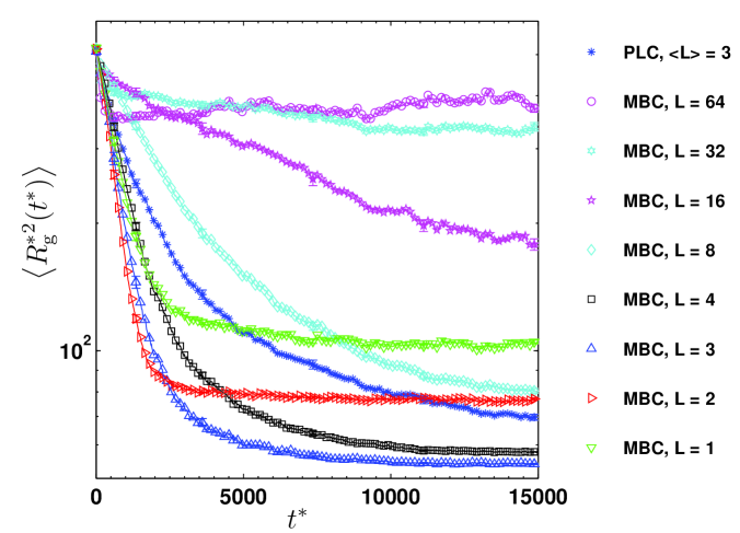
Figure 1: Variation of the mean square radius of gyration with time for $N=128$ chains, in the presence of HI, for (a) the PLC chain and MBC chains with various values of block length $L$, and (b) all three types of copolymers with values of average block length $\left\langle{L}\right\rangle\leq 4$.

3.1 Chain size

Figure 1 shows the effects of the block length $L$ for the protein-like, regular multi-block and random block copolymer chains on the evolution of the mean square radius of gyration for $N=128$, in the presence of HI. Obviously, the average block length plays an important role in controlling the dynamics of the process as well as the final equilibrium size of the copolymer chains. For the PLC chains in our model, the average block length $\left\langle{L}\right\rangle$, for both $N=64$ and $N=128$ bead chains, is approximately 3, which is very close to the value reported for the analogous lattice model ${}^{\hbox{\immediate{?},\penalty 1000{?}}}$ ($\left\langle{L}\right\rangle=3.173$).

We first discuss the effect of block length on the behaviour of the MBC chain. The simplest type of MBC is the diblock copolymer with $L=N/2$. It can be seen from Fig. 1 (a) that this diblock chain collapses to its equilibrium state faster than any of the other copolymer chains present in the plot. This is always true for such a copolymer because one of its ends (i. e. the end with the H block) behaves like a homopolymer chain in a poor solvent, which rapidly folds into its final equilibrium globular state, while the other end behaves like a homopolymer in a good solvent, remaining as a swollen coil. Due to the large size of this swollen part, the chain cannot form a compact equilibrium structure and consequently always has a relatively large final equilibrium size.

By reducing the block size to $L=32$, such that one has 4 blocks, one can see two time regimes of collapse. The first regime represents the early stage of collapse, where each H block of size $L$ rapidly folds into a single cluster. Thus at the end of this stage, the chain consists of $N/(2L)$ clusters or pearls separated by strings of P block chains. Since the folding of the H block is entirely homopolymer-like and is unaffected by the P type monomers, the time taken for each of these H block chains to completely fold into a small cluster is quite small, and it becomes systematically smaller for decreasing block size, such that it becomes hardly observable for shorter blocks.

The second regime represents the growth or coalescence of these intrachain clusters into a single large cluster. These clusters are separated from each other by a string of P block, which has the same size as that of the original H block. If the separation between the two intrachain clusters is larger than the range of the attractive interaction (or, equivalently, if the P block length is large enough), then these intrachain clusters go through a diffusion-like process. It is only when they interact with each other, i. e. when their separation distance comes within the range of attractive interaction, that they coalesce. Thus the growth of the average cluster size is quite gradual in this case. However, if the P block chain length is sufficiently small, such that two intrachain clusters are within the range of their attractive interaction, then the two clusters quickly coalesce to form a larger cluster and diffusion plays little or no role. Moreover, the average cluster size will also grow much more rapidly, or, equivalently, there is a rapid reduction in chain size. Since the diffusion time increases with the size of the intervening P block ,${}^{\hbox{\immediate{?}}}$ it is expected that the coalescence time is shorter for smaller P block sizes and consequently the collapse is much more rapid compared to large P block sizes. Furthermore, a large P block size leads to a less compact final collapsed size because blocks of P beads are always repelled from the core of H beads, and they form dangling legs extruding away from the core. The results for $L=32$ to $L=8$ for MBC chains in Fig. 1 (a) also confirm these expectations.

Note that for all MBC chains with $L\geq 8$, the final equilibrium size is still larger than that of the PLC chain. However, when $L=4$, the MBC chain reaches its equilibrium native state faster, and the final equilibrium size is smaller than that of a PLC chain. Reducing the block size of the MBC chain to $L=3$ further reduces the final size as well as the total collapse time. In fact, the data shows that the MBC chain with $L=3$ produces the lowest final equilibrium size compared to all other types of copolymer chains for the entire range of $L$ and $\left\langle{L}\right\rangle$ values that have been investigated. The total collapse time and the mean square radius of gyration for all three types of copolymers are listed in Table 1.

Type	$\left\langle{L}\right\rangle$	$\alpha$	$z$	$\tau$	$\left\langle{R_{\text{g}}^{2}}\right\rangle_{\text{eq}}$
PLC	3	0.945 $\pm$ 0.021	0.510 $\pm$ 0.009	5732 $\pm$ 146	69.762 $\pm$ 1.151
MBC	64	0.999 $\pm$ 0.012	0.920 $\pm$ 0.044	2044 $\pm$ 185	369.034 $\pm$ 8.605
MBC	32	0.978 $\pm$ 0.022	0.158 $\pm$ 0.003	N/A	N/A
MBC	16	0.842 $\pm$ 0.043	0.441 $\pm$ 0.005	N/A	N/A
MBC	8	0.616 $\pm$ 0.020	0.646 $\pm$ 0.004	6670 $\pm$ 139	79.819 $\pm$ 0.989
MBC	4	1.033 $\pm$ 0.026	0.819 $\pm$ 0.017	4248 $\pm$ 101	57.616 $\pm$ 0.064
MBC	3	1.316 $\pm$ 0.088	0.858 $\pm$ 0.018	3304 $\pm$ 118	54.287 $\pm$ 0.239
MBC	2	1.287 $\pm$ 0.029	1.008 $\pm$ 0.025	1967 $\pm$ 53	77.051 $\pm$ 0.385
MBC	1	0.929 $\pm$ 0.038	0.857 $\pm$ 0.018	2771 $\pm$ 103	103.906 $\pm$ 1.134
RBC	4	0.987 $\pm$ 0.028	0.631 $\pm$ 0.008	5447 $\pm$ 138	71.511 $\pm$ 1.278
RBC	3	1.071 $\pm$ 0.025	0.575 $\pm$ 0.006	5496 $\pm$ 141	64.513 $\pm$ 1.006
RBC	2	1.045 $\pm$ 0.037	0.595 $\pm$ 0.009	4948 $\pm$ 132	62.839 $\pm$ 0.985

Table 1: Values of the exponents for the early stages of collapse and the growth of the number average cluster size (i. e. $\alpha$ and $z$ in $\left\langle{R^{2}_{\text{g}}(0)}\right\rangle-\left\langle{R^{2}_{\text{g}}(t)}\right\rangle\sim t^{\alpha}$ and $\left\langle{S_{n}}\right\rangle\sim t^{z}$) for all types of copolymers with $N=128$ at various values of average block lengths $\left\langle{L}\right\rangle$, in the presence of HI. Values of the total collapse time $\tau$ and the equilibrium mean square radius of gyration $\left\langle{R^{2}_{\text{g}}}\right\rangle_{\text{eq}}$ are listed as well. Note that PLC, MBC and RBC denote protein-like, multi-block and random-block copolymers, respectively.

Further reduction in the block size to $L=2$ leads to a slightly faster collapse (as evidenced by the value of $\tau$ in Table 1), but it also increases the final chain equilibrium size. Note that for every $L$ monomers of H type that fuse with another H cluster, $L$ monomers of P type are brought into close proximity, due to the connectivity along the chain. As a result, a repulsive force builds up as the coalescence process takes place. For the $L=2$ chain, the energy gained from coalescence cannot overcome this repulsion, and therefore the chain does not form a single cluster of H monomers, i. e. it cannot fold into a spherical compact globule. The $L=1$ case conforms to this behaviour, with the chain collapsing slower, and the final equilibrium size being even larger than for $L=2$.

The large repulsive force built up due to the overcrowded presence of P type monomers for MBC chains with $L\leq 2$ can also be observed via the high value of the internal energy $U$ in Fig. 2. Note that the internal energy for MBC chains with $L=32$ and 16 is not reported here because the chains with these block sizes had not yet reached their equilibrium state, which is also subject to large fluctuations. This figure also clearly indicates that a chain which has the lowest equilibrium size does not necessarily have the lowest internal energy. Moreover, a chain with the lowest internal energy may not fold into the most compact final structure. This finding is consistent with the results of Ref. ?, where BD simulations without HI were performed.

Figure 2: Coordinate pairs ($U,\left\langle{{R_{\text{g}}^{*}}^{2}}\right\rangle_{\text{eq}}$) of the internal energy and $\left\langle{{R_{\text{g}}^{*}}^{2}}\right\rangle_{\text{eq}}$, respectively, in the final collapsed state for all copolymer chains with $N=128$, in the presence of HI.

From Fig. 1 (b), we can see that the PLC chain and the RBC chain with $\left\langle{L}\right\rangle=4$ are almost identical in terms of their final sizes and their time behaviour of $R_{\text{g}}$. However, reducing the average block size of the RBC chain to $\left\langle{L}\right\rangle=3$ and $\left\langle{L}\right\rangle=2$ systematically decreases both the collapse time and the equilibrium size even further. This finding is at variance with the results of Ref. ?, where the PLC chain was found to collapse more rapidly and into a more compact structure than the RBC chain with the same $\left\langle{L}\right\rangle$. It is not quite clear what the origin of this discrepancy is; most likely it is the fact that our model is a bead–spring model in the continuum, while Ref. ? studied a lattice model, which results in different local packing geometries, which are certainly very important for this problem. Another possible source could be different interaction parameters. The fact that we study a system with HI and Ref. ? one without can however not be used as an explanation; as Fig. 3 shows, we find the same behaviour also in the absence of HI (see below). For the protein folding problem this result indicates that the relation between the sequence and the thus-encoded collapse kinetics and native state is probably more intricate than the simple and appealing picture that the labeling procedure of Ref. ? suggests.

Figure 3: Variation of the mean square radius of gyration with time for all three types of copolymer chains with $N=128$, for various values of the average block length $\left\langle{L}\right\rangle$, in the absence of HI.

We fitted a power law

$$\left\langle{R^{2}_{\text{g}}(t)}\right\rangle=\left\langle{R^{2}_{\text{g}}(0)}\right\rangle-At^{\alpha}$$ (15)

to the initial decay of the mean square gyration radius, and the resulting exponents $\alpha$ are listed in Table 1. For a homopolymer chain at the same quench depth, Ref. ? had obtained a value of $\alpha=1.05\pm 0.01$ in the presence of HI. Interestingly, it can be seen from Table 1 that there exist some copolymer chains which have a larger exponent for this early stage compared to that of a homopolymer chain. Similar results have also been observed in Ref. ? for copolymer chains in the absence of HI.

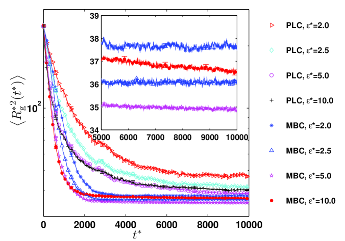
Figure 4: Variation of the mean square radius of gyration with time for chains with $N=64$, in the presence of HI, for (a) PLC and MBC chains with block length of $L=3$, and (b) PLC and RBC chains with an average block length of $\left\langle{L}\right\rangle=3$. Here, $\epsilon^{*}$ denotes the value of the quench depth or $\epsilon_{\text{LJ}}/k_{\text{B}}T$. Insets: Variation of the mean square radius of gyration with time for chains with $N=64$ and $L=3$ or $\left\langle{L}\right\rangle=3$ at various quench depths $\epsilon^{*}$, for (a) MBC chain, and (b) PLC chain.

3.2 Influence of HI

In order to study the influence of HI, we have also carried out simulations without HI, for the case $N=128$, and the results are shown in Fig. 3. We find that in general the collapse dynamics is substantially slowed down, compared to the HI case, which corresponds to the observation for homopolymers that the presence of HI (Zimm model) leads to systematically faster dynamics than in the case when HI is absent (Rouse model). In most cases, the chains had not even relaxed fully into equilibrium at the time at which the HI runs (and also the non-HI runs) were stopped. For the one case in which equilibrium was reached, we find the same value for $\left<R_{\text{g}}^{2}\right>_{\text{eq}}$ as in the case with HI, as it must be. The qualitative results concerning the influence of the chain architecture on the collapse kinetics remain however completely unchanged: Again, the PLC chain corresponds to the $\left\langle{L}\right\rangle=4$ RBC, but the RBCs with shorter block length collapse even faster.

The observed acceleration of the collapse dynamics as a result of HI is consistent with our previous findings on homopolymer collapse ,${}^{\hbox{\immediate{?}}}$ where it was shown that for $N=128$ the inclusion of HI reduces the total collapse time by at least a factor of two. A complete comparison between the total collapse times for cases with and without HI is not reported in this work, due to the slow convergence to equilibrium in the absence of HI. The only case where equilibrium was reached (MBC, $L=2$) seems to indicate that the speedup is even larger in the present case ($\tau=5233$ without HI, $\tau=1967$ with HI). Since hydrodynamics is a large-scale phenomenon, one expects the effect of HI to be the more dramatic the more extended the objects are. Due to the uncollapsed P strings, the chains stay systematically longer in an extended state than in the homopolymer case, and this is probably the reason why HI has an even stronger effect.

3.3 Influence of quench depth

We have simulated $N=64$ chains at various values of the quench depth $\epsilon^{*}$, in order to study the influence of this parameter, while keeping the block length (or average block length) at $L=3$ (or $\left\langle{L}\right\rangle=3$). Figure 4 shows the results for the gyration radius. For all the quench depths investigated, it can be seen that the MBC chains collapse the fastest and have the most compact equilibrium size, followed by the RBC chains. Out of all three types of copolymer chains, the PLC chain collapses the slowest and the final equilibrium size is the least compact. Generally, one would expect that the radius of gyration for a chain at deep quench should be smaller than that of a chain with lower quench values because the stronger attractive interaction would cause the chain to squeeze into a tighter globule. The above figure shows that a chain smoothly folds into its final compact state for low quench depth. However, at very large quench depth (i. e. $\epsilon_{\text{LJ}}/k_{\text{B}}T=10$), a chain gets trapped in a metastable state and stays there for a long time rather than approach its final minimum energy state. The inset of Fig. 4 (a) shows this trapping behaviour at very large quench depths much more clearly for an MBC chain. This inset reveals that, while MBC chains with $\epsilon_{\text{LJ}}/k_{\text{B}}T\leq 5$ have fully reached their equilibrium compact state, chains with $\epsilon_{\text{LJ}}/k_{\text{B}}T=10$ are still gradually approaching the equilibrium state. A similar result is also observed for other types of copolymer chains (see Fig. 4 (b)). A similar behaviour has been observed by various other authors .${}^{\hbox{\immediate{?},\penalty 1000{?},\penalty 1000{?},\penalty 1000{\bf{?}}}}$ In Ref. ? it was found that a homopolymer chain will get trapped at $\epsilon_{\text{LJ}}/k_{\text{B}}T=5$, while our results indicate that a copolymer chain still smoothly folds at this quench depth. This result seems to indicate that the presence of P type monomers in the chain prevents it from being trapped in a local well and smooths out the energy landscape for the folding process of copolymers. This in turn pushes the value of quench depth where trapping occurs to a much higher value.

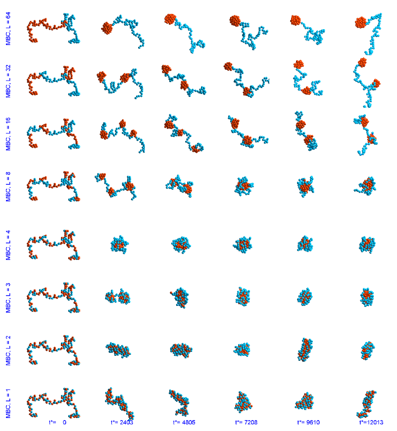
Figure 5: Snapshots of different types of collapsing regular multi-block copolymers (MBC) chain with $N=128$, in the presence of HI.

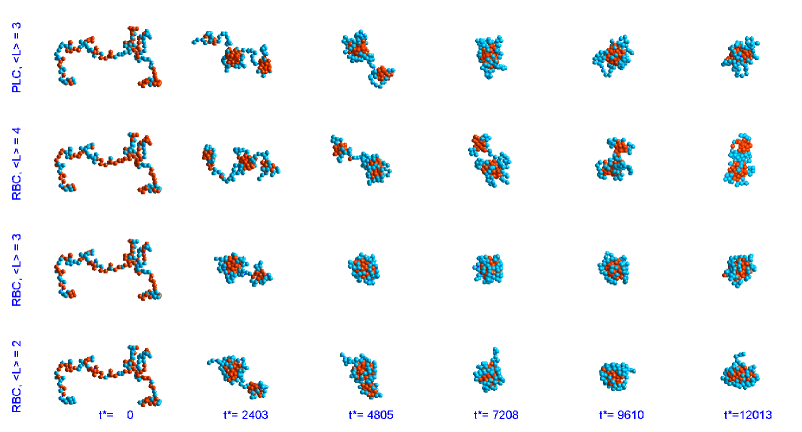
Figure 6: Snapshots of different types of collapsing protein-like copolymers (PLC) and random-block copolymers (RBC) chains with $N=128$, in the presence of HI.

Figure 7: Variation of the ratio of the largest eigenvalue to the smallest eigenvalue of the gyration tensor with time for all three types of copolymer chains with $N=128$, for various values of the average block length $\left\langle{L}\right\rangle$, in the presence of HI. Inset: The corresponding variation of the smallest eigenvalue with time. Here, the symbol $\lambda_{i}$ is actually an abbreviation for $\left\langle{\lambda_{i}^{2}}\right\rangle^{1/2}$.

3.4 Snapshots

Snapshots of the typical kinetic pathways for a collapsing chain of length $N=128$ for MBC chains are shown in Fig. 5, and for PLC and RBC chains in Fig. 6. For some selected cases, we show the time evolution in the movie files S1.avi and S2.avi of the Supporting Information. It can be seen that there exist at least two distinct stages for the kinetics of collapse for these copolymers. It is to be noted that almost all of the copolymer chains with sequences that fold into a spherical compact structure have a three-stage mechanism. The early stage involves the rapid formation of localised globules along the chain. Following this stage, these globules then coalesce together by fusing with other nearby blobs to form a dumbbell or two pearls separated by linear chain. Finally, the pearls combine to form a sausage which slowly rearranges itself into a compact state. However, for copolymer chains with sequences consisting of short P blocks that do not fold into a spherical compact structure (for instance, MBC chains with $L\leq 2$), only the first two distinct stages are observed and the final compaction stage apparently does not occur. Furthermore, copolymer chains with sequences consisting of large P blocks, such as MBC chains with $L=32$ and 16, seem to acquire another distinct stage after the early rapid collapse stage, known as the “diffusion” or “plateau” regime. During this diffusion stage, the number and size of the intrachain clusters remains unchanged due to the large separation between the H blocks. Similar qualitative features of the collapse pathways have also been observed by other authors .${}^{\hbox{\immediate{?},\penalty 1000{\bf{?}}}}$

3.5 Asphericity

Apart from the snapshots, the asphericity of the chain can also be observed from the eigenvalues of the gyration tensor. Figure 7 shows the time evolution of the ratio of the largest eigenvalue to the smallest eigenvalue for all three types of copolymer chains with $N=128$, for various values of the average block length $\left\langle{L}\right\rangle$, in the presence of HI. Interestingly, the data in Fig. 7 clearly shows that this ratio of eigenvalues behaves non-monotonically with time. A similar result is also observed for the ratio of the intermediate eigenvalue to the smallest eigenvalue $\lambda_{2}/\lambda_{3}$. The non-monotonic behaviour is mainly due to the non-monotonic nature of the smallest eigenvalue $\lambda_{3}$, as can be seen in the inset of Fig. 7. This behaviour can be explained by the fact that during the collapse of the chain, there is a sudden change in the shape of the chain from an initial “ellipsoid” (note that a typical self-avoiding walk is highly anisotropic) to a pearl-necklace and finally (typically) to a sphere. During this shape transformation, the eigenvalue for the smallest principal axis is first reduced to the lowest value, at which the thinnest pearl-necklace chain is formed. This principal axis then grows in width when the pearl-necklace chain starts to transform by absorbing nearby pearls or clusters, and when the bridging strings of monomers form a final spherical structure. Note that a similar result has also been observed for a homopolymer chain .${}^{\hbox{\immediate{?}}}$

Figure 8: Variation of the number average cluster size with time for chains with $N=128$ in the presence of HI, for (a) MBC chains, (b) the PLC chain and RBC chains with $\left\langle{L}\right\rangle\leq 4$, and (c) MBC chains with $L=32$ and 16.

Figure 9: Variation of the number of clusters with time for the PLC and MBC chains, in the presence of HI.

Figure 10: Coordinate pairs ($L_{\text{P}},z$) of the block size of P type monomers and the coarsening stage exponent, respectively, for MBC chains and a homopolymer chain with $N=128$, in the presence of HI.

3.6 Cluster analysis

The growth of the number average cluster size with time for our chosen value of overlapping distance $D^{*}=1.2\times 2^{1/6}(\sigma/l_{H})$ is shown in Fig. 8. The most striking aspect about these data is their quantitative demonstration of the multi-stage process of collapse kinetics, already indicated qualitatively by inspection of snapshots, in a much clearer fashion than by the data on the gyration radius. Typically, there are three growth regimes: (i) Collapse of the single H blocks on a fairly short time scale, giving rise to a moderate increase in the mean cluster size $\left\langle{S_{n}}\right\rangle$; (ii) Coalescence of these clusters at a later time scale, resulting in a steep increase in cluster size; and finally (iii) internal rearrangement of the resulting “sausage” that does not change $\left\langle{S_{n}}\right\rangle$ anymore. However, for MBC chains with large block size (i. e. $L=32$ and 16, see Fig. 8 (c)) yet another (fourth) regime can be observed, which follows directly the initial single-block collapse, and which is characterised by a constant value of $\left\langle{S_{n}}\right\rangle$. This clearly corresponds to the time regime that is needed for the single globules to find each other in a diffusion-like process.

This diffusion regime for MBC chains with large P blocks is also observed in the time evolution of the number of clusters $N_{\text{c}}$, as shown in Fig. 9: While the $L=64$ chain (diblock copolymer) shows a simple decay of $N_{\text{c}}$ to $N_{\text{c}}=1$, i. e. coalescence of smaller clusters to one large globule, the chains with more blocks ($L=32,16,8$) exhibit a clear plateau at $N_{\text{c}}=N/(2L)$, i. e. the number of H blocks. For smaller block sizes, such a plateau is no longer clearly identifiable, since the intervening P blocks are too short to keep the H clusters away from each other. Interestingly, for $L=2$, $N_{\text{c}}$ exhibits a clear maximum, which corresponds to breakup and coalescence of clusters. Furthermore, the PLC chain, whose data is shown for comparison, shows just a smooth decay to $N_{\text{c}}=1$, without any visible structure.

During the cluster coalescence stage, previous studies of homopolymer chains indicate that one might expect a power law

$$\left\langle{S_{n}(t)}\right\rangle\sim t^{z}.$$ (16)

We therefore fitted such a behaviour to our data; the results for the exponent $z$ are listed in Table 1. Interestingly, the $z$ values that we find for our copolymers are always smaller than the value $z=1.08\pm 0.01$ obtained for a homopolymer .${}^{\hbox{\immediate{?}}}$ Given the fact that the obtained values differ from each other substantially, it is far from clear that the obtained numbers have much to do with a well-defined asymptotic power law. Furthermore, the fact that the coalescence process involves two competing length scales (the average globule size of the consolidated clusters, and the size of the P “loops”) makes the application of self-similarity arguments, which are usually employed in order to justify power-law behaviour, rather doubtful. On the other hand, the fact that the $z$ value depends systematically on the block length (as shown in Fig. 10 for the homopolymer and MBC chains up to block length $L=32$) makes the interpretation of $z$ in terms of an effective exponent, which in reality describes a more complicated dynamics, fairly likely.

Noticeably, data for MBC chains with $L=1$ and $L=2$ in Fig. 10 do not lie on the smooth curve that can be drawn by eye through all the remaining chains starting from the homopolymer chain to the MBC chain with $L=32$. As discussed earlier, for these two MBC chains, repulsive forces build up during the coalescence process due to the close proximity of the P blocks with each other. This leads to an equilibrium state with the highest energy (Fig. 2), and the highest asphericity, as evident from the snapshot (Fig. 5), and the ratio of the largest to smallest eigenvalue (Fig. 7). The non-occurrence of the final cluster consolidation stage into a compact globule as a consequence of the built up repulsive energy is probably the reason for the data for these two chains not following the general trend seen in the case of the other MBC chains. A similar pattern is seen below in the correlation between the collapse time and block size, and equilibrium mean square gyration radius.

Figure 11: Coordinate pairs ($L_{\text{P}},\tau$) of the block size of P type monomers and total collapse time for MBC chains and a homopolymer chain with $N=128$, in the presence of HI.

Figure 12: Total collapse time versus equilibrium mean square gyration radius for $N=128$ copolymer chains of different types, in the presence of HI.

3.7 Collapse time

The characteristic collapse times $(\tau)$ for all three types of copolymers with $N=128$ are shown in Table 1. It is observed that for all types of copolymers used in this work, the collapse time is much larger than the collapse time for a homopolymer chain, for which $\tau=591\pm 7$. As has been pointed out earlier, MBC chains with $L=32$ and 16 had not yet reached their equilibrium state during the course of our simulation, and hence the total collapse time for these two chains are not available. The collapse time also increases systematically with the block size, as demonstrated in Fig. 11 for the homopolymer and MBC chains up to $L=8$. These data hence clearly indicate that the block size of P monomers not only controls the duration of the diffusion process, but also the collapse rate of the cluster coalescence stage for copolymers with small P block size where diffusion plays little or no role. The combined diffusion and cluster consolidation process is thus identified as the decisive rate-limiting factor for the overall collapse. The absence of these processes for a homopolymer leads to a much faster collapse, and also leads in the case of MBC chains with $L=1$ and $L=2$, to a departure from the observed trend for the other chains.

In order to understand the relationship between the kinetic accessibility of the final state and the final equilibrium size, we plot the collapse time versus the final size in Fig. 12. Except for MBC chains with $L=1$ and $L=2$ (for the reasons discussed earlier), the figure clearly demonstrates that the total collapse time is directly related to the final equilibrium size. This result reveals a very interesting feature that is somewhat unexpected, i. e., a chain with a small equilibrium size tends to fold much more rapidly than a chain with a larger equilibrium size. Intuitively, one might expect that it would take longer for a chain to fold into a more compact equilibrium structure rather than into a loosely packed structure, but the present results suggest the opposite. In Ref. ? it was pointed out that a pronounced energy minimum is a necessary condition to guarantee that the native state is stable, and that such a minimum is sufficient, for a compact globule with random structures, to rapidly find the native state. Thus the deep energy minimum of the compact structure seems to provide a guide (or a strong thermodynamic driving force) for the chain to quickly fold into its final equilibrium state. In the present work, we have made no attempts to determine the free energy of the chains. However, we anticipate that knowledge of the relationship between the free energy of the native state and the size of the native conformation may help in understanding this behaviour better.

3.8 Block size distribution

Figure 13: The tails of the normalised distribution of P blocks for a protein-like copolymer (PLC) and random-block copolymers (RBC) with three different average block lengths $\left\langle{L}\right\rangle$, for $N=128$. Inset: The complete normalised distribution for PLC and RBC chains.

As has been discussed above, the length of P blocks for MBC chains has a very decisive influence on the kinetics (large blocks lead to a substantial slowing down of the process) as well as on the equilibrium size (large blocks increase the size). Since this influence is very strong, one might expect that in disordered copolymers the presence of such large blocks should also have a substantial influence, even if their probability of occurrence is fairly small. We have therefore analysed the probability distribution of P block lengths for the PLC chains that we have generated, and compare it in Fig. 13 to the Poisson distributions of RBC chains with similar $\left\langle{L}\right\rangle$. The inset shows the total distributions, but for our purposes the tails of the distributions at large $L$ values are of particular interest; hence they are shown in the main part. We find the very interesting result that for the PLC chains the tail is substantially enhanced compared to the Poissonians with $2\leq\left\langle{L}\right\rangle\leq 4$. It is therefore quite natural to assume that it is this enhanced tail that leads to the slowed-down dynamics of the PLC, compared to the RBC with identical $\left\langle{L}\right\rangle$. If this correlation is really valid, then one should expect that the lattice PLC chains of Ref. ? should show a deflated tail, in comparison to the corresponding RBCs, as a result of different packing behaviour. It should be quite interesting to test this.

4 Summary and conclusions

We have shown that Brownian Dynamics simulations incorporating implicit hydrodynamic interactions can be used to study the dynamics of copolymer collapse in a poor solvent. Our observations regarding the speedup of collapse caused by hydrodynamic interactions, and the existence of at least two stages of collapse, are similar to those that have been reported previously in the literature. Due to the inherent computational advantages of an implicit-solvent model, compared to, say, straightforward Molecular Dynamics with explicit solvent, we were able to study the phenomena with reasonable statistical accuracy.

The kinetics of collapse can be described as a rapid initial formation of clusters followed by cluster coalescence and sometimes a rearrangement of the final cluster to form a compact state. It is also found that the presence of P monomers pushes the value of quench depth at which trapping phenomena occur to a higher value compared to the value seen for homopolymer chains. A striking feature observed here is that the total collapse time is completely governed by the cluster consolidation stage and the rate of collapse of this stage depends on the block size of P monomers along the chain. It is found that in our model random block copolymers collapse more rapidly than “protein–like” copolymers with the same average block length, if the latter are generated by the labelling procedure suggested in Ref. ?, and this behaviour can apparently be traced back to an enhanced occurrence of long P blocks in the PLCs.

We finally emphasise again that our model is intended as a “toy model” designed to study the influence of certain aspects (monomer sequence, hydrodynamic interactions) on the collapse kinetics, which cannot be expected to be directly related to real proteins. To illustrate this point, let us assume that each model monomer corresponds to a single amino acid residue, with a typical size of, say, $1nm$, which would then be the value of $l_{H}$ in real units. Since we are only interested in order–of–magnitude estimates here, this could also be taken as the value for $\sigma$ or for $Q_{0}$. A chain of $N=64$ or $128$ would then correspond to a fairly short polypeptide whose native state would typically need to be described in terms of a much more elaborate geometry (e. g. alpha helices, beta sheets) than just a spherical or sausage–like globule. The elementary time scale $\lambda_{H}$ is then found via

$$\lambda_{H}=\frac{\zeta}{4H}=6\pi\eta_{s}a\frac{l_{H}^{2}}{4k_{B}T},$$ (17)

where $a$, the Stokes radius of the model monomer, is given by

$$a=h^{\star}\sqrt{\pi}l_{H},$$ (18)

such that we find

$$\lambda_{H}=\frac{3}{2}\sqrt{\pi}h^{\star}\frac{\eta_{s}l_{H}^{3}}{k_{B}T}.$$ (19)

For our value of $h^{\star}$, and assuming the viscosity of water and room temperature, we thus find $\lambda_{H}\approx 0.3ns$ as our elementary time unit. A collapse time of $6000$ in our BD units would thus correspond to roughly $2\mu s$. This value should however not be taken too seriously, since our model does not include bond–bending and torsional potentials and other interactions that would be needed to describe the structure and energetics on such a small length scale. Furthermore, the value of $l_{H}$, which we have essentially just guessed, enters with the third power. Nevertheless, it may be noted that detailed simulations and experiments on real proteins ${}^{\hbox{\immediate{\bf{?}}}}$ have also produced collapse times in the microsecond range, whose values are however somewhat larger, for chains that are even shorter. In general, we believe that the simplicity of our model results in a lack of local kinetic barriers, such that our estimate for the collapse time tends to be smaller than the folding time of the “corresponding” real protein. In this context, it should also be noted that the interpretation of one model monomer in terms of just one residue is certainly not imperative. One could as well consider a model where one model monomer corresponds to several residues (under the assumption that proteins with such long blocks exist). In this case, one would have a larger value for $l_{H}$, and therefore a very much larger folding time in real units.

References and Notes

- (1) Nishio, I.; Sun, S. T.; Swislow, G.; Tanaka, T. Nature 1979, 281, 208–209.
- (2) de Gennes, P.-G. Scaling concepts in polymer physics; Cornell University Press: Ithaca, 1979.
- (3) de Gennes, P.-G. Phys. Rev. Lett. 1985, 46, 639 - 642.
- (4) Buguin, A.; Wyart, F. B.; deGennes, P. G. C. R. Acad. Sci., Ser. IIb: Mec., Phys., Chim., Astron. 1996, 322, 741-746.
- (5) Creigton, T. E. Protein Folding; Freeman: New York, 1994.
- (6) Frembgen-Kesner, T.; Elcock, A. H. J. Chem. Theo. Comp. 2009, 5, 242-256.
- (7) Cieplak, M.; Niewieczerzal, S. J. Chem. Phys. 2009, 130, 124906 (R).
- (8) Lifshitz, I. M.; Grosberg, A. Y.; Khokhlov, A. R. Rev. Mod. Phys. 1978, 50, 683-713.
- (9) Ostrovsky, B.; Baryam, Y. Europhys. Lett. 1997, 25, 409-414.
- (10) Kuznetsov, Y. A.; Timoshenko, E. G.; Dawson, K. A. J. Chem. Phys. 1995, 103, 4807-4818.
- (11) Tanaka, G.; Mattice, W. L. Macromolecules 1995, 28, 1049-1059.
- (12) Byrne, A.; Kiernan, P.; Green, D.; Dawson, K. A. J. Chem. Phys. 1995, 102, 573-577.
- (13) Grassberger, P. Phys. Rev. E 1997, 56, 3682-3693.
- (14) Klushin, L. I. J. Chem. Phys. 1998, 108, 7917-7920.
- (15) Halperin, A.; Goldbart, P. M. Phys. Rev. E 1999, 60, 2111-2124.
- (16) Polson, J. M.; Zuckermann, M. J. J. Chem. Phys. 2000, 113, 1283-1293.
- (17) Chang, R.; Yethiraj, A. J. Chem. Phys. 2001, 114, 7688–7699.
- (18) Abrams, C. F.; Lee, N. K.; Obukhov, S. P. Europhys. Lett. 2002, 59, 391-397.
- (19) Polson, J. M.; Zuckermann, M. J. J. Chem. Phys. 2002, 116, 7244-7254.
- (20) Kikuchi, N.; Gent, A.; Yeomans, J. M. Eur. Phys. J. E 2002, 9, 63-66.
- (21) Kikuchi, N.; Ryder, J. F.; Pooley, C. M.; Yeomans, J. M. Phys. Rev. E 2005, 71, 61804 - 1.
- (22) Polson, J. M.; Moore, N. E. J. Chem. Phys. 2005, 122, 024905.
- (23) Lee, S. H.; Kapral, R. J. Chem. Phys. 2006, 124, 214901.
- (24) Pham, T. T.; Bajaj, M.; Prakash, J. R. Soft Matter 2008, 4, 1196-1207.
- (25) Hayes, B. American Scientist 1998, 86, 216-221.
- (26) Lau, K. F.; Dill, K. A. Macromolecules 1989, 22, 3986-3997.
- (27) Chan, H. S.; Dill, K. A. Proteins-Structure Function And Bioinformatics 1996, 24, 335-344.
- (28) Cooke, I. R.; Williams, D. R. M. Macromolecules 2003, 36, 2149-2157.
- (29) White, S. H.; Jacobs, R. E. J. Mol. Evol. 1993, 36, 79-95.
- (30) Dill, K. A. Biochemistry 1985, 24, 1501-1509.
- (31) Camacho, C. J.; Thirumalai, D. Phys. Rev. Lett. 1993, 71, 2505-2508.
- (32) Halperin, A. Macromolecules 1991, 24, 1418-1419.
- (33) Timoshenko, E. G.; Kuznetsov, Y. A.; Dawson, K. A. Phys. Rev. E 1996, 53, 3886-3899.
- (34) Villeneuve, C.; Guo, H.; Zuckermann, M. J. Macromolecules 1997, 30, 3066-3074.
- (35) Timoshenko, E. G.; Kuznetsov, Y. A.; Dawson, K. A. Phys. Rev. E 1998, 57, 6801-6814.
- (36) Khokhlov, A. R.; Khalatur, P. G. Physica A 1998, 249, 253-261.
- (37) Khokhlov, A. R.; Khalatur, P. G. Phys. Rev. Lett. 1999, 82, 3456-3459.
- (38) Ganazzoli, F. J. Chem. Phys. 2000, 112, 1547-1553.
- (39) Shakhnovich, E. I.; Gutin, A. M. Protein Engineering 1993, 6, 793-800.
- (40) Shakhnovich, E. I.; Gutin, A. M. Proc. Natl. Acad. Sci. USA 1993, 90, 7195-7199.
- (41) Shakhnovich, E. I. Phys. Rev. Lett. 1994, 72, 3907-3910.
- (42) Öttinger, H. C. Stochastic Processes in Polymeric Fluids; Springer: Berlin, 1996.
- (43) Prabhakar, R.; Prakash, J. R. J. Non-Newtonian Fluid Mech. 2004, 116, 163–182.
- (44) Sunthar, P.; Prakash, J. R. Macromolecules 2005, 38, 617-640.
- (45) Rotne, J.; Prager, S. J. Chem. Phys. 1969, 50, 4831–4837.
- (46) Yamakawa, H. Modern Theory of Polymer Solutions; Harper and Row: New York, 1971.
- (47) Prabhakar, R.; Prakash, J. R.; Sridhar, T. J. Rheol. 2004, 48, 1251–1278.
- (48) Sevick, E. M.; Monson, P. A.; Ottino, J. M. J. Chem. Phys. 1988, 88, 1198 - 1206.
- (49) Ziv, G.; Thirumalai, D.; Haran, G. Phys. Chem. Chem. Phys. 2009, 11, 83-93.
- (50) Dasmahapatra, A. K.; Kumaraswamy, G.; Nanavati, H. Macromolecules 2006, 39, 9621-9629.
- (51) Sali, A.; Shakhnovich, E.; Karplus, M. Nature 1994, 369, 248-251.
- (52) Snow, C.; Nguyen, H.; Pande, V.; Gruebele, M. Nature 2002, 420, 102–106.