Abstract

In the $SO(5)\times U(1)$ gauge-Higgs unification model in the Randall-Sundrum warped space there results the conservation of the $H$ parity. The $H$ parity is assigned to all 4D fields including excited modes in Kaluza-Klein towers. The neutral Higgs boson is the lightest particle of odd $H$ parity, consequently becoming absolutely stable. Its mass is found to be $70\sim 135\,$GeV for the warp factor $z_{L}=10^{5}\sim 10^{15}$.

1 Introduction

The Higgs boson is the only particle yet to be found in the standard model of electroweak interactions. It is not clear, however, if the Higgs boson appears as described in the standard model (SM). New physics may be hidden behind it.

One possible scenario is gauge-Higgs unification, in which spacetime has more than four dimensions and electroweak gauge symmetry is broken by quantum dynamics in the extra dimension.[2, 3, 4] The 4D Higgs boson, which becomes a part of gauge fields, appears as an Aharonov-Bohm (AB) phase in a non-simply-connected extra dimension. Its finite mass $m_{H}$ is generated at the quantum level. A non-vanishing AB phase $\theta_{H}$, or the Higgs vev, induces electroweak symmetry breaking and gives masses to quarks, leptons, $W$ and $Z$.[5]-[36]

In the $SO(5)\times U(1)$ gauge-Higgs unification model it has been shown that the value $\theta_{H}=\hbox{${1\over 2}$}\pi$ is dynamically chosen,[27] and the 4D Higgs boson becomes stable.[29] It has been shown that a new parity, $H$ parity, appears among low energy particles. Only the Higgs boson is $H$ parity odd, while all other particles in the standard model are $H$ parity even. The stability implies that Higgs bosons become dark matter of the universe. The relic density of cold dark matter observed at WMAP can be obtained with $m_{H}\sim 70\,$GeV.

The gauge-Higgs unification scenario leads to many phenomenological consequences. The nature of the Higgs boson as an AB phase leads to the stability against quantum corrections which gives a solution to the gauge-hierarchy problem.[5] Gauge-couplings of quarks and leptons slightly deviate from those in SM, whereas significant deviation appears in the Higgs couplings.[19, 28, 32] Distinctive prediction for anomalous magnetic moment and electric dipole moment has been discussed.[20, 24, 31] The spectrum and couplings of Kaluza-Klein (KK) excited states may differ from those in other extra-dimensional theories such as UED models.

In this paper we focus on the Higgs boson in the gauge-Higgs unification. As mentioned above, the Higgs boson becomes stable in a class of the $SO(5)\times U(1)$ gauge-Higgs unification models as a result of the $H$ parity conservation. In this regards we note that stable, or almost stable, Higgs bosons have appeared in other models. The inert doublet Higgs model of Deshpande and Ma is among them, in which a second Higgs field is introduced in addition to the standard Higgs field giving masses to quarks, leptons, $W$ and $Z$.[37] The model has a $Z_{2}$ symmetry such that the second Higgs field is odd, while other low energy fields are even. Because of this new $Z_{2}$ symmetry, or parity, the lightest Higgs boson of odd parity becomes stable. Many implications to dark matter and neutrino physics have been discussed.[38]-[46] Similarly the inert triplet Higgs model also serves as a minimal dark matter model.[47]-[49]

Although there is similarity in the Higgs boson between the inert Higgs models and the gauge-Higgs unification, there is crucial difference. In the $SO(5)\times U(1)$ gauge-Higgs unification there is only one Higgs doublet which is responsible for symmetry breaking and mass generation, and at the same time becomes absolutely stable. The $Z_{2}$ parity in the inert Higgs model is introduced by hand, whereas the $H$ parity in the gauge-Higgs unification is hidden in the original minimal model. It dynamically emerges as a result of the fact that the AB phase $\theta_{H}=\hbox{${1\over 2}$}\pi$ is realized in the vacuum.

Dynamically emergent $H$ parity plays a key role for the stability of the Higgs boson. Previously $H$ parity has been assigned only for low energy fields in the $SO(5)\times U(1)$ gauge-Higgs unification model. In this paper we show that the $H$ parity is assigned to all 4D fields. The selection rule associated with the $H$ parity conservation is useful in analyzing production of KK excited states, higher order corrections, and so on.

The organization of the paper is the following. In the next section the $SO(5)\times U(1)$ gauge-Higgs unification model is given and specified. In Section 3 we explain how parameters of the model relevant for low energy physics are determined. In Section 4 the effective potential $V_{\rm eff}(\theta_{H})$ is re-evaluated, and $m_{H}$ is determined as a function of the warp factor $z_{L}$. In Section 5 a proof is given for the enhanced gauge invariance which in turn implies that physics is periodic in $\theta_{H}$ with a period $\pi$ in the model. In Section 6 we show how the $H$ parity is assigned to all 4D fields. It is shown that the action including brane interactions is invariant under $H$ parity. A summary is given in Section 7.

2 Model

The $SO(5)\times U(1)$ scheme was first proposed by Agashe, Contino, and Pomarol,[13] and has been elaborated since then. The current model is given in ref.  [27] and elaborated to incorporate leptons in ref. [32]. It is defined in the Randall-Sundrum (RS) warped spacetime with a metric

$$ds^{2}=G_{MN}dx^{M}dx^{N}=e^{-2\sigma(y)}\eta_{\mu\nu}dx^{\mu}dx^{\nu}+dy^{2},\qquad$$ (2.1)

where $\eta_{\mu\nu}=\textrm{diag}(-1,1,1,1)$, $\sigma(y)=\sigma(y+2L)=\sigma(-y)$, and $\sigma(y)=k|y|$ for $|y|\leq L$. The Planck and TeV branes are located at $y=0$ and $y=L$, respectively. The bulk region $0<y<L$ is anti-de Sitter (AdS) spacetime with a cosmological constant $\Lambda=-6k^{2}$. The warp factor $z_{L}\equiv e^{kL}\gg 1$ plays an important role in subsequent discussions. The Kaluza-Klein (KK) mass scale is given by

$$m_{\rm KK}=\frac{\pi k}{z_{L}-1}\sim\pi kz_{L}^{-1}~{}.$$ (2.2)

The model consists of $SO(5)\times U(1)_{X}$ gauge fields $(A_{M},B_{M})$, bulk fermions $\Psi_{a}$, brane fermions $\hat{\chi}_{\alpha R}$, and brane scalar $\Phi$. The action integral consists of the bulk and brane parts; $S=S_{\rm bulk}+S_{\rm brane}$. The bulk part is given by

$$\hskip-28.45274ptS_{\rm bulk}=\int d^{5}x\sqrt{-G}\bigg{[}-{\rm tr\,}\Big{(}{1\over 4}F^{(A)MN}F_{MN}^{(A)}+{1\over 2\xi}(f_{\textrm{\scriptsize gf}}^{(A)})^{2}+{\cal L}_{\textrm{\scriptsize gh}}^{(A)}\Big{)}$$ (2.3)

$$\hskip 14.22636pt-\Big{(}{1\over 4}F^{(B)MN}F_{MN}^{(B)}+{1\over 2\xi}(f_{\textrm{\scriptsize gf}}^{(B)})^{2}+{\cal L}_{\textrm{\scriptsize gh}}^{(B)}\Big{)}+\sum_{a}i\bar{\Psi}_{a}{\cal D}(c_{a})\Psi_{a}\bigg{]},$$ (2.4)

$$\hskip-28.45274pt{\cal D}(c_{a})=\Gamma^{A}{e_{A}}^{M}\big{(}\partial_{M}+{1\over 8}\omega_{MBC}[\Gamma^{B},\Gamma^{C}]-ig_{A}A_{M}-ig_{B}Q_{Xa}B_{M}\big{)}-c_{a}\sigma^{\prime}(y)~{}.$$ (2.5)

The gauge fixing and ghost terms are denoted as functionals with subscripts gf and gh, respectively. $F_{MN}^{(A)}=\partial_{M}A_{N}-\partial_{N}A_{M}-ig_{A}[A_{M},A_{N}]$ and $F_{MN}^{(B)}=\partial_{M}B_{N}-\partial_{N}B_{M}$. The $SO(5)$ gauge fields $A_{M}$ are decomposed as

$$A_{M}=\sum_{I=1}^{10}A^{I}_{M}T^{I}=\sum_{a_{L}=1}^{3}A^{a_{L}}_{M}T^{a_{L}}+\sum_{a_{R}=1}^{3}A^{a_{R}}_{M}T^{a_{R}}+\sum_{\hat{a}=1}^{4}A^{\hat{a}}_{M}T^{\hat{a}}~{},$$ (2.6)

where $T^{a_{L},a_{R}}$ ($a_{L},a_{R}=1,2,3$) and $T^{\hat{a}}$ ($\hat{a}=1,2,3,4$) are the generators of $SO(4)\simeq SU(2)_{L}\times SU(2)_{R}$ and $SO(5)/SO(4)$, respectively.

In the fermion part $\bar{\Psi}=i\Psi^{\dagger}\Gamma^{0}$ and $\Gamma^{\mu}$ matrices are given by

$$\Gamma^{\mu}=\begin{pmatrix}&\sigma^{\mu}\cr\bar{\sigma}^{\mu}&\end{pmatrix},\quad\Gamma^{5}=\begin{pmatrix}1&\cr&-1\end{pmatrix},\quad\sigma^{\mu}=(1,\vec{\sigma}),\quad\bar{\sigma}^{\mu}=(-1,\vec{\sigma}).$$ (2.7)

All of the bulk fermions are introduced in the vector (5) representation of $SO(5)$. The $c_{a}$ term in Eq. (2.5) gives a bulk kink mass, where $\sigma^{\prime}(y)=k\epsilon(y)$ is a periodic step function with a magnitude $k$. The dimensionless parameter $c_{a}$ plays an important role controlling profiles of fermion wave functions.

The orbifold boundary conditions at $y_{0}=0$ and $y_{1}=L$ are given by

$$\hskip-28.45274pt\begin{pmatrix}A_{\mu}\cr A_{y}\end{pmatrix}(x,y_{j}-y)=P_{j}\begin{pmatrix}A_{\mu}\cr-A_{y}\end{pmatrix}(x,y_{j}+y)P_{j}^{-1},$$ (2.8)

$$\hskip-28.45274pt\begin{pmatrix}B_{\mu}\cr B_{y}\end{pmatrix}(x,y_{j}-y)=\begin{pmatrix}B_{\mu}\cr-B_{y}\end{pmatrix}(x,y_{j}+y),$$ (2.9)

$$\hskip-28.45274pt\Psi_{a}(x,y_{j}-y)=P_{j}\Gamma^{5}\Psi_{a}(x,y_{j}+y),$$ (2.10)

$$\hskip-28.45274ptP_{j}=\textrm{diag}\,(-1,-1,-1,-1,+1)~{}.$$ (2.11)

The $SO(5)\times U(1)_{X}$ symmetry is reduced to $SO(4)\times U(1)_{X}\simeq SU(2)_{L}\times SU(2)_{R}\times U(1)_{X}$ by the orbifold boundary conditions. Rigorously speaking, various orbifold boundary conditions fall into a finite number of equivalence classes of boundary conditions.[4, 50, 51] In each class apparently different boundary conditions are related to each other by Wilson line phases. The physical symmetry of the true vacuum in each equivalence class of boundary conditions is determined at the quantum level.

The 4D Higgs field, which is a doublet both in $SU(2)_{L}$ and in $SU(2)_{R}$, appears as a zero mode in the $SO(5)/SO(4)$ part of the fifth dimensional component of the vector potential $A_{y}^{\hat{a}}(x,y)$. Without loss of generality one assumes $\raise 0.68889pt\hbox{$\langle$}\lower 0.68889pt\hbox{}A_{y}^{\hat{a}}\raise 0.68889pt\hbox{$\rangle$}\lower 0.68889pt\hbox{}\propto\delta^{a4}$ when the EW symmetry is spontaneously broken. The generator $T^{\hat{4}}$ is given by $(T^{\hat{4}})_{ab}=(i/\sqrt{2})(\delta_{a5}\delta_{b4}-\delta_{a4}\delta_{b5})$ in the vectorial representation, whereas $T^{\hat{4}}=(1/2\sqrt{2})I_{2}\otimes\tau_{1}$ in the spinorial representation. The Wilson line phase $\theta_{H}$ is given by

$$\exp\Big{\{}\frac{i}{2}\theta_{H}\cdot 2\sqrt{2}\,T^{\hat{4}}\Big{\}}=\exp\bigg{\{}ig_{A}\int^{L}_{0}dy\raise 0.68889pt\hbox{$\langle$}\lower 0.68889pt\hbox{}A_{y}\raise 0.68889pt\hbox{$\rangle$}\lower 0.68889pt\hbox{}\bigg{\}}$$ (2.12)

so that the 4D neutral Higgs field $H(x)$ appears as [28]

$$\hskip-28.45274ptA^{\hat{4}}_{y}(x,y)=\big{\{}\theta_{H}f_{H}+H(x)\big{\}}u_{H}(y)+\cdots~{},$$ (2.13)

$$\hskip-28.45274ptf_{H}=\frac{2}{g_{A}}\sqrt{\frac{k}{z_{L}^{2}-1}}~{},~{}~{}u_{H}(y)=\sqrt{{\displaystyle 2k\over\displaystyle z^{2}_{L}-1}}\,e^{2ky}~{}~{}~{}(0\leq y\leq L)~{}.$$ (2.14)

For each generation two vector multiplets $\Psi_{1}$ and $\Psi_{2}$ for quarks and two vector multiplets $\Psi_{3}$ and $\Psi_{4}$ for leptons are introduced. Each vector multiplet, $\Psi$, is decomposed into one $(\hbox{${1\over 2}$},\hbox{${1\over 2}$})$, $\check{\Psi}$, and one $(0,0)$ of $SU(2)_{L}\times SU(2)_{R}$. We denote $\Psi_{a}$’s , for the third generation, as

$$\hskip-28.45274pt\Psi_{1}=\big{(}\check{\Psi}_{1},~{}t^{\prime}~{}\big{)}_{2/3}~{},~{}~{}\check{\Psi}_{1}=\begin{pmatrix}T&t\cr B&b\end{pmatrix}\equiv\bigg{(}Q_{1},q\bigg{)}~{},$$ (2.15)

$$\hskip-28.45274pt\Psi_{2}=\big{(}\check{\Psi}_{2},~{}b^{\prime}~{}\big{)}_{-1/3}~{},~{}~{}\check{\Psi}_{2}=\begin{pmatrix}U&X\cr D&Y\end{pmatrix}\equiv\bigg{(}Q_{2},Q_{3}\bigg{)}~{},$$ (2.16)

$$\hskip-28.45274pt\Psi_{3}=\big{(}\check{\Psi}_{3},~{}\tau^{\prime}~{}\big{)}_{-1}~{},~{}~{}\check{\Psi}_{3}=\begin{pmatrix}\nu_{\tau}&L_{1X}\cr\tau&L_{1Y}\end{pmatrix}\equiv\bigg{(}\ell,L_{1}\bigg{)}~{},$$ (2.17)

$$\hskip-28.45274pt\Psi_{4}=\big{(}\check{\Psi}_{4},~{}\nu_{\tau}^{\prime}~{}\big{)}_{0}~{},~{}~{}\check{\Psi}_{4}=\begin{pmatrix}L_{2X}&L_{3X}\cr L_{2Y}&L_{3Y}\end{pmatrix}\equiv\bigg{(}L_{2},L_{3}\bigg{)}~{}.$$ (2.18)

Subscripts $2/3$ etc. represent $U(1)_{X}$ charges, $Q_{X}$, of $\Psi_{a}$’s. $q$, $Q_{j}$, $\ell$, and $L_{j}$ are $SU(2)_{L}$ doublets. The electromagnetic charge $Q_{\rm EM}$ is given, a posteriori, by

$$Q_{\rm EM}=T^{3_{L}}+T^{3_{R}}+Q_{X}~{}.$$ (2.19)

Each $\Psi_{a}$ has its bulk mass parameter $c_{a}$. Consistent results are obtained by taking $c_{1}=c_{2}\equiv c_{q}$ and $c_{3}=c_{4}\equiv c_{\ell}$ for each generation.

The additional brane fields are introduced on the Planck brane at $y=0$. The brane scalar $\Phi$ belongs to $(0,{1\over 2})$ of $SU(2)_{L}\times SU(2)_{R}$ with $Q_{X}=-\hbox{${1\over 2}$}$, whereas the right-handed brane fermions $\hat{\chi}_{\alpha R}^{q}$ and $\hat{\chi}_{\alpha R}^{\ell}$ belong to $({1\over 2},0)$. The brane fermions are

$$\hskip-28.45274pt\hat{\chi}_{1R}^{q}=\begin{pmatrix}\hat{T}_{R}\cr\hat{B}_{R}\end{pmatrix}_{7/6},~{}~{}\hat{\chi}_{2R}^{q}=\begin{pmatrix}\hat{U}_{R}\cr\hat{D}_{R}\end{pmatrix}_{1/6},~{}~{}\hat{\chi}_{3R}^{q}=\begin{pmatrix}\hat{X}_{R}\cr\hat{Y}_{R}\end{pmatrix}_{-5/6},$$ (2.20)

$$\hskip-28.45274pt\hat{\chi}_{1R}^{\ell}=\begin{pmatrix}\hat{L}_{1XR}\cr\hat{L}_{1YR}\end{pmatrix}_{-3/2},~{}~{}\hat{\chi}_{2R}^{\ell}=\begin{pmatrix}\hat{L}_{2XR}\cr\hat{L}_{2YR}\end{pmatrix}_{1/2},~{}~{}\hat{\chi}_{3R}^{\ell}=\begin{pmatrix}\hat{L}_{3XR}\cr\hat{L}_{3YR}\end{pmatrix}_{-1/2}.$$ (2.21)

Subscripts $7/6$ etc. represent $Q_{X}$ charges of $\hat{\chi}_{R}$’s. The brane part of the action is given by

$$\hskip-28.45274ptS_{\rm brane}=\int d^{5}x\sqrt{-G}~{}\delta(y)\bigg{\{}-(D_{\mu}\Phi)^{\dagger}D^{\mu}\Phi-\lambda_{\Phi}(\Phi^{\dagger}\Phi-w^{2})^{2}$$ (2.22)

$$\hskip 113.81102pt+\sum_{\alpha=1}^{3}\Big{(}\hat{\chi}_{\alpha R}^{q{\dagger}}\,i\bar{\sigma}^{\mu}D_{\mu}\hat{\chi}_{\alpha R}^{q}+\hat{\chi}_{\alpha R}^{\ell{\dagger}}\,i\bar{\sigma}^{\mu}D_{\mu}\hat{\chi}_{\alpha R}^{\ell}\Big{)}$$ (2.23)

$$\hskip-14.22636pt-i\Big{[}\kappa_{1}^{q}\,\hat{\chi}_{1R}^{q{\dagger}}\check{\Psi}_{1L}\tilde{\Phi}+\tilde{\kappa}^{q}\,\hat{\chi}_{2R}^{q{\dagger}}\check{\Psi}_{1L}\Phi+\kappa_{2}^{q}\,\hat{\chi}_{2R}^{q{\dagger}}\check{\Psi}_{2L}\tilde{\Phi}+\kappa_{3}^{q}\,\hat{\chi}_{3R}^{q{\dagger}}\check{\Psi}_{2L}\Phi-(\hbox{h.c.})\Big{]}$$ (2.24)

$$\hskip-14.22636pt-i\Big{[}\tilde{\kappa}^{\ell}\,\hat{\chi}_{3R}^{\ell{\dagger}}\check{\Psi}_{3L}\tilde{\Phi}+\kappa_{1}^{\ell}\,\hat{\chi}_{1R}^{\ell{\dagger}}\check{\Psi}_{3L}\Phi+\kappa_{2}^{\ell}\,\hat{\chi}_{2R}^{\ell{\dagger}}\check{\Psi}_{4L}\tilde{\Phi}+\kappa_{3}^{\ell}\,\hat{\chi}_{3R}^{\ell{\dagger}}\check{\Psi}_{4L}\Phi-(\hbox{h.c.})\Big{]}\bigg{\}}~{},$$ (2.25)

$$\hskip 0.0ptD_{\mu}\Phi=\Big{(}\partial_{\mu}-ig_{A}\sum_{a_{R}=1}^{3}A_{\mu}^{a_{R}}T^{a_{R}}+i{1\over 2}g_{B}B_{\mu}\Big{)}\Phi~{},~{}~{}\tilde{\Phi}=i\sigma_{2}\Phi^{*}~{},$$ (2.26)

$$\hskip 0.0ptD_{\mu}\hat{\chi}=\Big{(}\partial_{\mu}-ig_{A}\sum_{a_{L}=1}^{3}A_{\mu}^{a_{L}}T^{a_{L}}-iQ_{X}g_{B}B_{\mu}\Big{)}\hat{\chi}~{}.$$ (2.27)

The action $S_{\rm brane}$ is manifestly invariant under $SU(2)_{L}\times SU(2)_{R}\times U(1)_{X}$. The Yukawa couplings above exhaust all possible ones preserving the symmetry.

The non-vanishing vev $w$ have two important consequences. We need to assume only that $w\gg m_{\rm KK}$. Firstly the $SU(2)_{R}\times U(1)_{X}$ symmetry is spontaneously broken down to $U(1)_{Y}$ and the zero modes of four-dimensional gauge fields of $SU(2)_{R}\times U(1)_{X}$ become massive except for the $U(1)_{Y}$ part. They acquire masses of $O(m_{\rm KK})$ as a result of the effective change of boundary conditions for low-lying modes in the Kaluza-Klein towers. Secondly the non-vanishing vev $w$ induces mass couplings between brane fermions and bulk fermions;

$$\hskip-28.45274ptS_{\rm brane}^{\rm mass}=\int d^{5}x\sqrt{-G}~{}\delta(y)\bigg{\{}-\sum_{\alpha=1}^{3}i\mu_{\alpha}^{q}(\hat{\chi}_{\alpha R}^{q{\dagger}}Q_{\alpha L}-Q_{\alpha L}^{\dagger}\hat{\chi}_{\alpha R}^{q})-i\tilde{\mu}^{q}(\hat{\chi}_{2R}^{q{\dagger}}q_{L}-q_{L}^{\dagger}\hat{\chi}_{2R}^{q})$$ (2.28)

$$\hskip 85.35826pt-\sum_{\alpha=1}^{3}i\mu_{\alpha}^{\ell}(\hat{\chi}_{\alpha R}^{\ell{\dagger}}L_{\alpha L}-L_{\alpha L}^{\dagger}\hat{\chi}_{\alpha R}^{\ell})-i\tilde{\mu}^{\ell}(\hat{\chi}_{3R}^{\ell{\dagger}}\ell_{L}-\ell_{L}^{\dagger}\hat{\chi}_{3R}^{\ell})\bigg{\}}~{},$$ (2.29)

$$\hskip 56.9055pt\frac{\mu_{\alpha}^{q}}{\kappa_{\alpha}^{q}}=\frac{\tilde{\mu}^{q}}{\tilde{\kappa}^{q}}=\frac{\mu_{\alpha}^{\ell}}{\kappa_{\alpha}^{\ell}}=\frac{\tilde{\mu}^{\ell}}{\tilde{\kappa}^{\ell}}=w~{},$$ (2.30)

Assuming that all $\mu^{2}\gg m_{\rm KK}$, all of the exotic zero modes of the bulk fermions acquire large masses of $O(m_{\rm KK})$. It has been shown that all of the 4D anomalies associated with $SU(2)_{L}\times SU(2)_{R}\times U(1)_{X}$ gauge symmetry are cancelled.[32] The $SU(2)_{L}\times U(1)_{Y}$ is further broken down to $U(1)_{\rm EM}$ by the Hosotani mechanism. The spectrum of the resultant light particles are the same as in the standard model.

3 Parameters of the model

The parameters of the model relevant for low energy physics are $k$, $z_{L}=e^{kL}$, $g_{A}$, $g_{B}$, the bulk mass parameters $(c_{q},c_{\ell})$ and the brane mass ratios $(\tilde{\mu}^{q}/\mu^{q}_{2},\tilde{\mu}^{\ell}/\mu^{\ell}_{3})$. All other parameters are irrelevant at low energies, provided that $w$, $\mu^{2}$’s are much larger than $m_{\rm KK}$. The value of $\theta_{H}$ is determined dynamically to be $\pm\hbox{${1\over 2}$}\pi$ as shown in Section 4, where the electroweak symmetry is broken and $W$, $Z$, quarks and leptons acquire non-vanishing masses.

All parameters are fixed at $\theta_{H}=\pm\hbox{${1\over 2}$}\pi$. Three of the four parameters $k$, $z_{L}=e^{kL}$, $g_{A}$, $g_{B}$ are determined from the $Z$ boson mass $m_{Z}$, the weak gauge coupling $g_{w}$, and the Weinberg angle $\sin^{2}\theta_{W}$. The one parameter, say, $z_{L}$ remains undetermined. In the fermion sector let us, for the moment, forget about the mixing among generation and consider quark and lepton masses in each generation separately. Take the first generation as an example. In the quark sector the bulk mass $c_{q}$ and the ratio $\tilde{\mu}^{q}/\mu^{q}_{2}$ are determined from $m_{u}$ and $m_{d}$. Similarly in the lepton sector $c_{\ell}$ and $\tilde{\mu}^{\ell}/\mu^{\ell}_{3}$ are determined from $m_{e}$ and $m_{\nu_{e}}$. As $m_{\nu_{e}}\ll m_{e}$, all of the results discussed below do not depend on the unknown value of $m_{\nu_{e}}$. If neutrinos were massless, one could delete $\Psi_{4}$, $\hat{\chi}^{\ell}_{2R}$, $\hat{\chi}^{\ell}_{3R}$, and all of the associated couplings from the model. In this case $m_{e}$ determines $c_{\ell}$ in the first generation. The generation mixing can be incorporated by considering 3-by-3 matrices for the brane masses $\mu$’s, the investigation of which is reserved for future.

Once the value of $z_{L}$ is specified, all the relevant parameters of the model are determined. The spectra of particles and their KK towers, their wave functions in the fifth dimension, and all interaction couplings can be calculated. The effective potential for $\theta_{H}$ is evaluated at the one loop level, from which the mass of the 4D Higgs boson, $m_{H}$, is predicted. It will be found that $m_{H}$ is about $70\sim 135\,$GeV for $z_{L}=10^{5}\sim 10^{15}$. Conversely the remaining one parameter $z_{L}$ is fixed, once the Higgs boson mass $m_{H}$ is given.

As typical reference values we take the warp factors $z_{L}=10^{5},10^{10},10^{15}$. The values in Table 1 are taken, as input parameters, for the masses of quarks, leptons and gauge boson. The masses of quarks and charged leptons except for $t$ quark are quoted from Ref. [52]. The masses of $Z$ boson and $t$ quark are the central values in the Particle Data Group review [53]. The couplings $\alpha$ and $\alpha_{s}$ are also quoted from Ref. [53]. In the present analysis, the neutrino masses have negligible effects.

The remaining parameter, $\sin^{2}\theta_{W}$, needs to be determined by global fit. We choose $\sin^{2}\theta_{W}=0.2312,0.2285$ for $z_{L}=10^{15},10^{5}$, respectively. Since complete one-loop analysis is not available in the gauge-Higgs unification scenario at the moment, there remains ambiguity in the value of $\sin^{2}\theta_{W}$.

Table 1: Input parameters for the masses and couplings of the model. The masses are in an unit of GeV. All masses except for $m_{t}$ are at the $m_{Z}$ scale.

$m_{Z}$	$m_{u}$	$m_{d}$	$m_{s}$	$m_{c}$	$m_{b}$	$m_{t}$
91.1876	1.27 $\times 10^{-3}$	2.90 $\times 10^{-3}$	0.055	0.619	2.89	171.17
$m_{e}$		$m_{\mu}$		$m_{\tau}$	$\alpha(m_{W})$	$\alpha_{s}(m_{Z})$
$0.486570161\times 10^{-3}$		$102.7181359\times 10^{-3}$		1.74624	1/128	0.1176

4 EW symmetry breaking and the Higgs boson mass

After the spontaneous breaking of $SU(2)_{R}\times U(1)_{X}$ to $U(1)_{Y}$ the model has the standard model (SM) symmetry $SU(2)_{L}\times U(1)_{Y}$. The SM symmetry is dynamically broken down to $U(1)_{\rm EM}$ by the Hosotani mechanism. To confirm it, one need to evaluate the effective potential $V_{\rm eff}(\theta_{H})$ for the Wilson line phase, $\theta_{H}$.

The effective potential $V_{\rm eff}(\theta_{H})$ has been evaluated in ref. [27]. The model has one free parameter, $z_{L}$, to be fixed. It is shown below that $V_{\rm eff}(\theta_{H})$ is minimized at $\theta_{H}=\pm\hbox{${1\over 2}$}\pi$ provided $z_{L}>z_{L}^{c}$. The Higgs boson mass $m_{H}$ is determined from the curvature of $V_{\rm eff}(\theta_{H})$ at the minimum. This effective potential $V_{\rm eff}$ is important in discussing the radion stabilization as well.[54, 55]

The effective potential at the one loop level is determined by the spectrum of the particles. Suppose that the spectrum of a given particle, $m_{n}(\theta_{H})=k\lambda_{n}(\theta_{H})$, is determined by roots of an equation $1+\tilde{Q}(\lambda_{n};\theta_{H})=0$. Then [56, 57]

$$\hskip-28.45274ptV_{\rm eff}(\theta_{H})=\sum_{\rm particles}\pm\frac{1}{2}\int\frac{d^{4}p}{(2\pi)^{4}}\sum_{n}\ln\big{(}p^{2}+m_{n}(\theta_{H})^{2}\big{)}$$ (4.1)

$$\hskip 14.22636pt=\sum_{\rm particles}\pm I[Q(q;\theta_{H})]~{},$$ (4.2)

$$\hskip-28.45274ptI[Q(q;\theta_{H})]=\frac{(kz_{L}^{-1})^{4}}{(4\pi)^{2}}\int_{0}^{\infty}dq\,q^{3}\ln\Big{\{}1+Q(q;\theta_{H})\Big{\}}~{},$$ (4.3)

$$\hskip-28.45274ptQ(q;\theta_{H})=\tilde{Q}(iqz_{L}^{-1};\theta_{H})~{}.$$ (4.4)

Here $\pm$ corresponds to bosons or fermions. The sums extend over all degrees of particle freedom. The $\theta_{H}$-dependent part of $V_{\rm eff}(\theta_{H})$ is known to be finite.[2, 58] The integral over $q$ is saturated in the range $0<q<10$.

It is convenient to introduce

$$\hskip-28.45274ptQ_{0}(q;c,\theta_{H})=\frac{z_{L}}{q^{2}}\frac{\sin^{2}\theta_{H}}{\hat{F}_{c-\hbox{${1\over 2}$},c-\hbox{${1\over 2}$}}(qz_{L}^{-1},q)\hat{F}_{c+\hbox{${1\over 2}$},c+\hbox{${1\over 2}$}}(qz_{L}^{-1},q)}~{}~{},$$ (4.5)

$$\hskip-28.45274pt\hat{F}_{\alpha,\beta}(u,v)=I_{\alpha}(u)K_{\beta}(v)-e^{-i(\alpha-\beta)\pi}K_{\alpha}(u)I_{\beta}(v)~{}~{},$$ (4.6)

where $I_{\alpha}$ and $K_{\alpha}$ are modified Bessel functions. The contributions of gauge fields to $V_{\rm eff}(\theta_{H})$ are given by

$$V_{\rm eff}(\theta_{H})^{\rm gauge}=4I[\hbox{${1\over 2}$}Q_{0}(q;\hbox{${1\over 2}$},\theta_{H})]+2I\Big{[}\frac{1}{2\cos^{2}\theta_{W}}Q_{0}(q;\hbox{${1\over 2}$},\theta_{H})\Big{]}+3I[Q_{0}(q;\hbox{${1\over 2}$},\theta_{H})]~{},$$ (4.7)

whereas contributions of fermions are given by

$$\hskip-28.45274ptV_{\rm eff}(\theta_{H})^{\rm fermion}$$ (4.8)

$$\hskip-28.45274pt\simeq-12\sum_{\rm quarks}\bigg{\{}I\Big{[}\frac{1}{2(1+r_{q})}Q_{0}(q;c_{q},\theta_{H})\Big{]}+I\Big{[}\frac{r_{q}}{2(1+r_{q})}Q_{0}(q;c_{q},\theta_{H})\Big{]}\bigg{\}}$$ (4.9)

$$\hskip-14.22636pt-4\sum_{\rm leptons}\bigg{\{}I\Big{[}\frac{1}{2(1+r_{\ell})}Q_{0}(q;c_{\ell},\theta_{H})\Big{]}+I\Big{[}\frac{r_{\ell}}{2(1+r_{\ell})}Q_{0}(q;c_{\ell},\theta_{H})\Big{]}\bigg{\}}~{},$$ (4.10)

$$\hskip 28.45274ptr_{q}=\frac{(\tilde{\mu}^{q})^{2}}{(\mu_{2}^{q})^{2}}~{}~{},~{}~{}r_{\ell}=\frac{(\mu_{3}^{\ell})^{2}}{(\tilde{\mu}^{\ell})^{2}}~{}~{}.$$ (4.11)

In $V_{\rm eff}^{\rm fermion}$ each integral $I$ sensitively depends on the value of the bulk mass parameter $c_{q}$ or $c_{\ell}$. Contributions from fermion multiplets with $c>0.6$ are negligible compared with $V_{\rm eff}^{\rm gauge}$. The relevant contribution comes solely from the multiplet containing a top quark. The top quark contribution dominates over $V_{\rm eff}^{\rm gauge}$ in the RS warped space, yielding the minima of $V_{\rm eff}$ at $\theta_{H}=\pm\hbox{${1\over 2}$}\pi$. In fig. 1, $V_{\rm eff}(\theta_{H})$ is displayed for $z_{L}=10^{5}$ and $10^{15}$. Contributions from light quarks and leptons are suppressed by a factor of $\sim 10^{6}$. The top quark dominates over gauge fields for $z_{L}=10^{15}$ more than for $z_{L}=10^{5}$.

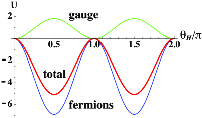
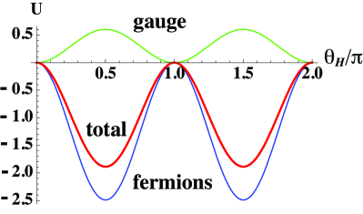
Figure 1: The effective potential $V_{\rm eff}(\theta_{H})$ in the model. The plot is for $U(\theta_{H}/\pi)=(4\pi)^{2}(kz_{L}^{-1})^{-4}\,V_{\rm eff}$ at $z_{L}=10^{5}$ (left) and $z_{L}=10^{15}$ (right). Green, blue, and red curves represent $V_{\rm eff}^{\rm gauge}$, $V_{\rm eff}^{\rm fermion}$, and $V_{\rm eff}$, respectively. The global minima are located at $\theta_{H}=\hbox{${1\over 2}$}\pi$ and $\frac{3}{2}\pi$, where the EW symmetry dynamically breaks down to $U(1)_{{\rm EM}}$.

We observe that

$$V_{\rm eff}(\theta_{H}+\pi)=V_{\rm eff}(\theta_{H})=V_{\rm eff}(-\theta_{H})~{}.$$ (4.12)

It is important in the first equality that all bulk fermions are introduced in the vector representation of $SO(5)$. If there were a bulk fermion, say, in the spinor representation of $SO(5)$, the $\theta_{H}$-dependence in $I$ in (4.11) would contain $\sin^{2}\hbox{${1\over 2}$}\theta_{H}$ instead of $\sin^{2}\theta_{H}$. If all bulk fermions were in the spinor representation, the minimum of $V_{\rm eff}$ would be located either at $\theta=0$ or $\pi$ so that the EW symmetry would be unbroken.

We also remark that the scale of the depth of the effective potential is given by $m_{\rm KK}/(2\pi^{3/2})$. As the universe expands and cools down, the electroweak symmetry breaking is expected to take place at a temperature of the electroweak scale. To determine the precise value one needs to evaluate the effective potential at finite temperature.

The mass of the 4D neutral Higgs boson is determined from the curvature of the effective potential at the minimum. Making use of (2.14), one finds

$$m_{H}^{2}=\frac{1}{f_{H}^{2}}\frac{d^{2}V_{\rm eff}}{d\theta_{H}^{2}}\bigg{|}_{\theta_{H}=\hbox{${1\over 2}$}\pi}~{}.$$ (4.13)

It follows from (4.11) that

$$\hskip-28.45274ptm_{H}^{2}\simeq\frac{g_{w}^{2}kLm_{\rm KK}^{2}}{64\pi^{4}}\bigg{\{}-4G[\hbox{${1\over 2}$}\bar{Q}_{0}(q,\hbox{${1\over 2}$})]-2G\Big{[}\frac{1}{2\cos^{2}\theta_{W}}\bar{Q}_{0}(q,\hbox{${1\over 2}$})\Big{]}-3G[\bar{Q}_{0}(q,\hbox{${1\over 2}$})]$$ (4.14)

$$\hskip 42.67912pt+12\sum_{\rm quarks}\bigg{(}G\Big{[}\frac{1}{2(1+r_{q})}\bar{Q}_{0}(q,c_{q})\Big{]}+G\Big{[}\frac{r_{q}}{2(1+r_{q})}\bar{Q}_{0}(q,c_{q})\Big{]}\bigg{)}$$ (4.15)

$$\hskip 42.67912pt+4\sum_{\rm leptons}\bigg{(}G\Big{[}\frac{1}{2(1+r_{\ell})}\bar{Q}_{0}(q,c_{\ell})\Big{]}+G\Big{[}\frac{r_{\ell}}{2(1+r_{\ell})}\bar{Q}_{0}(q,c_{\ell})\Big{]}\bigg{)}\bigg{\}}~{},$$ (4.16)

$$\hskip-28.45274ptG[f(q)]=\int_{0}^{\infty}dq\,q^{3}\frac{2f(q)}{1+f(q)}~{}~{},~{}~{}\bar{Q}_{0}(q,c)\equiv Q_{0}(q;c,\hbox{${1\over 2}$}\pi)~{}~{}.$$ (4.17)

Among fermion multiplets, only the top quark multiplet gives an appreciable contribution. The result is summarized in Table 2.

Higgs bosons become stable in the model. They can become the dark matter in the universe. It was shown in ref. [29] that the mass density of the dark matter determined by the WMAP data is reproduced with $m_{H}\sim 70\,$GeV. This value of $m_{H}$ is obtained with $z_{L}\sim 10^{5}$ in the current model.

$z_{L}=e^{kL}$	$\sin^{2}\theta_{W}$	$k$(GeV)	$m_{\rm KK}$(GeV)	$c_{\rm top}$	$m_{H}$(GeV)	$m_{W}^{\rm tree}$(GeV)
$10^{15}$	0.2312	$4.666\times 10^{17}$	1,466	0.432	135	79.82
$10^{10}$	0.23	$3.799\times 10^{12}$	1,194	0.396	108	79.82
$10^{5}$	0.2285	$2.662\times 10^{7}$	836	0.268	72	79.70

Table 2: The Higgs boson mass $m_{H}$. Relevant input parameters are $m_{Z}=91.1876\,$GeV, $\alpha_{w}=1/128$ and $m_{t}=171.17\,$GeV. The AdS curvature $k$ and $W$ mass at the tree level are also listed.

It is curious to examine whether or not the EW symmetry is broken in the flat spacetime limit. As shown in ref. [27] the top quark mass $m_{t}\sim 170\,$GeV cannot be realized for $z_{L}<900$. It is possible to consider the flat spacetime limit ($k\rightarrow 0,~{}z_{L}\rightarrow 1$) by taking the bulk mass $c=0$ for the top quark multiplet. It is found that around $z_{L}^{c}\sim 1.67$ the phase transition takes place. The transition is weakly first-order. Below $z_{L}$ the global minima of $V_{\rm eff}$ are located at $\theta_{H}=0,\pi$ where the EW symmetry remains unbroken. See fig. 2.

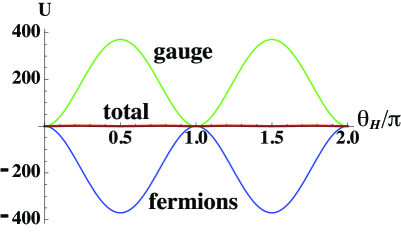
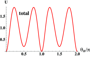
Figure 2: The critical behavior near $z_{L}=1.67$, below which $V_{\rm eff}$ is minimized at $\theta_{H}=0,\pi$.

5 Enhanced gauge invariance

In this section we show that the theory is invariant under the shift $\theta_{H}\rightarrow\theta_{H}+\pi$ to all order in perturbation theory. In other words the physics is periodic in $\theta_{H}$ with a period $\pi$. This property follows from the enhanced gauge invariance in the model in which (i) the bulk fermions are all in the vector representation of $SO(5)$, and (ii) the brane fermions and brane scalar are introduced only on one of the two branes, say, on the Planck brane.

To see it we consider an $SO(5)$ gauge transformation $A_{M}^{\prime}=\Omega A_{M}\Omega^{-1}+(i/g_{A})\Omega\partial_{M}\Omega^{-1}$ where

$$\Omega(y;\alpha)=\exp\Big{\{}i\alpha q(y)\,T^{\hat{4}}\Big{\}}~{}~{},~{}~{}q(y)=g_{A}f_{H}\int_{0}^{y}dy^{\prime}\,u_{H}(y^{\prime})~{}~{}.$$ (5.1)

$u_{H}(y)$ in $0\leq y\leq L$ is given by (2.14), and is extended in other regions by $u_{H}(-y)=u_{H}(y)=u_{H}(y+2L)$. It follows that

$$q(y)+q(-y)=0~{}~{},~{}~{}q(L+y)+q(L-y)=2\sqrt{2}~{}.$$ (5.2)

In the fundamental region $0\leq y\leq L$

$$\Omega(y;\alpha)=\exp\bigg{\{}i\sqrt{2}\,\alpha\,\frac{e^{2ky}-1}{z_{L}^{2}-1}\,T^{\hat{4}}\bigg{\}}~{}.$$ (5.3)

This gauge transformation shifts the Wilson line phase $\theta_{H}$ to $\theta_{H}^{\prime}=\theta_{H}+\alpha$. The fields in the new gauge satisfy the boundary condition (2.11) with $P_{j}$ replaced by $P_{j}(\alpha)=\Omega(y_{j}-y;\alpha)P_{j}\Omega(y_{j}+y;\alpha)^{-1}$. Note that $P_{j}(\alpha)$ is independent of $y$.

In the vectorial representation $P_{j}={\rm diag~{}}(-1,-1,-1,-1,1)$ and $(T^{\hat{4}})_{ab}=(i/\sqrt{2})(\delta_{a5}\delta_{b4}-\delta_{a4}\delta_{b5})$ so that $P_{0}(\pi)=P_{0}$ and $P_{1}(\pi)=P_{1}$. In the spinorial representation $P_{j}=I_{2}\otimes\tau_{3}$ and $T^{\hat{4}}=(1/2\sqrt{2})I_{2}\otimes\tau_{1}$ so that $P_{0}(\pi)=P_{0}$ and $P_{1}(\pi)=-P_{1}$. As $\Omega(0;\alpha)=1$, the brane fermions and scalar are not affected by this gauge transformation. It follows that the model under consideration is invariant under the large gauge transformation $\Omega(y;\pi)$, that is to say, the theory is periodic in $\theta_{H}$ with a period $\pi$. It implies, for instance, that $V_{\rm eff}(\theta_{H}+\pi)=V_{\rm eff}(\theta_{H})$ to all order in perturbation theory. The mirror reflection symmetry under $y\rightarrow-y$ leads to $V_{\rm eff}(-\theta_{H})=V_{\rm eff}(\theta_{H})$. Combining these two, one finds that $V_{\rm eff}(\theta_{H})$ is symmetric around $\theta_{H}=\pm\hbox{${1\over 2}$}\pi$ to all order in perturbation theory. In the previous section we have observed that $V_{\rm eff}(\theta_{H})$ is minimized at $\theta_{H}=\pm\hbox{${1\over 2}$}\pi$ at the one-loop level. The location of the minimum will not be shifted in one direction by radiative corrections. $\theta_{H}=\pm\hbox{${1\over 2}$}\pi$ remains as an extremum of $V_{\rm eff}$.

We stress that the above property would be lost if there were, for instance, a bulk fermion in the spinor representation of $SO(5)$. Furthermore $\Omega(L;\pi)=\exp\{i\sqrt{2}\pi T^{\hat{4}}\}\not=1$ in either vectorial or spinorial representation. If brane fields were introduced on the TeV brane at $y=L$ as well as on the Planck brane at $y=0$, then the enhanced periodicity would be lost in general. In passing $\Omega(L;2\pi)=1$ or $-1$ in the vectorial or spinorial representation, respectively.

6 $H$ parity

We expand all fields around the vacuum $\theta_{H}=\hbox{${1\over 2}$}\pi$. It has been shown in ref. [29] that the $H$ parity ($P_{H}$) conservation results among the low energy fields as a result of the enhanced gauge invariance and the mirror reflection symmetry in the fifth dimension. The neutral physical Higgs boson is $P_{H}$ odd, whereas all other particles in the standard model are $P_{H}$ even. It follows that the lightest $P_{H}$ odd particle, the Higgs boson, is absolutely stable.

A natural question arises as to whether all fields including KK modes can be classified with respect to $P_{H}$. We show that one can assign definite $H$ parity to all fields at $\theta_{H}=\hbox{${1\over 2}$}\pi$ and that both the bulk action (2.5) and the brane action (2.27) are invariant under $P_{H}$. As we shall see below, $P_{H}$ interchanges $SU(2)_{L}$ and $SU(2)_{R}$ and flips the sign of $T^{\hat{4}}$. The $P_{H}$ symmetry is similar to the $P_{LR}$ symmetry discussed by Agashe, Contino, Da Rold and Pomarol [17], which protects the $Zb\bar{b}$ coupling from radiative corrections.

The KK expansions of the gauge fields have been worked out in ref. [19]. In the expansion on orbifolds with topology of $M^{4}\times(S^{1}/Z_{2})$, there appear two types of the sums. The number of degrees of freedom on $S^{1}/Z_{2}$ is halved compared with that on $S^{1}$. For those fields which acquire masses by the Hosotani mechanism ($\theta_{H}\not=0$) two degrees of freedom combine to form one set of towers as depicted in Fig. 3 with the sum $\sum^{d}$. On flat $S^{1}$ it corresponds to combining cosine and sine series for $\theta_{H}=0$. It contains a zero mode at $\theta_{H}=0$. In the Randall-Sundrum warped space there appears a gap in the spectrum between the two branches (corresponding the cosine and sine series in flat space) even at $\theta_{H}=0$. The other type of a spectrum is independent of $\theta_{H}$, as depicted in Fig. 3 with the sum $\sum^{s}$. There may or may not be a zero mode. From the viewpoint of the number of degrees of freedom, $\sum^{d}$ counts two KK towers, whereas $\sum^{s}$ counts one KK tower.

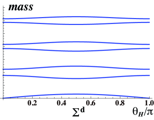
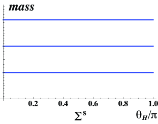
Figure 3: Two types of spectra where the horizontal axis is $\theta_{H}/\pi$.

(i) Gauge fields

Following refs. [19] and [32], we expand the gauge fields in the twisted gauge, in which $\raise 0.68889pt\hbox{$\langle$}\lower 0.68889pt\hbox{}\tilde{A}_{y}\raise 0.68889pt\hbox{$\rangle$}\lower 0.68889pt\hbox{}=0$, as

$$\tilde{A}_{\mu}(x,z) \!\!\!=\!\!\! \sum_{n=0}^{\infty}{}^{d}\,W_{\mu}^{(n)}\left\{N_{W}(\lambda_{n}){T^{-_{L}}+T^{-_{R}}\over 2}+\cos\theta_{H}N_{W}(\lambda_{n}){T^{-_{L}}-T^{-_{R}}\over 2}\right.$$ (6.7)

$$\hskip 85.35826pt\left.-{\sin\theta_{H}\over\sqrt{2}}D_{W}(\lambda_{n})T^{\hat{-}}\right\}+\textrm{h.c.}$$

$$\hskip-28.45274pt+\sum_{n=1}^{\infty}{}^{s}\,W_{\mu}^{{}^{\prime}(n)}\left\{-\cos\theta_{H}N_{W^{\prime}}(\lambda_{n}){T^{-_{L}}+T^{-_{R}}\over 2}+N_{W^{\prime}}(\lambda_{n}){T^{-_{L}}-T^{-_{R}}\over 2}\right\}+\textrm{h.c.}$$

$$\hskip-28.45274pt+\sum_{n=0}^{\infty}{}^{s}\,A_{\mu}^{\gamma(n)}h_{\gamma}(\lambda_{n})(T^{3_{L}}+T^{3_{R}})+\sum_{n=1}^{\infty}{}^{s}A_{\mu}^{\hat{4}(n)}h_{A}(\lambda_{n})T^{\hat{4}}$$

$$\hskip-28.45274pt+\sum_{n=0}^{\infty}{}^{d}\,Z_{\mu}^{(n)}\bigg{\{}\frac{c_{\phi}^{2}}{\sqrt{1+s_{\phi}^{2}}}N_{Z}(\lambda_{n}){T^{3_{L}}+T^{3_{R}}\over 2}+\cos\theta_{H}\sqrt{1+s_{\phi}^{2}}N_{Z}(\lambda_{n}){T^{3_{L}}-T^{3_{R}}\over 2}$$

$$\hskip 85.35826pt-{\sin\theta_{H}\over\sqrt{2}}\sqrt{1+s_{\phi}^{2}}D_{Z}(\lambda_{n})T^{\hat{3}}\bigg{\}}$$

$$\hskip-28.45274pt+\sum_{n=1}^{\infty}{}^{s}Z_{\mu}^{{}^{\prime}(n)}\left\{-\cos\theta_{H}N_{Z^{\prime}}(\lambda_{n}){T^{3_{L}}+T^{3_{R}}\over 2}+N_{Z^{\prime}}(\lambda_{n}){T^{3_{L}}-T^{3_{R}}\over 2}\right\}~{},$$

$$\tilde{B}_{\mu}(x,z) \!\!\!=\!\!\! \sum_{n=0}^{\infty}{}^{s}A_{\mu}^{\gamma(n)}{c_{\phi}\over s_{\phi}}h_{\gamma n}-\sum_{n=0}^{\infty}{}^{d}Z_{\mu}^{(n)}\frac{s_{\phi}c_{\phi}}{\sqrt{1+s_{\phi}^{2}}}N_{Z}(\lambda_{n})$$ (6.9)

$$\hskip 85.35826pt+\sum_{n=1}^{\infty}{}^{s}Z_{\mu}^{{}^{\prime}(n)}\cos\theta_{H}{s_{\phi}\over c_{\phi}}N_{Z^{\prime}}(\lambda_{n})~{}.$$

Here $T^{\pm}=(T^{1}\pm iT^{2})/\sqrt{2}$, $c_{\phi}=g_{A}/\sqrt{g_{A}^{2}+g_{B}^{2}}$ and $s_{\phi}=g_{B}/\sqrt{g_{A}^{2}+g_{B}^{2}}$. The mixing angle between $SO(5)$ and $U(1)_{X}$ is related to the Weinberg angle as $\sin^{2}\theta_{W}\equiv s_{\phi}^{2}/(1+s_{\phi}^{2})$. The $n=0$ mode stands for the zeroth mode which is massless at $\theta_{H}=0$. $A_{\mu}^{\gamma(0)}$ remains massless at all $\theta_{H}$. The $W$ and $Z$ bosons and the photon $\gamma$ correspond to $W_{\mu}^{(0)}$, $Z_{\mu}^{(0)}$ and $A_{\mu}^{\gamma(0)}$, respectively. Unless confusion arises, we will omit the superscript $(0)$ for representing the lowest mode. The mode functions $N_{W}(\lambda)=N_{W}(z,\lambda)$, $D_{W}(\lambda)=D_{W}(z,\lambda)$ etc. are expressed in terms of Bessel functions

$$\hskip-28.45274ptC(z;\lambda)={\pi\over 2}\lambda zz_{L}F_{1,0}(\lambda z,\lambda z_{L})~{},\quad C^{\prime}(z;\lambda)={\pi\over 2}\lambda^{2}zz_{L}F_{0,0}(\lambda z,\lambda z_{L})~{},$$ (6.10)

$$\hskip-28.45274ptS(z;\lambda)=-{\pi\over 2}\lambda zF_{1,1}(\lambda z,\lambda z_{L})~{},\quad S^{\prime}(z;\lambda)=-{\pi\over 2}\lambda^{2}zF_{0,1}(\lambda z,\lambda z_{L})~{},$$ (6.11)

$$\hskip-28.45274ptF_{\alpha,\beta}(u,v)=J_{\alpha}(u)Y_{\beta}(v)-Y_{\alpha}(u)J_{\beta}(v)~{}.$$ (6.12)

$N,h_{\gamma}\propto C(z;\lambda)$ and $D,h_{A}\propto S(z;\lambda)$ where proportionality constants are given in ref. [32]. For the photon ($\lambda_{0}=0$), $C(z;0)$ is constant.

The mass spectrum $m_{n}=k\lambda_{n}$ of each KK tower is determined by the corresponding eigenvalue equations:

$$W_{\mu}^{(n)} : 2S(1;\lambda_{n})C^{\prime}(1;\lambda_{n})+\lambda_{n}\sin^{2}\theta_{H}=0~{},$$ (6.13)

$$W_{\mu}^{{}^{\prime}(n)} : C(1;\lambda_{n})=0~{},$$ (6.14)

$$Z_{\mu}^{(n)} : 2S(1;\lambda_{n})C^{\prime}(1;\lambda_{n})+\lambda_{n}(1+s_{\phi}^{2})\sin^{2}\theta_{H}=0~{},$$ (6.15)

$$Z_{\mu}^{{}^{\prime}(n)} : C(1;\lambda_{n})=0~{},$$ (6.16)

$$A_{\mu}^{\gamma(n)} : C^{\prime}(1;\lambda_{n})=0~{},$$ (6.17)

$$A_{\mu}^{\hat{4}(n)} : S(1;\lambda_{n})=0~{}.$$ (6.18)

At $\theta_{H}=\hbox{${1\over 2}$}\pi$, the Weinberg angle $\theta_{W}$ is determined by global fit of various quantities. With $m_{Z}$ and $z_{L}$ as an input, the AdS curvature $k$ and the $W$ boson mass at the tree level are determined as in Table 2. Counting the number of mass eigenvalue equations in (6.18), one finds that the 11 degrees of freedom for the original $SO(5)\times U(1)_{X}$ gauge fields $\tilde{A}_{\mu}$ and $\tilde{B}_{\mu}$ are decomposed into charged components, 4 $W_{\mu}^{(n)}$ and 2 $W_{\mu}^{\prime(n)}$, and neutral components, 2 $Z_{\mu}^{(n)}$, 1 $Z_{\mu}^{\prime(n)}$, 1 $A_{\mu}^{\gamma(n)}$ and 1 $A_{\mu}^{\hat{4}(n)}$.

Similarly the fifth-dimensional components $A_{z}$ and $B_{z}$ are expanded as

$$\hskip-28.45274pt\tilde{A}_{z}(x,z)=\sum_{n=1}^{\infty}{}^{s}\sum_{a=1}^{3}S^{a(n)}h_{S}^{LR}(\lambda_{n})\frac{T^{a_{L}}+T^{a_{R}}}{\sqrt{2}}+\sum_{n=0}^{\infty}{}^{s}H^{(n)}h_{H}^{\wedge}(\lambda_{n})T^{\hat{4}}$$ (6.19)

$$\hskip-14.22636pt+\sum_{n=1}^{\infty}{}^{d}\sum_{a=1}^{3}D^{a(n)}\bigg{\{}v_{n}(\theta_{H},\lambda_{n})h_{D}^{LR}(\lambda_{n})\frac{T^{a_{L}}-T^{a_{R}}}{\sqrt{2}}+w_{n}(\theta_{H},\lambda_{n})h_{D}^{\wedge}(\lambda_{n})T^{\hat{a}}\bigg{\}}~{},$$ (6.20)

$$\hskip-28.45274pt\tilde{B}_{z}(x,z)=\sum_{n=1}^{\infty}{}^{s}B^{(n)}h_{B}(\lambda_{n})~{}.$$ (6.21)

Here $h_{S}^{LR},h_{D}^{LR},h_{B}\propto C^{\prime}(z;\lambda)$ and $h_{H}^{\wedge},h_{D}^{\wedge}\propto S^{\prime}(z;\lambda)$. $H(x)=H^{(0)}(x)$ is the 4D neutral Higgs boson. The wave functions of $D^{a(n)}$ are rather involved. The mass spectrum of each KK tower is given by

$$S^{a(n)} : C^{\prime}(1;\lambda_{n})=0~{},$$ (6.22)

$$B^{(n)} : C^{\prime}(1;\lambda_{n})=0~{},$$ (6.23)

$$D^{a(n)} : S(1;\lambda_{n})C^{\prime}(1;\lambda_{n})+\lambda_{n}\sin^{2}\theta_{H}$$ (6.25)

$$=C(1;\lambda_{n})S^{\prime}(1;\lambda_{n})-\lambda_{n}\cos^{2}\theta_{H}=0~{},$$

$$H^{(n)} : S(1;\lambda_{n})=0~{},$$ (6.26)

The 11 degrees of freedom for the original $SO(5)\times U(1)$ gauge fields $\tilde{A}_{z}$ and $\tilde{B}_{z}$ are decomposed into 3 $S^{(n)}$, 6 $D^{(n)}$, 1 $H^{(n)}$ and 1 $B^{(n)}$.

At $\theta_{H}=\hbox{${1\over 2}$}\pi$ the KK expansion of $\tilde{A}_{z}$ takes a simpler form. The modes $\{D^{a(n)}\}$ split into two classes;

$$\hskip-28.45274pt\tilde{A}_{z}(x,z)=\sum_{n=1}^{\infty}{}^{s}\sum_{a=1}^{3}S^{a(n)}h_{S}^{LR}(\lambda_{n})\frac{T^{a_{L}}+T^{a_{R}}}{\sqrt{2}}+\sum_{n=0}^{\infty}{}^{s}H^{(n)}h_{H}^{\wedge}(\lambda_{n})T^{\hat{4}}$$ (6.27)

$$\hskip 0.0pt+\sum_{n=1}^{\infty}{}^{s}\sum_{a=1}^{3}D_{-}^{a(n)}h_{D}^{LR}(\lambda_{n})\frac{T^{a_{L}}-T^{a_{R}}}{\sqrt{2}}+\sum_{n=1}^{\infty}{}^{s}\sum_{a=1}^{3}\hat{D}^{a(n)}h_{D}^{\wedge}(\lambda_{n})T^{\hat{a}}~{},$$ (6.28)

$$\hskip 28.45274ptD_{-}^{a(n)}~{}:~{}C(1;\lambda_{n})=0~{},$$ (6.29)

$$\hskip 28.45274pt\hat{D}^{a(n)}~{}:~{}S^{\prime}(1;\lambda_{n})=0~{}.$$ (6.30)

At this stage we recall the algebra of the generators $\{T^{\alpha}\}$ of $SO(5)$;

$$\hskip-28.45274pt[T^{a_{L}},T^{b_{L}}]=i\epsilon^{abc}T^{c_{L}}~{}~{},~{}~{}[T^{a_{R}},T^{b_{R}}]=i\epsilon^{abc}T^{c_{R}}~{}~{},~{}~{}[T^{a_{L}},T^{b_{R}}]=0~{}~{},$$ (6.31)

$$\hskip-28.45274pt[T^{\hat{a}},T^{\hat{b}}]=\frac{i}{2}\epsilon^{abc}(T^{c_{L}}+T^{c_{R}})~{}~{},~{}~{}$$ (6.32)

$$\hskip-28.45274pt[T^{\hat{a}},T^{b_{L}}]=-\frac{i}{2}\delta^{ab}T^{\hat{4}}+\frac{i}{2}\epsilon^{abc}T^{\hat{c}}~{}~{},~{}~{}[T^{\hat{a}},T^{b_{R}}]=+\frac{i}{2}\delta^{ab}T^{\hat{4}}+\frac{i}{2}\epsilon^{abc}T^{\hat{c}}~{}~{},$$ (6.33)

$$\hskip-28.45274pt[T^{a_{L}},T^{\hat{4}}]=-\frac{i}{2}T^{\hat{a}}~{}~{},~{}~{}[T^{a_{R}},T^{\hat{4}}]=+\frac{i}{2}T^{\hat{a}}~{}~{},~{}~{}[T^{\hat{a}},T^{\hat{4}}]=\frac{i}{2}(T^{a_{L}}-T^{a_{R}})~{}~{},$$ (6.34)

$$\hskip 56.9055pt(a,b,c=1\sim 3)~{}.$$ (6.35)

The explicit matrix representations of $\{T^{\alpha}\}$ are given in ref. [13]. The algebra remains invariant under the substitution of $\{T^{\alpha}\}=\{T^{a_{L}},T^{a_{R}},T^{\hat{a}},T^{\hat{4}}\}$ by $\{T^{\prime\alpha}\}=\{T^{a_{R}},T^{a_{L}},T^{\hat{a}},-T^{\hat{4}}\}$. The two sets are related to each other by an $O(5)$ transformation $T^{\prime\alpha}=\Omega_{H}T^{\alpha}\Omega_{H}^{-1}$ where $\Omega_{H}={\rm diag}\,(1,1,1,-1,1)$ in the vectorial representation. $\Omega_{H}$ interchanges $SU(2)_{L}$ and $SU(2)_{R}$ and flips the direction of $T^{\hat{4}}$.

At $\theta_{H}=\hbox{${1\over 2}$}\pi$ ($\cos\theta_{H}=0$) additional symmetry arises in the expansions. Look at, for instance, $W_{\mu}^{(n)}$ and $W_{\mu}^{\prime(n)}$ terms in (6.9). At $\theta_{H}=\hbox{${1\over 2}$}\pi$ the $W_{\mu}^{(n)}$ terms are invariant under $\Omega_{H}$, whereas the $W_{\mu}^{\prime(n)}$ term flips the sign. Indeed, $\Omega_{H}\tilde{A}_{M}(x,z)\Omega_{H}^{-1}$ is the same as $\tilde{A}_{M}(x,z)$ where the signs of the fields

$$W^{\prime(n)}_{\mu},Z^{\prime(n)}_{\mu},A_{\mu}^{\hat{4}(n)},H^{(n)},D_{-}^{a(n)}\quad(P_{H}~{}\hbox{odd})$$ (6.36)

are flipped. This defines $H$ parity ($P_{H}$) for all 4D fields. 4D fields contained in $\tilde{A}_{M}$ other than those in (6.36) are $P_{H}$ even.

The action of the pure gauge fields in the bulk, ${\rm Tr\,}F_{MN}F^{MN}$, is invariant under the $\Omega_{H}$ transformation so that it is invariant under $H$ parity. We show below that the invariance holds for the entire action including the bulk fermions, brane fermions, and brane scalar.

(ii) Fermions

$H$ parity of fermions is determined in the following manner. Consider the fermion multiplets containing quarks, namely, $\Psi_{1}$ and $\Psi_{2}$ in (2.18) and ${\hat{\chi}}^{q}_{1R}$, ${\hat{\chi}}^{q}_{2R}$, ${\hat{\chi}}^{q}_{3R}$, in (2.21). They are classified in terms of electric charge $Q_{E}=\frac{5}{3}$, $\frac{2}{3}$, $-\frac{1}{3}$, $-\frac{4}{3}$. Recall that components of $\check{\Psi}$ in (2.18) are related to the components $\Psi^{k}$ ($k=1\sim 5$) in the vectorial representation by

$$\check{\Psi}=\begin{pmatrix}\check{\Psi}_{11}&\check{\Psi}_{12}\cr\check{\Psi}_{21}&\check{\Psi}_{22}\end{pmatrix}=-\frac{1}{\sqrt{2}}\begin{pmatrix}\Psi^{2}+i\Psi^{1}&-\Psi^{4}-i\Psi^{3}\\ \Psi^{4}-i\Psi^{3}&\Psi^{2}-i\Psi^{1}\\ \end{pmatrix}~{}.$$ (6.37)

Only $\Psi^{4}$ and $\Psi^{5}$ couple with $\theta_{H}$. By $\Omega_{H}$ the bulk fermions are transformed, in the twisted gauge, to $\tilde{\Psi}(x,z)\rightarrow\Omega_{H}\tilde{\Psi}(x,z)$. In the vectorial representation $(\tilde{\Psi}^{1},\tilde{\Psi}^{2},\tilde{\Psi}^{3},\tilde{\Psi}^{4},\tilde{\Psi}^{5})\rightarrow(\tilde{\Psi}^{1},\tilde{\Psi}^{2},\tilde{\Psi}^{3},-\tilde{\Psi}^{4},\tilde{\Psi}^{5})$.

The $Q_{E}=\frac{5}{3}$ sector consists of $T$ in $\Psi_{1}$ and $\hat{T}_{R}$ in $\hat{\chi}^{q}_{1R}$. These fields do not couple to $\theta_{H}$ so that the spectrum and mode functions are independent of $\theta_{H}$. The 4D fields in this sector are all $P_{H}$ even.

The $Q_{E}=\frac{2}{3}$ sector consists of $B$, $t$, $t^{\prime}$ in $\Psi_{1}$, $U$ in $\Psi_{2}$, $\hat{B}_{R}$ in $\hat{\chi}^{q}_{1R}$ and $\hat{U}_{R}$ in $\hat{\chi}^{q}_{2R}$. These fields are intertwined by $\theta_{H}\not=0$. The spectrum and wave functions of the low-lying modes have been given in refs. [27, 28, 32]. The arguments can be generalized to KK modes as well.

The boundary conditions at the TeV brane demand that the left- and right-handed fields are expanded in the twisted gauge as

$$\begin{pmatrix}\tilde{U}_{L}\\ (\tilde{B}_{L}\pm\tilde{t}_{L})/\sqrt{2}\\ \tilde{t}_{L}^{\prime}\end{pmatrix}(x,z) \!\!\!=\!\!\! \sqrt{k}\sum_{n}\begin{pmatrix}a_{U}^{(n)}C_{L}(z;\lambda_{n},c_{2})\\ a_{B\pm t}^{(n)}C_{L}(z;\lambda_{n},c_{1})\\ a_{t^{\prime}}^{(n)}S_{L}(z;\lambda_{n},c_{1})\end{pmatrix}\psi^{(n)}_{\frac{2}{3},L}(x)~{},$$ (6.38)

$$\begin{pmatrix}\tilde{U}_{R}\\ (\tilde{B}_{R}\pm\tilde{t}_{R})/\sqrt{2}\\ \tilde{t}_{R}^{\prime}\end{pmatrix}(x,z) \!\!\!=\!\!\! \sqrt{k}\sum_{n}\begin{pmatrix}a_{U}^{(n)}S_{R}(z;\lambda_{n},c_{2})\\ a_{B\pm t}^{(n)}S_{R}(z;\lambda_{n},c_{1})\\ a_{t^{\prime}}^{(n)}C_{R}(z;\lambda_{n},c_{1})\end{pmatrix}\psi^{(n)}_{\frac{2}{3},R}(x)~{}.$$ (6.39)

Here $c_{a}$ is the bulk kink mass for $\Psi_{a}$, and

$$\hskip-28.45274pt\begin{pmatrix}C_{L}\cr S_{L}\end{pmatrix}(z;\lambda,c)=\pm\frac{\pi}{2}\lambda\sqrt{zz_{L}}F_{c+{1\over 2},c\mp{1\over 2}}(\lambda z,\lambda z_{L})~{},$$ (6.40)

$$\hskip-28.45274pt\begin{pmatrix}C_{R}\cr S_{R}\end{pmatrix}(z;\lambda,c)=\mp\frac{\pi}{2}\lambda\sqrt{zz_{L}}F_{c-{1\over 2},c\pm{1\over 2}}(\lambda z,\lambda z_{L})~{}.$$ (6.41)

The brane fields $\hat{B}_{R}$ and $\hat{U}_{R}$ can be expressed in terms of the bulk fields.

The boundary conditions at the Planck brane lead to a matrix equation

$$K~{}\begin{pmatrix}a_{U}^{(n)}\cr{\displaystyle 1\over\displaystyle 2}~{}a_{B+t}^{(n)}\cr{\displaystyle 1\over\displaystyle\sqrt{2}}~{}a_{t^{\prime}}^{(n)}\cr{\displaystyle 1\over\displaystyle 2}~{}a_{B-t}^{(n)}\end{pmatrix}=0~{},$$ (6.42)

where

$$\hskip-28.45274ptK=$$ (6.43)

$$\hskip-28.45274pt\begin{pmatrix}0&0&-2c_{H}S_{L}^{(1)}&2s_{H}C_{L}^{(1)}\cr\lambda_{n}S_{R}^{(2)}-{\displaystyle\mu_{2}^{2}\over\displaystyle 2k}C_{L}^{(2)}&-{\displaystyle\mu_{2}\tilde{\mu}\over\displaystyle 2k}C_{L}^{(1)}&s_{H}{\displaystyle\mu_{2}\tilde{\mu}\over\displaystyle 2k}S_{L}^{(1)}&{\displaystyle\mu_{2}\tilde{\mu}\over\displaystyle 2k}c_{H}C_{L}^{(1)}\cr 0&\lambda_{n}S_{R}^{(1)}-{\displaystyle\mu_{1}^{2}\over\displaystyle 2k}C_{L}^{(1)}&s_{H}\big{(}\lambda_{n}C_{R}^{(1)}-{\displaystyle\mu_{1}^{2}\over\displaystyle 2k}S_{L}^{(1)}\big{)}&c_{H}\big{(}\lambda_{n}S_{R}^{(1)}-{\displaystyle\mu_{1}^{2}\over\displaystyle 2k}C_{L}^{(1)}\big{)}\cr-{\displaystyle\mu_{2}\tilde{\mu}\over\displaystyle 2k}C_{L}^{(2)}&\lambda_{n}S_{R}^{(1)}-{\displaystyle\tilde{\mu}^{2}\over\displaystyle 2k}C_{L}^{(1)}&-s_{H}\big{(}\lambda_{n}C_{R}^{(1)}-{\displaystyle\tilde{\mu}^{2}\over\displaystyle 2k}S_{L}^{(1)}\big{)}&-c_{H}\big{(}\lambda_{n}S_{R}^{(1)}-{\displaystyle\tilde{\mu}^{2}\over\displaystyle 2k}C_{L}^{(1)}\big{)}\end{pmatrix}.$$ (6.44)

(6.45)

Here $s_{H}=\sin\theta_{H},c_{H}=\cos\theta_{H}$, $C_{L,R}^{(j)}=C_{L,R}(1;\lambda_{n},c_{j})$ and $S_{L,R}^{(j)}=S_{L,R}(1;\lambda_{n},c_{j})$.

Nontrivial solutions exist with $\det K=0$, which determines the spectrum. At $\theta_{H}=\hbox{${1\over 2}$}\pi$, special structure appears. Eq. (6.42) leads to

$$C_{L}(1;\lambda_{n},c_{1})a_{B-t}^{(n)}=0~{}.$$ (6.46)

Solutions with $C_{L}(1;\lambda_{n},c_{1})=0$ have $a_{B-t}^{(n)}\not=0$ and $a_{U}^{(n)}=a_{B+t}^{(n)}=a_{t^{\prime}}^{(n)}=0$. The corresponding 4D fermion tower is denoted as $\psi_{B-t}^{(n)}(x)$. As the component $\tilde{B}-\tilde{t}$ is $\tilde{\Psi}_{1}^{4}$, it flips the sign under the $\Omega_{H}$ transformation. The KK tower $\psi_{B-t}^{(n)}(x)$ is $P_{H}$ odd. We note that the mode function of the left-handed $\psi_{B-t,L}^{(n)}(x)$ vanishes at $z=1$, while that of the right-handed $\psi_{B-t,R}^{(n)}(x)$ is non-vanishing as seen from (6.39). For $C_{L}(1;\lambda_{n},c_{1})\not=0$, $a_{B-t}^{(n)}=0$. The spectrum and mode functions are determined by the 3-by-3 matrix equation reduced from (6.42). They give three KK towers of 4D fermions, including the tower of the top quark. As $\tilde{B}+\tilde{t}\sim\tilde{\Psi}_{1}^{3}$, $\tilde{t}^{\prime}\sim\tilde{\Psi}_{1}^{5}$ and $\tilde{U}\sim\tilde{\Psi}_{2}^{2}+i\tilde{\Psi}_{2}^{1}$, these three KK towers are all $P_{H}$ even. The brane fermions $\hat{B}_{R}$ and $\hat{U}_{R}$ are related to the bulk fermions by

$$\hskip-28.45274pt{\displaystyle\mu_{1}\over\displaystyle 2}\hat{B}_{R}=B_{R}\big{|}_{z=1}={\displaystyle 1\over\displaystyle 2}(\tilde{B}_{R}+\tilde{t}_{R})+\frac{1}{\sqrt{2}}\,\tilde{t}_{R}^{\prime}~{}\bigg{|}_{z=1}~{},$$ (6.47)

$$\hskip-28.45274pt{\displaystyle\mu_{2}\over\displaystyle 2}\hat{U}_{R}=U_{R}\big{|}_{z=1}=\tilde{U}_{R}\big{|}_{z=1}~{}.$$ (6.48)

They contain only $P_{H}$ even fields.

Parallel arguments apply to the $Q_{E}=-\frac{1}{3}$ sector, which consists of $b$ in $\Psi_{1}$, $D,X,b^{\prime}$ in $\Psi_{2}$, $\hat{D}_{R}$ in $\hat{\chi}^{q}_{2R}$ and $\hat{X}_{R}$ in $\hat{\chi}^{q}_{3R}$. The bulk fields are expanded as

$$\begin{pmatrix}\tilde{b}_{L}\\ (\tilde{D}_{L}\pm\tilde{X}_{L})/\sqrt{2}\\ \tilde{b}_{L}^{\prime}\end{pmatrix}(x,z) \!\!\!=\!\!\! \sqrt{k}\sum_{n}\begin{pmatrix}a_{b}^{(n)}C_{L}(z;\lambda_{n},c_{1})\\ a_{D\pm X}^{(n)}C_{L}(z;\lambda_{n},c_{2})\\ a_{b^{\prime}}^{(n)}S_{L}(z;\lambda_{n},c_{2})\end{pmatrix}\psi^{(n)}_{-\frac{1}{3},L}(x)~{},$$ (6.49)

$$\begin{pmatrix}\tilde{b}_{R}\\ (\tilde{D}_{R}\pm\tilde{X}_{R})/\sqrt{2}\\ \tilde{b}_{R}^{\prime}\end{pmatrix}(x,z) \!\!\!=\!\!\! \sqrt{k}\sum_{n}\begin{pmatrix}a_{b}^{(n)}S_{R}(z;\lambda_{n},c_{1})\\ a_{D\pm X}^{(n)}S_{R}(z;\lambda_{n},c_{2})\\ a_{b^{\prime}}^{(n)}C_{R}(z;\lambda_{n},c_{2})\end{pmatrix}\psi^{(n)}_{-\frac{1}{3},R}(x)~{}.$$ (6.50)

The equations and relations in the $Q_{E}=-\frac{1}{3}$ sector are obtained from those in the $Q_{E}=\frac{2}{3}$ sector by replacing $(U,B,t,t^{\prime})$ and $(c_{1},c_{2},\mu_{1},\mu_{2},\tilde{\mu})$ by $(b,D,X,b^{\prime})$ and $(c_{2},c_{1},\mu_{3},\tilde{\mu},\mu_{2})$, respectively.

At $\theta_{H}=\hbox{${1\over 2}$}\pi$

$$C_{L}(1;\lambda_{n},c_{2})a_{D-X}^{(n)}=0~{}.$$ (6.51)

Solutions with $C_{L}(1;\lambda_{n},c_{2})=0$ have $a_{D-X}^{(n)}\not=0$ and $a_{b}^{(n)}=a_{D+X}^{(n)}=a_{b^{\prime}}^{(n)}=0$. The corresponding 4D fermion tower denoted as $\psi_{D-X}^{(n)}(x)$ is $P_{H}$ odd. The other three KK towers are $P_{H}$ even. The mode function of the left-handed $\psi_{D-X,L}^{(n)}(x)$ vanishes at $z=1$, while that of the right-handed $\psi_{D-X,R}^{(n)}(x)$ is non-vanishing

Finally the $Q_{E}=-\frac{4}{3}$ sector consisting of $Y$ in $\Psi_{2}$ and $\hat{Y}_{R}$ in $\hat{\chi}^{q}_{3R}$ does not couple to $\theta_{H}$. The associated KK tower is $P_{H}$ even.

To summarize the 4D fermion fields with $P_{H}$ odd in the third generation are

$$\psi_{B-t}^{(n)}(x),~{}\psi_{D-X}^{(n)}(x),~{}\psi_{\tau-L_{1X}}^{(n)}(x),~{}\psi_{L_{2Y}-L_{3X}}^{(n)}(x)\quad(P_{H}~{}\hbox{odd}).$$ (6.52)

The brane fermions contain only $P_{H}$ even fields.

(iii) $P_{H}$ invariance

The bulk action (2.5) is invariant under the $\Omega_{H}$ transformation, in which $\tilde{A}_{M}\rightarrow\Omega_{H}\tilde{A}_{M}\Omega_{H}^{-1}$ and $\tilde{\Psi}_{a}\rightarrow\Omega_{H}\tilde{\Psi}_{a}$ in the twisted gauge. At $\theta_{H}=\hbox{${1\over 2}$}\pi$, the $P_{H}$ odd fields flip the sign under the transformation, while the $P_{H}$ even fields remain unaltered. In other words the bulk action (2.5) is invariant under the $H$ parity, $P_{H}$. The gauge fields given in (6.36), the fermions given in (6.52) and the corresponding ones in the first and second generations are $P_{H}$ odd. All other 4D fields are $P_{H}$ even.

As for the brane action (2.27), we recognize first that $A_{\mu}^{{\hat{4}}(n)}$, $H^{(n)}$ and $D_{-}^{a(n)}$ do not couple to the brane fields from the gauge invariance. The covariant derivative to $\Phi$ in (2.27), at first sight, seems to contain $W_{\mu}^{\prime(n)}$ and $Z_{\mu}^{\prime(n)}$. However, the mode functions of $W_{\mu}^{\prime(n)}$ and $Z_{\mu}^{\prime(n)}$ are given by $C(z;\lambda_{n})$ up to proportionality constants and the spectrum is determined by $C(1;\lambda_{n})=0$ as shown in (6.18). As a consequence the mode functions vanish at the Planck brane and $W_{\mu}^{\prime(n)}$ and $Z_{\mu}^{\prime(n)}$ do not couple to the brane fields.

Similarly the mode function of the left-handed component of $\psi_{B-t}^{(n)}(x)$ ($\psi_{D-X}^{(n)}(x)$) is given by $C_{L}(z;\lambda_{n},c_{1})$ ($C_{L}(z;\lambda_{n},c_{2})$). As $C_{L}(1;\lambda_{n},c_{1})=0$ ($C_{L}(1;\lambda_{n},c_{2})=0$), the mode function vanishes at the Planck brane. Consequently the left-handed components of $\psi_{B-t}^{(n)}(x)$ and $\psi_{D-X}^{(n)}(x)$ do not appear in the $\kappa\hat{\chi}^{\dagger}\check{\Psi}_{L}\Phi$ couplings in (2.27). The right-handed components of $\psi_{B-t}^{(n)}(x)$ and $\psi_{D-X}^{(n)}(x)$ do not appear as the brane fermions are all right-handed.

We have shown that the $P_{H}$ odd fields do not couple to the brane fields. We conclude that the total action is invariant under $P_{H}$.

7 Summary

We have shown that in the $SO(5)\times U(1)$ gauge-Higgs unification model the energy is minimized at $\theta_{H}=\hbox{${1\over 2}$}\pi$ and the $H$ parity ($P_{H}$) invariance emerges. The parity is assigned to all 4D fields including KK excited states. Among low energy fields only the 4D Higgs boson is $P_{H}$ odd, while the quarks, leptons, $W$, $Z$, photon and gluons are $P_{H}$ even. The lowest mass among $P_{H}$ odd fields other than the Higgs boson is of order $m_{\rm KK}$ where $m_{\rm KK}=840\sim 1470\,$GeV for $z_{L}=10^{5}\sim 10^{15}$.

The action is invariant under $P_{H}$. It is important that all bulk fermions belong to the vector representation of $SO(5)$. By examining the wave functions in the fifth dimension of 4D modes and utilizing the $O(5)$ invariance in the bulk we have shown the invariance of the bulk action. The fermion and scalar fields localized on the Planck brane couple only to $P_{H}$ even fields.

It follows that the Higgs boson becomes absolutely stable. Its consequences in cosmology and astrophysics and in collider experiments need to be explored further. We will come back to them separately.

Acknowledgement

This work was supported in part by Scientific Grants from the Ministry of Education and Science, Grant No. 20244028 (Y.H., N.U.), Grant No. 21244036 (Y.H.), and Grant No. 20244037 (M.T.).

References

[1]
[2]
Y. Hosotani,
Phys. Lett. B126, 309 (1983).
[3]
A. T. Davies and A. McLachlan,
Phys. Lett. B200, 305 (1988)
Nucl. Phys. B317, 237 (1989).
[4]
Y. Hosotani,
Ann. Phys. (N.Y.)190, 233 (1989).
[5]
H. Hatanaka, T. Inami, C.S. Lim,
Mod. Phys. Lett. A13, 2601 (1998).
[6]
I. Antoniadis, K. Benakli and M. Quiros,
New. J. Phys.3, 20 (2001).
[7]
M. Kubo, C.S. Lim and H. Yamashita,
Mod. Phys. Lett. A17, 2249 (2002).
[8]
R. Contino, Y. Nomura and A. Pomarol,
Nucl. Phys. B671, 148 (2003).
[9]
C.A. Scrucca, M. Serone, and L. Silvestrini,
Nucl. Phys. B669, 128 (2003).
[10]
G. Burdman and Y. Nomura, Nucl. Phys. B656, 3 (2003).
[11]
C. Csaki, C. Grojean and H. Murayama, Phys. Rev. D67, 085012 (2003).
[12]
Y. Hosotani, S. Noda and K. Takenaga,
Phys. Lett. B607, 276 (2005).
[13]
K. Agashe, R. Contino and A. Pomarol,
Nucl. Phys. B719, 165 (2005).
[14]
K. Agashe and R. Contino,
Nucl. Phys. B742, 59 (2006).
[15]
G. Cacciapaglia, C. Csaki and S.C. Park,
JHEP0603, 099 (2006).
[16]
Y. Hosotani, S. Noda, Y. Sakamura and S. Shimasaki,
Phys. Rev. D73, 096006 (2006).
[17]
K. Agashe, R. Contino, L. Da Rold and A. Pomarol,
Phys. Lett. B641, 62 (2006).
[arXiv:hep-ph/0605341].
[18]
Y. Sakamura and Y. Hosotani,
Phys. Lett. B645, 442 (2007).
[arXiv:hep-ph/0607236].
[19]
Y. Hosotani and Y. Sakamura,
Prog. Theoret. Phys. 118, 935 (2007).
[arXiv:hep-ph/0703212].