Chern-Simons orbital magnetoelectric coupling in generic insulators

Abstract

We present a Wannier-based method to calculate the Chern-Simons orbital magnetoelectric coupling in the framework of first-principles density-functional theory. In view of recent developments in connection with strong $\mathbb{Z}_{2}$ topological insulators, we anticipate that the Chern-Simons contribution to the magnetoelectric coupling could, in special cases, be as large or larger than the total magnetoelectric coupling in known magnetoelectrics like Cr₂O₃. The results of our calculations for the ordinary magnetoelectrics Cr₂O₃, BiFeO₃ and GdAlO₃ confirm that the Chern-Simons contribution is quite small in these cases. On the other hand, we show that if the spatial inversion and time-reversal symmetries of the $\mathbb{Z}_{2}$ topological insulator Bi₂Se₃ are broken by hand, large induced changes appear in the Chern-Simons magnetoelectric coupling.

I Introduction

In recent years there has been a significant revival of interest in magnetoelectric effects in solids, as surveyed in several reviews.Fiebig (2005); Eerenstein et al. (2006); Fiebig and Spaldin (2009); Rivera (2009) Potential applications of these materials have long been discussed Wood and Austin (1975); Smolenski and Chupis (1982) in areas ranging from the optical manipulation and frequency conversion to magnetoelectric memories. Of the various quantities that can be discussed, the linear magnetoelectric coupling tensor $\alpha_{ij}$ is clearly of primary interest, as it quantifies the leading-order term in the coupling at small fields. We define it as

$$\alpha_{ij}=\left(\frac{\partial{\cal P}_{i}}{\partial B_{j}}\right)_{\mathcal{E}}=\left(\frac{\partial M_{j}}{\partial{\mathcal{E}}_{i}}\right)_{B},$$ (1)

where ${\cal P}_{i}$ is the electric polarization induced by the magnetic field $B_{j}$, or equivalently, $M_{j}$ is the magnetization induced by the electric field ${\mathcal{E}}_{i}$. We use SI units (see Sec. II.1) and the derivatives are to be evaluated at zero electric and magnetic field. In the special case that the induced response ($\bm{\mathcal{P}}$ or $\bf M$) remains parallel to the applied field ($\bf B$ or $\bm{{\mathcal{E}}}$), the tensor $\bm{\alpha}$ is purely diagonal with equal diagonal elements, and its strength can be measured by a dimensionless scalar parameter $\theta$ defined via

$$\alpha_{ij}^{\rm iso}=\frac{\theta e^{2}}{2\pi h}\,\delta_{ij}.$$ (2)

More generally, depending on the magnetic point group of the crystal, $\alpha_{ij}$ can have distinct diagonal components as well as non-zero off-diagonal ones.

The linear magnetoelectric response $\alpha_{ij}$ can be decomposed into two contributions coming from purely electronic and from ionic responses respectively. The former is defined as the magnetoelectric response that occurs when atoms are not allowed to displace in response to the applied field, while the latter is defined as the remaining lattice-mediated response. One generally expects ionic effects to dominate over electronic responses, as for example was shown recently in Ref. Íñiguez, 2008; Delaney et al., 2009 for the case of Cr₂O₃. Moreover, each of these components can be decomposed further into spin and orbital parts, since the magnetization induced by the electric field can be decomposed in that way. Here one would naively expect that the spin contribution will dominate with respect to the orbital one, since orbital moments are usually strongly quenched by crystal fields. Mostly for this reason, realistic theoretical calculations of magnetoelectric coupling have been developedÍñiguez (2008); Wojdel and Íñiguez (2009); Delaney et al. (2009) only for the spin component.

As shown in Refs. Essin et al., 2010 and Malashevich et al., 2010 using two complementary approaches, the orbital magnetoelectric polarizability (OMP), defined as the contribution of orbital currents to the magnetoelectric coupling $\alpha_{ij}$, can be written as the sum of three gauge-invariant contributions. One of these, first discussed by Qi et al.Qi et al. (2008) and Essin et al.,Essin et al. (2009) is the Chern-Simons term (CSOMP). Since this contribution is purely isotropic, we can measure its strength using the single parameter $\theta$ as in Eq. (2). In this paper we will focus mostly on the CSOMP component of $\alpha_{ij}$. From an implementation viewpoint, the CSOMP component is quite different from the other two components of the OMP: it can be calculated from a knowledge of the ground-state electron wavefunctions alone, but only after careful attention is given to the need to choose a smooth gauge in discretized $k$-space.

One of the motivations for the current work is the possibility of finding a material whose CSOMP component of the linear magnetoelectric tensor will be large compared to the total coupling in known magnetoelectric materials. As elaborated in more detail in Sec. II, the basis for this possibility arises from the before-mentioned theoretical developmentsFu and Kane (2007) and the experimental verification of the existence of $\mathbb{Z}_{2}$ topological insulators such as Bi_1-xSb_x, Bi₂Se₃, Bi₂Te₃ and Sb₂Te₃. Hsieh et al. (2008, 2009); Xia et al. (2008) Roughly speaking, we seek a material that is similar to a $\mathbb{Z}_{2}$ topological insulator, but having broken inversion and time-reversal symmetries. In order to take the first steps toward searching for such materials, we have set out to calculate the CSOMP component of the magnetoelectric tensor in several compounds of interest using density-functional theory.

The paper is organized as follows. In Sec. II we provide theoretical background by reviewing the previously-derivedEssin et al. (2010); Malashevich et al. (2010) expression for the $\bm{\alpha}$ tensor, and by discussing the connection between bulk and surface properties in a way that is analogous to the theory of surface charge and bulk electric polarization. We also review the connection to $\mathbb{Z}_{2}$ topological insulators and make some general comments about symmetry. In Sec. III we discuss the gauge-fixing issues that arise when discretizing the CSOMP expression on a $k$-point mesh, and show how these can be resolved using Wannier-based methods. By this route, we arrive at an explicit expression for the CSOMP in terms of position matrix elements between Wannier functions. We evaluate this expression in the density-functional context for several materials of interest in Sec. IV. Finally, we summarize and give an outlook in Sec. V.

II Background and motivation

In this section we briefly summarize previous work from Refs. Essin et al., 2010 and Malashevich et al., 2010 on the orbital magnetoelectric coupling (OMP), describe relationships between bulk and surface properties, discuss motivations for this work based on the discovery of strong $\mathbb{Z}_{2}$ topological insulators, and present a brief symmetry analysis.

II.1 Units and conventions

In this paper we use SI units and define $\alpha$ according to Eq. (1) using independent field variables ${\mathcal{E}}$ and $B$. It follows that $\alpha$ has the same units as the vacuum admittance $1/c\mu_{0}$.Hehl, F. W. et al. (2009) While this is convenient from the point of view of first-principles theory, where $B$ is fixed to zero in practice, the more conventional definition in the literature is in terms of fixed ${\mathcal{E}}$ and $H$ fields, in which case one has

$$\alpha^{\rm EH}_{ij}=\left(\frac{\partial{\cal P}_{i}}{\partial H_{j}}\right)_{\mathcal{E}}=\mu_{0}\left(\frac{\partial M_{j}}{\partial{\mathcal{E}}_{i}}\right)_{H}$$ (3)

and $\alpha^{\rm EH}$ has units of inverse velocity.Rivera (1994) In the typical case that the magnetic susceptibility of the material is negligible, these are related by $\alpha^{\rm EH}=\alpha\mu_{0}$, and one can define a reduced (dimensionless) quantity $\alpha_{\rm r}=c\mu_{0}\alpha=c\alpha^{\rm EH}$.Hehl, F. W. et al. (2009) Defined in this way, $\alpha_{\rm r}$ is numerically equal to the value of the magnetoelectric coupling in Gaussian units using the conventions of Rivera,Rivera (1994) which in turn corresponds to the notation “g.u.” (“Gaussian units”) in some recent papers.Íñiguez (2008); Wojdel and Íñiguez (2009) Furthermore, using the notation of Eq. (2) for the isotropic magnetoelectric coupling, it follows that the diagonal component of $\alpha_{\rm r}$ is just $\theta/\pi$ times the fine structure constant (which is $e^{2}c\mu_{0}/2h$ in SI units).

II.2 Theory of orbital magnetoelectric coupling

The purely electronic orbital magnetoelectric coupling $\alpha_{ij}$ can be written in terms of three gauge-invariant contributions

$$\alpha_{ij}=\alpha^{\rm CS}_{ij}+\widetilde{\alpha}^{\rm LC}_{ij}+\widetilde{\alpha}^{\rm IC}_{ij},$$ (4)

where $\alpha^{\rm CS}_{ij}=\delta_{ij}\alpha^{\rm CS}$ is the above-mentioned (isotropic) CSOMP, while $\widetilde{\alpha}^{\rm LC}_{ij}$ and $\widetilde{\alpha}^{\rm IC}_{ij}$ are two additional contributions. The isotropic part of the OMP tensor has contributions from the two $\widetilde{\alpha}$ terms as well as from the CSOMP term. The three contributions to the OMP can compactly be expressed as

$$\alpha^{\rm CS}=\eta\frac{e}{2}\int d^{3}k\,\epsilon_{ijk}\,\mathrm{tr}\left[{\cal A}_{i}\partial_{j}{\cal A}_{k}-\frac{2i}{3}{\cal A}_{i}{\cal A}_{j}{\cal A}_{k}\right],$$ (5)

$$\widetilde{\alpha}^{\rm LC}_{ij}=\eta\epsilon_{jkl}\mathrm{Im}\int d^{3}k\,\langle\widetilde{\partial}_{k}u_{n{\bf k}}|(\partial_{l}H_{\bf k})|\widetilde{D}_{i}u_{n{\bf k}}\rangle,$$ (6)

$$\widetilde{\alpha}^{\rm IC}_{ij}=\eta\epsilon_{jkl}\mathrm{Im}\int d^{3}k\,\langle\widetilde{\partial}_{k}u_{n{\bf k}}|\widetilde{D}_{i}u_{m{\bf k}}\rangle\langle u_{m{\bf k}}|(\partial_{l}H_{\bf k})|u_{n{\bf k}}\rangle,$$ (7)

where the notations are defined as follows. An implied sum notation applies to repeated Cartesian ($ijkl$) and band ($mn$) indices, corresponding to a trace over occupied bands in the latter case (written explicitly as ‘tr’). A common prefactor $\eta=-e/\hbar(2\pi)^{3}$ appears in each equation, with $e>0$ being the magnitude of the electron charge. The Berry connection

$${\cal A}_{mn{\bf k}j}=\langle u_{m{\bf k}}|i\partial_{j}|u_{n{\bf k}}\rangle$$ (8)

is defined in terms of the cell-periodic Bloch functions

$$|u_{n{\bf k}}\rangle=e^{-i{\bf k}\cdot{\bf r}}|\psi_{n{\bf k}}\rangle,$$ (9)

which are the eigenvectors of $H_{\bf k}=e^{-i{\bf k}\cdot{\bf r}}{\mathcal{H}}e^{i{\bf k}\cdot{\bf r}}$, where $\mathcal{H}$ is the bulk periodic Hamiltonian of the crystal at zero electric and magnetic field. $\partial_{j}$ and $D_{j}$ are the partial derivatives with respect to the $j$-th component of the wavevector $\bf k$ and the electric field $\bm{{\mathcal{E}}}$ respectively. Finally, the tilde indicates a covariant derivative, $\widetilde{\partial}_{j}=Q_{\bf k}\partial_{j}$ and $\widetilde{D}_{j}=Q_{\bf k}D_{j}$, where $Q_{\bf k}=1-|u_{n{\bf k}}\rangle\langle u_{n{\bf k}}|$ (sum implied over $n$). Additional screening contributions to $\widetilde{\alpha}^{\rm LC}_{ij}$ and $\widetilde{\alpha}^{\rm IC}_{ij}$ that occur in the context of self-consistent field calculations, not given here, can be found in Ref. Malashevich et al., 2010.

As in the case of electronic polarization, one needs to be careful about relating the above bulk expressions to experimentally measurable physical quantities, since arbitrary surface modifications can contribute to the effective measurable OMP. The relationship between the OMP and experimentally measurable responses are explained in more detail in the next section.

II.3 Relation between bulk and surface properties

In order to discuss the relationship between bulk and surface quantities in connection with the OMP, it is instructive first to review the corresponding connections in the theory of electric polarization.

II.3.1 Electric polarization and surface charge

We first review the relationship between the bulk electric polarization, as obtained from the crystal bandstructure according to the Berry-phase theory,King-Smith and Vanderbilt (1993); Vanderbilt and King-Smith (1993) and a measurable quantity which is the macroscopic dipole moment of a finite sample cut from this crystal. Given the set of valence Bloch wavefunctions $|\psi_{n{\bf k}}\rangle$ of an insulating crystal, one can readily calculate the electronic contribution to the polarization as the integral

$${\cal P}_{i}=-\frac{e}{(2\pi)^{3}}\displaystyle\sum_{n}\int d^{3}k\ \langle u_{n{\bf k}}|i\partial_{k_{i}}|u_{n{\bf k}}\rangle$$ (10)

over the Brillouin zone (BZ). Gauge changes ($|u_{n{\bf k}}\rangle\rightarrow e^{-i\beta({\bf k})}|u_{n{\bf k}}\rangle$) can change the value of this integral only by ${\bf R}e/\Omega$, where $\bf R$ is a lattice vector and $\Omega$ is the unit cell volume. The value of this integral is therefore only well-defined modulo ${\bf R}e/\Omega$. In what follows we assume that a definite choice of gauge has been made so that a definite value of $\bm{\mathcal{P}}$ has been established. We now analyze how, and under what circumstances, one can relate this $\bm{\mathcal{P}}$ to the (experimentally measurable) dipole moment $\bf d$ of an arbitrarily faceted finite sample of this crystal.

At each local region on the surface of this finite sample, assuming a perfect surface preparation (defect-free with ideal periodicity), we can relate $\bm{\mathcal{P}}$ to the surface charge density $\sigma$ at that same point via Vanderbilt and King-Smith (1993)

$$\sigma=\left(\bm{\mathcal{P}}+\frac{e}{\Omega}{\bf R}\right)\cdot\hat{n}+\Delta.$$ (11)

Here $\hat{n}$ is the surface normal unit vector, $\bf R$ is a lattice vector, and $\Delta$ is an additional contribution present only for metallic surfaces. The term involving $\bf R$, which corresponds to an integer number of electrons per surface unit cell, is required because, for a given surface $\hat{n}$, it may be possible to prepare the surface in different ways (e.g., by adding or subtracting a layer of ions, or by filling or emptying a surface band) such that the surface charge per cell changes by a quantum. Thus, $\bf R$ is in general a surface-dependent quantity in Eq. (11). If the surface patch under consideration is not insulating, then $\Delta$ is a term which measures the contribution of the partially occupied surface bands to the surface charge, and is proportional to the area fraction of occupied band in $k$ space. (In the case of an insulator with non-zero first Chern number, this fraction has to be calculated with special care,Coh and Vanderbilt (2009) but we shall not consider this case in what follows.)

Now, let us consider the special case that all surfaces are insulating ($\Delta=0$) and that the surface charges of all surface patches are consistent with a single vector value of $\bf R$ (“global consistency”). Under these circumstances, the macroscopic dipole moment $\bf d$ of the crystallite is given by

$${\bf d}={\cal V}\left(\bm{\mathcal{P}}+\frac{e}{\Omega}{\bf R}\right),$$ (12)

which can be obtained trivially by integrating Eq. (11). Here $\cal V$ is the volume of entire finite sample. As could be anticipated, ${\bf d}/{\cal V}$ has a component depending only on the bulk wavefunctions and our gauge choice, and an additional component $e{\bf R}/\Omega$ reflecting the preparation of the surfaces.

II.3.2 OMP and surface anomalous Hall conductivity

We now discuss a corresponding set of relationships between the bulk-calculated OMP and the surface anomalous Hall conductivity.

Using Eqs. (5), (6), and (7) one can calculate the tensor ${\bm{\alpha}}$ from the knowledge of bulk Hamiltonian of an insulating crystal. Analogously as in the case of polarization, one can again show that a gauge change must either leave $\bm{\alpha}$ invariant or change it by a quantum $m(e^{2}/h)\mathbf{I}$, where $m$ is an integer and $\mathbf{I}$ is the unit matrix. More precisely, this gauge transformation will only affect the CSOMP component ${\bm{\alpha}}^{\rm CS}$ of the OMP, since the other two contributions $\widetilde{\bm{\alpha}}^{\rm LC}$ and $\widetilde{\bm{\alpha}}^{\rm IC}$ are fully gauge-invariant (see Ref. Malashevich et al., 2010 for details).

We now imagine cutting a finite crystallite from this infinite crystal, and we wish to relate ${\bm{\alpha}}$ to its physically observable linear magnetoelectric coupling ${\bm{\beta}}$, defined for a finite sample by

$$\beta_{ij}=\frac{\partial d_{i}}{\partial B_{j}}=\frac{\partial\mu_{j}}{\partial{\mathcal{E}}_{i}},$$ (13)

where $d_{i}$ is the dipole moment of the finite sample and $\mu_{j}$ is its magnetic dipole moment. We want to discuss this relationship in a way that is analogous to that between the bulk $\bm{\mathcal{P}}$ and sample dipole moment $\bf d$ in Sec. II.3.1.

As follows from Eq. (1), the application of an electric field ${\mathcal{E}}_{j}$ to the insulating crystal induces the magnetization

$$M_{k}=\alpha_{jk}{\mathcal{E}}_{j},$$ (14)

where $\bm{\alpha}$ is given by Eq. (4) and is only determined modulo the quantum $m(e^{2}/h)\mathbf{I}$. Having a homogeneous $M_{k}$ inside the sample and $M_{k}=0$ outside is equivalent to having a surface current $K_{i}$ equal to

$$K_{i}=\epsilon_{ikl}M_{k}n_{l},$$ (15)

where $n_{l}$ is the surface unit normal. By eliminating $M_{k}$ from these equations, we see that having a magnetoelectric tensor $\bm{\alpha}$ is equivalent to having a surface anomalous Hall conductivity $\sigma^{\rm AH}_{ij}=\epsilon_{ikl}\alpha_{jk}n_{l}$. If the surface patch in question is insulating, then its anomalous Hall conductivity should just be given, modulo $m(e^{2}/h)\mathbf{I}$, by this equation. If instead the surface patch is metallic, then an additional surface contribution $\Delta_{ij}$ should be present, leading to the relation

$$\sigma^{\rm AH}_{ij}=\epsilon_{ikl}\left(\alpha_{jk}+m\frac{e^{2}}{h}\delta_{jk}\right)n_{l}+\Delta_{ij}.$$ (16)

This equation is in precise analogy to Eq. (11) relating the polarization to the surface charge. Here $\Delta_{ij}$ may in general contain dissipative contributions, but in the dirty limit it will be dominated by the intrinsic surface contribution that can be calculated as a 2D BZ integral of the Berry curvature of the occupied surface states.Haldane (2004) The integer quantum $m$ appearing in Eq. (16) corresponds to the theoretical possibility that the surface preparation can be changed in such a way that a surface band having a nonzero Chern number may become occupied. For example, this could be done in principle by constructing a 2D quantum anomalous Hall layer (as described, e.g., by the Haldane modelHaldane (1988)), straining it to be commensurate with the surface, and adiabatically turning on hopping matrix elements to “stitch it” onto the surface.

In the special case that all surface patches are insulating ($\Delta_{ij}=0$), and all surface patches have an anomalous Hall conductivity given by Eq. (16) with the same value of $m$ (“global consistency”), we can relate the experimentally measurable magnetoelectric response $\bm{\beta}$ of the finite crystallite to the bulk-calculated $\bm{\alpha}$ via

$${\bm{\beta}}={\cal V}\left({\bm{\alpha}}+m\frac{e^{2}}{h}\mathbf{I}\right),$$ (17)

which follows by integrating Eq. (16) over all surfaces. This equation is in close analogy to Eq. (12) for the case of electric polarization. In particular, we see that ${\bm{\beta}}/{\cal V}$ has a component $\bm{\alpha}$ depending only on the bulk wavefunctions and our gauge choice, and an additional component that is an integer multiple of $(e^{2}/h)\mathbf{I}$, reflecting the preparation of the surfaces.

As will be discussed in the next section, time-reversal symmetry imposes additional constraints on $\bm{\alpha}$, and some care is needed in the interpretation of Eq. (17) for the case of $\mathbb{Z}_{2}$ topological insulators.

II.4 Motivation and relationship to strong $\mathbb{Z}_{2}$ topological insulators

In this Section, we give arguments to motivate our hope that in certain materials the CSOMP might be on the order of, or even much larger than, the total magnetoelectric coupling in typical known magnetoelectric materials. For simplicity, we focus henceforth only on the CSOMP part of the total OMP response, even though there are additional contributions coming from $\widetilde{\alpha}^{\rm LC}$ and $\widetilde{\alpha}^{\rm IC}$. Thus, from now on, the quantity $\theta$ measures the strength of the CSOMP through the relation $\alpha^{\rm CS}=\theta e^{2}/2\pi h$.

II.4.1 Time-reversal symmetry constraints on $\theta$

Let us analyze the allowed values of $\theta$ for an infinite bulk insulating system that respects time-reversal ($T$) symmetry. Since $T$ flips the sign of the magnetic field, it will also reverse the sign of $\theta$. As mentioned earlier in Sec. II.3.2, however, the value of $\theta$ can be changed by $2\pi$ under a gauge transformation. Therefore one concludesQi et al. (2008); Essin et al. (2009) that the allowed values of $\theta$ consistent with $T$ symmetry are $0$ mod $2\pi$ and $\pi$ mod $2\pi$, and that these two cases provide a topological classification of all $T$-invariant insulators. Indeed, this classification has been shownQi et al. (2008); Essin et al. (2009) to be identical to the one based on the $\mathbb{Z}_{2}$ index, with $\mathbb{Z}_{2}$-odd or “strong topological” insulators having $\theta=\pi$, while $\mathbb{Z}_{2}$-even or “normal” insulators have $\theta=0$, even though the $\mathbb{Z}_{2}$ index is most often introduced in a different context.Hasan and Kane (2010) (Incidentally, $\widetilde{\bm{\alpha}}^{\rm LC}=\widetilde{\bm{\alpha}}^{\rm IC}=0$ in both cases since these terms are fully gauge-independent, unlike the CSOMP term which can be changed by $2\pi$.)

Consider now a finite sample of a normal ($\mathbb{Z}_{2}$-even) $T$-symmetric insulator ($\theta=0$ in the bulk) with insulating surfaces ($\Delta_{ij}=0$) prepared in a way that the integer $m$ is nonzero, and the same on every surface. From Eq. (17) we conclude that this sample will have a non-zero magnetoelectric response, $\bm{\beta}$, proportional to $m$. Obviously a sample that has $T$ symmetry both in the bulk and on the surface must have ${\bm{\beta}}=0$, and therefore we conclude that this system needs to have broken $T$ reversal symmetry at the surface. As mentioned earlier, one could, at least formally, prepare such a surface by starting from the one that has $m=0$ and then absorbing to each surface a layer of anomalous Hall insulatorHaldane (1988) with Chern index $m$. Such a procedure will keep the surfaces insulating but it will necessarily break the $T$-reversal symmetry.

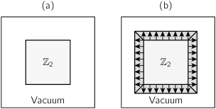
Figure 1: Identical samples cut from a strong $\mathbb{Z}_{2}$ topological insulator, but with two different surface preparations. (a) Time-reversal symmetry is preserved at vacuum-terminated surfaces; the net magnetoelectric coupling of this sample is zero. (b) Time-reversal symmetry is broken at the surface as a result of exchange coupling to an insulating ferromagnetic adlayer; if this opens a gap in the surface-state spectrum, the entire sample will behave as if it has a magnetoelectric coupling of exactly $\theta=\pi$.

Next we analyze the case of a strong $\mathbb{Z}_{2}$ topological insulator having $\theta=\pi$, or equivalently, ${\bm{\alpha}}={\bm{\alpha}}^{\rm CS}=(e^{2}/2h)\,\mathbf{I}$. We first consider a sample of such a system that has $T$ symmetry conserved at its surfaces, as in Fig. 1(a). Again, since the entire sample is $T$-symmetric, its experimentally measurable magnetoelectric coupling tensor $\bm{\beta}$ clearly has to vanish. Using Eq. (16) and the fact that $m$ can take on only integer, and not half-integer, values, we conclude that the only way to make the response of the entire sample vanish is to have $\Delta_{ij}$ be non-zero. This requires that the surfaces of such a system must be metallic. Moreover, since the contribution $\Delta_{ij}$ of the metallic surface band to the surface anomalous Hall conductivity is just given by the Berry phase around the Fermi loop,Haldane (2004) the needed cancellation requires this Berry phase to be exactly $\pm\pi$. All this is in precise accord with the known properties of $\mathbb{Z}_{2}$-odd insulators and their topologically protected surface states.Hasan and Kane (2010)

The Kramers degeneracy at the Dirac cone in the surface bandstructure can be removed by the application of a $T$-breaking perturbation to the surface. In principle, this could be accomplished, for example, by applying a local magnetic field to the surface or by interfacing the surface to an insulating magnetic overlayer. In the latter case, the interatomic exchange couplings provide a kind of effective magnetic field acting on the surface layer of the topological insulator. If the local Fermi level resides in the gap opened by field, then the surface becomes insulating. If the field can be consistently oriented (see Ref. Qi et al., 2008) on each patch of the surface, either along or opposite the direction of surface normal vector $\bf n$ (as shown in Fig. 1(b)), then the entire surface becomes insulating. It is important that the field is applied consistently in the same direction with respect to $\bf n$, since conducting channels will otherwise appear at domain boundaries.Hasan and Kane (2010)

If all of these requirements are met, the surface contribution $\Delta_{ij}$ to $\bm{\beta}$ vanishes, so that ${\bm{\beta}}={\cal V}{\bm{\alpha}}$ with $\bm{\alpha}$ given only by bulk value of $\theta=\pi$ (assuming $m=0$ for simplicity). Therefore such a sample of a strong $\mathbb{Z}_{2}$ topological insulator would behave as if the entire sample has exactly half a quantum of magnetoelectric coupling ($\theta=\pi$), even though its bulk is time-reversal symmetric!

II.4.2 Prospects for large-$\theta$ materials

Recently surface-sensitive ARPES measurements have experimentally confirmed that several compounds,Hsieh et al. (2008, 2009); Xia et al. (2008) including Bi_1-xSb_x, Bi₂Se₃, Bi₂Te₃ and Sb₂Te₃, do indeed behave as strong $\mathbb{Z}_{2}$ topological insulators. Therefore their bulk wavefunctions must be characterized by $\theta=\pi$. Up to now, the corresponding magnetoelectric response has not been measured experimentally, in part because of the difficulties in obtaining truly insulating behavior in the bulk, as well as the need to gap the surfaces by putting them in contact with magnetic overlayers as described earlier.

We believe that a more promising approach to observing a large CSOMP (i.e., $\theta$ comparable to $\pi$) is to consider an insulator that has neither $T$ nor spatial inversion symmetry. In this case the $\mathbb{Z}_{2}$ classification does not apply, and the surface can be gapped without any need to apply a $T$-breaking perturbation. (A more precise statement of the symmetry considerations will be given in Sec. II.5.) The sample can then display a bulk magnetoelectric coupling of the simple form ${\bm{\beta}}={\cal V}{\bm{\alpha}}$. We note that an orbital magnetoelectric coupling of $\theta\simeq\pi$ (i.e., $\alpha_{\rm r}\simeq 1/137$) would correspond to $\alpha^{\rm EH}\simeq 24.3$ ps/m, a value that is significantly larger than the observed coupling in Cr₂O₃, one of the best-studied magnetoelectric materials. For comparison, the reported experimental values for $\alpha^{\rm EH}_{\perp}$ in Cr₂O₃, which are presumably dominated by spin-lattice coupling, range between 0.7 and 1.6 ps/m at 4.2 K.Wiegelmann et al. (1994); Kita et al. (1979)

Of course, in order to have a good chance of finding a material with a large $\theta$, it may be advisable to look for materials with some of the same characteristics as the known $\mathbb{Z}_{2}$-odd insulators, of which the most important is probably the presence of heavy atoms with strong spin-orbit coupling. We see no strong reason why such a search might not reveal a material having a large OMP in the above sense.

Figure 2: (Color online) Schematic view of the allowable values of $\theta$ in different parts of the two-parameter space of some unspecified model Hamiltonian. Horizontal axis corresponds to the perturbation that preserves at least one of the symmetries that render $\theta$ to be $0$ or $\pi$ (see Sec. II.5). Vertical axis parameterizes a perturbation that breaks those symmetries and allows $\theta$ to be arbitrary. See text for the details.

To illustrate the kind of a search we have in mind, consider some model Hamiltonian that depends on two parameters, one that preserves either the $T$ or spatial inversion symmetry (or both), and another that that breaks symmetry such that $\theta$ takes a generic value. The possible behavior of such a model is sketched in Fig. 2, where these two parameters are plotted along the horizontal and vertical axes respectively. The figure also indicates the generic value of $\theta$ in each region of parameter space. Along the horizontal axis, where the extra symmetry is present, three regions are indicated. The black dot indicates a point of gap closure forming the boundary between a normal $T$-symmetric insulator regime on the left ($\theta=0$) and a strong $\mathbb{Z}_{2}$ topological insulator regime on the right ($\theta=\pi$). If the system is carried along the horizontal axis, $\theta$ must be either $0$ or $\pi$ except at the critical point, and it must therefore jump discontinuously when passing through this point of metallic behavior. On the other hand, if we now imagine passing from the $\mathbb{Z}_{2}$-odd to the $\mathbb{Z}_{2}$-even phase along the dashed curve in Fig. 2, $\theta$ can vary smoothly and continuously from $\pi$ to 0 without any gap closure anywhere along the path. If we can identify a material lying near, but not at, the right end of this dashed path, it could be the kind of large-$\theta$ material we seek.

Thus, our ultimate goal is to use first-principles calculations to search for a large $\theta$, not in a topological insulator, but in an “ordinary” (but presumably strongly spin-orbit coupled) insulating magnetic material. While our work has yet to result in the identification of a large-$\theta$ material of this kind, it represents a first step in the desired direction.

II.5 General symmetry considerations

Recall that $\theta$ is a pseudoscalar that changes sign under time-reversal and spatial-inversion symmetries (since $\bf B$ changes sign under $T$ while $\bm{{\mathcal{E}}}$ changes sign under inversion). On the other hand, $\theta$ is invariant under any translation or proper rotation of a crystal. Therefore if the magnetic point group of a crystal contains an element that involves $T$, possibly combined with a proper rotation, the value of $\theta$ is constrained to be $0$ or $\pi$ (modulo $2\pi$) as discussed earlier. The same happens if the magnetic point group contains inversion symmetry or any other improper rotation.

All 32 of the 122 magnetic point groups that do not contain such symmetry elements, and which therefore allow for an arbitrary value of $\theta$, are listed in Table 1. (The bold entries in the table are those magnetic groups for which the tensor ${\bm{\alpha}}$ must be isotropic, i.e., a constant times the identity matrix; the same magnetic groups were also analyzed in Ref. Hehl, F. W. et al., 2009). Clearly we can constrain our search for interesting materials to the cases listed in the Table.

Table 1: Magnetic point groups for which a non-zero CSOMP is allowed by symmetry. Notation follows Ref. Cracknell, 1975. Point groups in bold allow only for a purely isotropic magnetoelectric tensor.

$1$	$\bar{1}^{\prime}$	$2$	$m^{\prime}$	$2/m^{\prime}$	$222$	$m^{\prime}m^{\prime}2$
$m^{\prime}m^{\prime}m^{\prime}$	$4$	$\bar{4}^{\prime}$	$4/m^{\prime}$	$3$	$\bar{3}^{\prime}$	$6$
$\bar{6}^{\prime}$	$6/m^{\prime}$	$422$	$4m^{\prime}m^{\prime}$	$\bar{4}^{\prime}2m^{\prime}$	$4/m^{\prime}m^{\prime}m^{\prime}$	$32$
$3m^{\prime}$	$\bar{3}^{\prime}m^{\prime}$	$622$	$6m^{\prime}m^{\prime}$	$\bar{6}^{\prime}m^{\prime}2$	$6/m^{\prime}m^{\prime}m^{\prime}$
$\bf{23}$	$\bf{m^{\prime}3}$	$\bf{432}$	$\bf{\bar{4}^{\prime}3m^{\prime}}$	$\bf{m^{\prime}3m^{\prime}}$

III Methods

In this section we present our methods for calculating the CSOMP in the framework of density-functional theory, and analyze in more detail its mathematical properties and the formal similarities to the formulas used to calculate electric polarization and anomalous Hall conductivity.

III.1 Review of Berry formalism

Assume we are given the Bloch wavefunctions $|\psi_{n{\bf k}}\rangle=e^{i{\bf k}\cdot{\bf r}}|u_{n{\bf k}}\rangle$ as a function of wavevector ${\bf k}$ in the $d$-dimensional BZ ($d=1$, 2, or 3) for an insulator having valence bands indexed by $n\in\{1,\ldots,N\}$. We work with the cell-periodic Bloch functions $u_{n{\bf k}}({\bf r})=e^{-i{\bf k}\cdot{\bf r}}\psi_{n{\bf k}}({\bf r})$ and allow them to be mixed at each $k$ point by an arbitrary $k$-dependent unitary matrix

$$|u_{n{\bf k}}\rangle\rightarrow|u_{m{\bf k}}\rangle U_{mn{\bf k}}$$ (18)

(sum on $m$ implied). After this gauge transformation the wavefunctions are no longer eigenfunctions of the Hamiltonian, but they span the same $N$-dimensional subset of the Hilbert space as the true eigenfunctions. For any given choice of gauge, we define the Berry connection

$${\cal A}_{mn{\bf k}j}=\langle u_{m{\bf k}}|i\frac{\partial}{\partial k_{j}}|u_{n{\bf k}}\rangle,$$ (19)

which is a $k$-dependent $N\times N\times d$ matrix that measures, at each $k$ point, the infinitesimal phase difference between the $m$-th and $n$-th wavefunctions associated with neighboring points along Cartesian direction $j$ in $k$ space. This object was already briefly introduced in Eq. (8).

In the context of electronic structure calculations, we can now list three material properties that can be evaluated knowing only the Berry connection: the electric polarization, the intrinsic anomalous Hall conductivity, and the CSOMP.

The electric polarization $\cal P$ already appears in dimension $d=1$ and it can be evaluated as an integral of the Berry connection over the one-dimensional BZ as King-Smith and Vanderbilt (1993)

$${\cal P}=-\frac{e}{2\pi}\displaystyle\int_{\rm BZ}dk\,{\rm tr}{\cal A}_{k},$$ (20)

where the trace is performed over the band indices of the Berry connection, as in Eq. (10). The integrand is also referred to as the Chern-Simons 1-form, and its integral over the BZ is well known to be defined only modulo $2\pi$. Any periodic adiabatic evolution of the Hamiltonian ${\mathcal{H}}(\lambda)$ whose first Chern number in ($k,\lambda$) space is non-zero will change the integral above by a multiple of $2\pi$.King-Smith and Vanderbilt (1993)

Unlike one-dimensional systems, crystals in $d=2$ can have an anomalous Hall conductivity. For a metal, the intrinsic contribution from a band crossing the Fermi level can be evaluated as a line integralHaldane (2004); Wang et al. (2006)

$$\sigma^{\rm AH}=\frac{e^{2}}{h}\frac{1}{2\pi}\displaystyle\oint_{\rm FL}d{\bf k}\cdot{\bm{{\cal A}}}_{{\bf k}}$$ (21)

over the Fermi loop. Fully-filled deeper bands can also make a quantized contribution given by a similar integral, but around the entire BZ; this is the only contribution in the case of a quantum anomalous Hall insulator.Haldane (1988) (In both cases, the gauge choice on the boundary of the region should be consistent with a continuous, but not necessarily $k$-periodic, gauge in its interior; alternatively, each expression can be converted to an area integral of a Berry curvature to resolve any uncertainty about branch choice. See Ref. Wang et al., 2007 for more details.)

Finally, unlike one- or two-dimensional systems, three-dimensional systems can have an isotropic magnetoelectric coupling. The CSOMP can be evaluated in $d=3$ as a BZ integration of a quantity involving the Berry connection:

$$\theta=-\frac{1}{4\pi}\displaystyle\int_{\rm BZ}d^{3}k\epsilon_{ijk}{\rm tr}\left[{\cal A}_{i}\partial_{j}{\cal A}_{k}-\frac{2i}{3}{\cal A}_{i}{\cal A}_{j}{\cal A}_{k}\right].$$ (22)

The integrand in this expression is known as the Chern-Simons 3-form, and its integral over the entire BZ is again ill-defined modulo $2\pi$, since any periodic adiabatic evolution of the Hamiltonian ${\mathcal{H}}(\lambda)$ whose second Chern number in $({\bf k},\lambda)$ space is non-zero will change $\theta$ by an integer multiple of $2\pi$.Qi et al. (2008); Essin et al. (2009)

Figure 3: Graphical interpretation of Eqs. (20) (a), (21) (b) and (22) (c) in the case of one occupied electron band and for cubic crystal symmetry, for simplicity. See text for more detail.

The sketches in Fig. 3 compare the geometrical characters of the operations needed to evaluate Eqs. (20-22) in practice. We consider the case of one occupied electron band for simplicity. The polarization of Eq. (20) is calculated by a line integral; on a discrete $k$-mesh, the integral of the Berry connection ${\cal A}$ over each of line segment, as in Fig. 3(a), is converted to a discretized form (see Eq. (23)). Similarly, in two dimensions the anomalous Hall conductivity of Eq. (21) can be calculated as suggested in Fig. 3(b) by dividing the occupied part of the BZ into small square segments and then integrating ${\cal A}$ around each square. (Equivalently, one can integrate ${\cal A}$ along the Fermi loop.Wang et al. (2007)) In three dimensions, Fig. 3(c), Eq. (22) can be evaluated by dividing the BZ into small cubes. In each, one needs to multiply the integral of ${\cal A}$ along one of the Cartesian directions (as in Eq. (20)) with the integral of Berry connection in the square orthogonal to that direction (as in Eq. (21)), followed by a symmetrization over the three Cartesian directions.

III.2 Numerical evaluation of $\theta$

In electronic-structure calculations, the cell-periodic wavefunctions $|u_{n{\bf k}}\rangle$ are typically calculated on a uniform $k$-space grid with no special gauge choice; in general, one should assume that the phases have been randomly assigned. Nevertheless, it is straightforward to construct a gauge-invariant polarization formula that is immune to this kind of scrambling of the gauge.Marzari and Vanderbilt (1997) In one dimension with $k_{j}$ for $j\in\{1,\ldots,M\}$ (where $k_{M}$ is the periodic image of point $k_{1}$), the electronic polarization is calculated as

$$P=\frac{e}{2\pi}{\rm Im}\ln\det\left[M_{k_{1}k_{2}}M_{k_{2}k_{3}}...M_{k_{M-1}k_{M}}\right]$$ (23)

where the overlap matrix $M_{kk^{\prime}}$ is defined as

$$\left[M_{kk^{\prime}}\right]_{mn}=\langle u_{mk}|u_{nk^{\prime}}\rangle.$$ (24)

The reason for using Eq. (23) is that the determinant of the matrix $M_{k_{1}k_{2}}M_{k_{2}k_{3}}...M_{k_{M-1}k_{M}}$ is gauge-invariant under any transformation in the form of Eq. (18). Additionally, the implementation of Eq. (23) is numerically stable even when there are band crossings. A similar gauge-invariant discretization can also be used to calculate the anomalous Hall conductivity $\sigma^{\rm AH}$.Wang et al. (2007)

Unfortunately, except in the single-band (“Abelian”) case, we are unaware of any corresponding gauge-invariant discretized formula for the integral of the Chern-Simons 3-form. As a result, we have no prescription for computing the CSOMP that is exactly gauge-invariant for a given choice of $k$ mesh. This is a serious problem. Unlike the calculation of the polarization, which is straightforward even if the gauge is randomly scrambled at each mesh point, the calculation of the CSOMP requires that we first identify a reasonably smooth gauge on the discrete mesh.

The problem of finding a smooth gauge in ${\bf k}$ is essentially the same as that of finding well-localized Wannier functions. For this reason, we have adopted here the approach of first constructing a Wannier representation for the valence bands, and then using it to compute the CSOMP. In fact, starting from Eq. (22), we derive an expression that allows us to compute $\theta$ directly in the Wannier representation. Once we have well-localized Wannier functions, this guarantees smoothness of the gauge and avoids problems with band crossings. Admittedly, such a formula still depends on the gauge choice, meaning that different choices of Wannier functions will lead to slightly different results. However, this difference will vanish as one increases the density of the $k$-point mesh, since in the continuum limit the $k$-space expression for $\theta$ is gauge-invariant (modulo $2\pi$). More precisely, we expect the calculation of $\theta$ to converge once the inverse of the $k$-point mesh spacing becomes much larger than the spread of the Wannier functions.

Therefore, we adopt the strategy of calculating $\theta$ on $k$ meshes of different density, and extrapolating $\theta$ to the limit of an infinitely dense mesh. Furthermore, we construct maximally-localized Wannier functions (MLWF) following Ref. Marzari and Vanderbilt, 1997, expecting this to give relatively rapid convergence as a function of the $k$ mesh density.

Recall that the Wannier function associated with (generalized) band index $n$ in unit cell ${\bf R}$ is defined in terms of the rotated Bloch states (18) as

$$|{\bf R}n\rangle=\frac{\Omega}{(2\pi)^{3}}\int d^{3}k\,e^{i{\bf k}\cdot({\bf r}-{\bf R})}|u_{m{\bf k}}\rangle U_{mn{\bf k}}.$$ (25)

In the case of MLWFs, the $U_{mn{\bf k}}$ are chosen in such a way that the total quadratic spread of the Wannier function is minimized.Marzari and Vanderbilt (1997) (In practice the BZ integral is replaced by a summation over a uniform grid of $k$ points.)

Using Eq. (25), one can relate the Berry-connection matrix ${\cal A}_{mn{\bf k}j}$ in the smooth gauge to the Wannier matrix elements of the position operator throughMarzari and Vanderbilt (1997)

$$A_{mn{\bf k}j}=\sum_{{\bf R}}e^{i{\bf k}\cdot{\bf R}}\langle{\bf 0}m|r_{j}|{\bf R}n\rangle.$$ (26)

Replacing each occurrence of $A_{j}$ in Eq. (22) with the above gives, after some algebra,

$$\theta= \frac{1}{4\pi}\frac{(2\pi)^{3}}{\Omega}\epsilon_{ijk}{\rm Im}\bigg{[}\frac{1}{3}\sum_{\bf R}\langle{\bf 0}m|r_{i}|{\bf R}n\rangle\langle{\bf R}n|r_{j}|{\bf 0}m\rangle R_{k}$$

$$-\frac{2}{3}\sum_{{\bf R}{\bf P}}\langle{\bf 0}l|r_{i}|{\bf R}m\rangle\langle{\bf R}m|r_{j}|{\bf P}n\rangle\langle{\bf P}n|r_{k}|{\bf 0}l\rangle\bigg{]},$$ (27)

where the sum is implied over band ($lmn$) and Cartesian ($ijk$) indices.

To obtain a more symmetric form, we introduce a modified position-operator matrix element between WFs defined as

$$\langle{\bf R}m|\tilde{r}_{i}|{\bf P}n\rangle=\langle{\bf R}m|r_{i}|{\bf P}n\rangle\left(1-\delta_{mn}\delta_{{\bf R}{\bf P}}\right)$$ (28)

and a notation for the Wannier center

$$\tau_{ni}=\langle{\bf 0}n|r_{i}|{\bf 0}n\rangle.$$ (29)

Then Eq. (27) becomes

$$\theta= \frac{1}{4\pi}\frac{(2\pi)^{3}}{\Omega}\epsilon_{ijk}\;\times$$ (30)

$$\;{\rm Im}\bigg{[}\sum_{\bf R}\langle{\bf 0}m|\tilde{r}_{i}|{\bf R}n\rangle\langle{\bf R}n|\tilde{r}_{j}|{\bf 0}m\rangle\left(R_{k}+\tau_{nk}-\tau_{mk}\right)$$

$$\;-\sum_{{\bf R}{\bf P}}\frac{2}{3}\langle{\bf 0}l|\tilde{r}_{i}|{\bf R}m\rangle\langle{\bf R}m|\tilde{r}_{j}|{\bf P}n\rangle\langle{\bf P}n|\tilde{r}_{k}|{\bf 0}l\rangle\bigg{]}.$$ (31)

We find this form more convenient because it separates the contributions of diagonal and off-diagonal elements of position operators. (It is also manifestly invariant to the reassignment of a Wannier function to a neighboring cell.) The validity of Eqs. (27) and (31) has been tested numerically by comparing with the evaluation of Eq. (22) for the case of a tight-binding model introduced in Ref. Malashevich et al., 2010. The evaluated expressions agreed to numerical accuracy after extrapolation to the infinitely dense mesh. These expressions can also be shown to be gauge-invariant by working directly within the Wannier representation.

III.3 Computational details

Calculations of the electronic ground state and of structural relaxations were performed using the Quantum-ESPRESSO package,Giannozzi et al. (2009) and the Wannier90 codeMostofi et al. (2008) was used for constructing maximally localized Wannier functions. We used radial-grid discretized HGHHartwigsen et al. (1998) norm-conserving pseudopotentials. Calculations were performed in the noncollinear spin framework, including spin-orbit effects as incorporated in the pseudopotentials. In all calculations we used the Perdew-WangPerdew and Wang (1992) LDA energy functional. The pseudopotentials used for Cr, Fe and Gd contain semi-core states, while the ones for Al, Bi, Se and O do not.

The self-consistent calculations on Cr₂O₃ were performed on a $4\times 4\times 4$ Monkhorst-PackMonkhorst and Pack (1976) grid in $k$ space. Non-self-consistent calculations for the Wannier-function construction were performed on $k$-space grids containing the origin and ranging in size from $6\times 6\times 6$ to $12\times 12\times 12$. The plane-wave energy cutoff was chosen to be 150 Ry.

In the case of Bi₂Se₃, the self-consistent calculations were performed on a $6\times 6\times 6$ grid with energy cutoff of 60 Ry, while the non-selfconsistent calculation was done on grids between $6\times 6\times 6$ and $11\times 11\times 11$.

The position-operator matrix elements $\langle{\bf 0}m|r_{j}|{\bf R}n\rangle$ needed to evaluate Eq. (31) were calculated in $k$ space by inverting the Fourier sum in Eq. (26) over the non-self-consistent $k$-point mesh, and then approximating the $k$ derivative in Eq. (19) by finite differences on that mesh, as detailed in Ref. Wang et al., 2006.

IV Results and discussion

IV.1 Conventional magnetoelectrics

In this section we present the results of our first-principles electronic-structure calculations of $\theta$. We begin with conventional magnetoelectrics, i.e., materials that are already experimentally known to have a non-zero magnetoelectric tensor. Some of these materials do not allow all diagonal components of the magnetoelectric tensor to be non-zero. We omit those materials from our analysis here, since we are interested in calculating the CSOMP part of the magnetoelectric coupling, which would vanish in such cases. We first present our results on Cr₂O₃ in some detail, and then briefly discuss our results for BiFeO₃ and GdAlO₃.

IV.1.1 Calculation of $\theta$ in Cr₂O₃

Figure 4: (Color online) (a) Rhombohedral unit cell of Cr₂O₃. Magnetic moments on Cr atoms are indicated by red arrows and oxygen octahedra are drawn around each Cr atom. (b) Schematic of hexagonal unit cell of Bi₂Se₃ with imposed local Zeeman field on Bi atoms. Induced magnetic moments are shown by red arrows. Thick blue lines indicate Se layers; letters (ABC) indicate stacking sequence. In both panels, the vertical line indicates the 3-fold rhombohedral axis, and the cross designates a 2-fold rotation axis orthogonal to the plane of the figure (also a center of inversion coupled with time reversal).

We first fully relax the structure in the R$\bar{3}$c space group and obtain the Wyckoff position to be $x=0.1575$ for Cr atoms (4c orbit) and $x=-0.0690$ for O (6e orbit). The length of the rhombohedral lattice vector is $a=5.3221$ Å while the rhombohedral angle is $53.01^{\circ}$. The Cr atoms have magnetic moments pointing along the rhombohedral axis as illustrated in Fig. 4(a) in an antiferromagnetic arrangement. The value of the magnetic moment is 2.0 $\mu_{\rm B}$ per Cr atom and the electronic gap is 1.3 eV, which agrees well with previous LDA+U calculationsMosey and Carter (2007); Shi et al. (2009) in the limit where the on-site Coulomb parameter $U$ is set to zero.

Neglecting for a moment the magnetic spins on the Cr sites, the space-group generators are a three-fold rotation, a two-fold rotation, and an inversion symmetry as indicated in Fig. 4(a). Its point group is therefore $\bar{3}m$. If we now include the spins on the Cr atoms in the analysis, we find that the three-fold and two-fold rotations remain, while the inversion becomes a symmetry only when combined with time-reversal. Therefore the magnetic point group of Cr₂O₃ is $\bar{3}^{\prime}m^{\prime}$. This magnetic point group allows $\theta$ to be different from $0$ or $\pi$, as discussed in Sec. II.5.

Figure 5: (Color online) Calculated value of $\theta$ in Cr₂O₃ for varying densities of $k$-space grids, where $\Delta k$ is the nearest-neighbor distance on the grid. Top axis specifies the size of the corresponding uniform Monkhorst-Pack grid. Line indicates a quadratic extrapolation of $\theta$ to the infinitely dense $k$ mesh.

Figure 5 shows the calculated values of $\theta$ using Eq. (31) for Cr₂O₃ with $k$-space meshes of various densities. The line indicates the second-order polynomial extrapolation to an infinitely dense mesh. The extrapolated value of $\theta$ is $1.3\times 10^{-3}$, which is a small fraction of the quantum of OMP $\theta=2\pi$ and corresponds to $\alpha^{\rm EH}_{xx}=\alpha^{\rm EH}_{yy}=\alpha^{\rm EH}_{zz}=0.01$ ps/m. The positive sign of $\theta$ pertains to the pattern of Cr magnetic moments shown in Fig. 4(a); reversal of all magnetic moments would flip the sign of $\theta$.

In order to compare this value of the magnetoelectric coupling with experimental values and other theoretical calculations, we somewhat arbitrarily define

$$\alpha^{\rm eff}=\frac{|\alpha_{xx}|+|\alpha_{yy}|+|\alpha_{zz}|}{3}.$$ (32)

The value of $\alpha^{\rm eff}$ obtained from the results of Ref. Delaney et al., 2009 is $0.23$ ps/m for the purely electronic part of the spin-mediated component. Therefore, our calculated CSOMP contribution in Cr₂O₃ amounts to only 4% of this electronic spin component. The ionic component of the spin response calculated by the same authors results in $\alpha^{\rm eff}=0.74$ ps/m, while the one calculated in Ref. Íñiguez, 2008 is about 2.6 times smaller, $0.29$ ps/m. (In both of these calculations, $\alpha_{zz}$ is zero.) Finally, experimental measurements of the magnetoelectric tensor in Cr₂O₃ at 4.2 K vary between $\alpha^{\rm eff}=0.55$ ps/m and $1.17$ ps/m (see Refs. Wiegelmann et al., 1994 and Kita et al., 1979 respectively).

Clearly, our computed CSOMP contribution for Cr₂O₃ is negligible, being two orders of magnitude smaller than the dominant lattice-mediated spin contribution. This is probably not surprising, since the spin-orbit coupling is relatively weak in this material. Given that it is weak, we can guess that that magnitude of the CSOMP should be linear in the strength of the spin-orbit interaction in Cr₂O₃. Our calculations allow us to check this by varying the spin-orbit interaction strength $\lambda_{\rm SO}$ between $0$ (no spin orbit) and $1$ (full spin-orbit interaction). As shown in Fig. 6, if we calculate $\theta$ for various intermediate values of $\lambda_{\rm SO}$, we see that the CSOMP does indeed depend roughly linearly on $\lambda_{\rm SO}$.

Figure 6: (Color online) Calculated $\theta$ in Cr₂O₃ as a function of spin-orbit coupling strength, scaled such that $\lambda_{\rm SO}=1$ corresponds to the full spin-orbit coupling strength and $\theta_{0}=\theta(\lambda_{\rm SO}=1)$.

IV.1.2 Other conventional magnetoelectrics

We have also carried out calculations of $\theta$ in BiFeO₃ and GdAlO₃, but with a smaller number of $k$-point grids than in the case of Cr₂O₃. Therefore, our results are less accurate, but should still give a correct order-of-magnitude estimate of $\theta$.

For BiFeO₃ we perform the calculation in the 10-atom antiferromagnetic unit cell (the long-wavelength spin spiral was suppressed). We obtain an electronic band gap of 0.95 eV with magnetic moments of 3.5 $\mu_{\rm B}$ on each Fe atom, and with a net magnetization of 0.1 $\mu_{\rm B}$ per 10-atom primitive unit cell due to the canting of the Fe magnetic moments. Extrapolating $\theta$ to an infinitely dense mesh using just $6\times 6\times 6$ and $8\times 8\times 8$ $k$-point meshes, we obtain $\theta=0.9\times 10^{-4}$. In the case of GdAlO₃ we calculate the electronic band gap to be 5.0 eV and the Gd magnetic moment to be 6.7 $\mu_{\rm B}$. We obtain a value of $\theta=1.1\times 10^{-4}$ after extrapolating calculations using $4\times 4\times 4$ and $6\times 6\times 6$ $k$-space meshes. Thus, it is clear that the CSOMP is very small in both materials.

IV.2 Strong $\mathbb{Z}_{2}$ topological insulators

We now investigate the CSOMP in the case of Bi₂Se₃, which is known experimentallyXia et al. (2008) and theoreticallyZhang et al. (2008) to belong to the class of strong $\mathbb{Z}_{2}$ topological insulators. In the absence of broken $T$ symmetry, such a material should have a $\theta$ of exactly $\pi$ (modulo $2\pi$). We first confirm this numerically. Then, in Sec. IV.3, we also study what happens when $T$ is broken artificially by inducing antiferromagnetic order on the Bi atoms and tracking the resulting variation of $\theta$.

Bi₂Se₃ is known to belong to space group R$\bar{3}$m, with Bi at a 2c site and Se at the high-symmetry 1a site as well as at a 2c site. In our calculations we find that the Wyckoff parameters for Bi and Se are $x=0.4013$ and $0.2085$ respectively. We also find the length of the rhombohedral lattice vector to be $a=9.5677$ Å and the rhombohedral angle to be only $24.77^{\circ}$. The electronic gap is calculated to be 0.4 eV.

The generators of the R$\bar{3}$m space group are again three-fold and two-fold rotations and inversion (point group $\bar{3}m$). Since the system is nonmagnetic, the magnetic space group also contains the $T$ symmetry operator, and its magnetic point group is $\bar{3}m1^{\prime}$. According to the analysis given in Sec. II.5, it is clear that $\theta$ must therefore be zero or $\pi$ (modulo $2\pi$).

Since we know that Bi₂Se₃ is a strong $\mathbb{Z}_{2}$ topological insulator, we expect that $\theta$ should be equal to $\pi$ (modulo $2\pi$). However, special care needs to be taken in order to evaluate $\theta$ in such a case, because the choice of a smooth gauge becomes problematic. Specifically, it is known that the $\mathbb{Z}_{2}$ topology presents an obstruction to the construction of a Wannier representation (or equivalently, a smooth gauge in $k$ space) that respects $T$ symmetry.Fu and Kane (2006); Roy (2009a) Therefore, during the maximal localization procedure, one needs to choose trial Wannier functions that do not take the form of Kramers pairs, thereby explicitly breaking the $T$ symmetry.Soluyanov and Vanderbilt (2010) (It is important to note that this choice of Wannier functions does not bias our calculation towards having $\theta=\pi$, since the same starting choice of $T$-symmetry-broken Wannier functions for a normal $T$-symmetric insulator would result in $\theta=0$ up to the numerical accuracy of the calculation.)

Figure 7: (Color online) Calculated value of $\theta$ in Bi₂Se₃ for varying densities of $k$-space grids, where $\Delta k$ is the nearest-neighbor distance on the grid. Top axis specifies the size of the corresponding uniform Monkhorst-Pack grid. Line indicates a quadratic extrapolation of $\theta$ to the infinitely dense $k$ mesh.

Our results for $\theta$ in Bi₂Se₃ are given in Fig. 7 for various densities of $k$ meshes, ranging from $6\times 6\times 6$ to $11\times 11\times 11$. A quadratic polynomial extrapolation to the infinitely dense mesh limit gives $\theta=1.07\pi$. This is in reasonable agreement with the expected value of $\theta=\pi$, given the uncertainties in the extrapolation. (Of course, if we make a time-reversed choice of starting Wannier functions, we obtain $\theta=-1.07\pi$, which is consistent, within the errors, with $\theta=-\pi$ and modulo $2\pi$ to $\theta=\pi$.) Clearly the convergence with respect to mesh density is somewhat slow, making a precise extrapolation difficult. The reasons for this, and some possible paths to improvement, will be discussed in Sec. V.

IV.3 $\mathbb{Z}_{2}$-derived nontopological insulators with broken symmetries

Even though $\theta=\pi$ in Bi₂Se₃, a finite sample with $T$ symmetry preserved everywhere, including at the surfaces, will not exhibit any magnetoelectric coupling. From the point of view of the discussion in Sec. II.4, this happens because of an exact cancellation between $\theta=\pm\pi$ contributions coming from the bulk ($\alpha$) and metallic surface ($\Delta$) terms in Eq. (16). However, if one breaks the $T$ symmetry in the bulk (and possibly some other bulk symmetries, as detailed in Sec. II.5), the CSOMP term can become allowed.

The magnetic space group of Bi₂Se₃ contains both $T$ and spatial inversion symmetries. The presence of either by itself is enough to insure that $\theta=0$ or $\pi$ (modulo $2\pi)$. Now let us consider turning on, “by hand,” a local Zeeman field on each Bi atom in the staggered arrangement shown in Fig. 4(b), i.e., with fields oriented parallel to the rhombohedral axis and alternating in sign. The induced magnetic moments along the three-fold axis preserve both three-fold and two-fold rotation symmetries; both inversion and $T$ symmetries are broken, but $T$ taken together with inversion is still a symmetry. The resulting magnetic point group of the system is again $\bar{3}^{\prime}m^{\prime}$, as it was for Cr₂O₃, and it does allow for a CSOMP (the same magnetic arrangement has also been discussed in Ref. Li et al., 2010 in a different context).

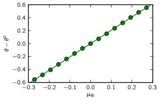
Figure 8: Calculated value of $\theta$ (vertical axis) and induced magnetic moment on the Bi atom (horizontal axis) for Bi₂Se₃ with artificially applied staggered Zeeman field on Bi atoms, as described in the text. $\theta^{0}$ is the value of CSOMP when magnetic field is not present.

In the density functional calculation one can easily apply a local Zeeman field to individual atoms in an arbitrary direction. Using this method, we have calculated the CSOMP in Bi₂Se₃ with the pattern of local fields described previously and illustrated in Fig. 4(b). Fig. 8 presents the calculated values of $\theta$ as a function of induced magnetic moment on Bi, where a positive $\mu_{\rm Bi}$ corresponds to the pattern of magnetic moments indicated in Fig. 4(b). (Actually this was done by applying the full extrapolation procedure of Fig. 7 for one case, $\mu_{\rm Bi}=0.16\,\mu_{\rm B}$, and using this to scale the results calculated on the $10\times 10\times 10$ grid at other $\mu_{\rm Bi}$.) The dependence of the change in CSOMP on the magnetic moment is linear over a wide range. One can see that for a relatively moderate magnetic moment of $\pm$0.27 $\mu_{\rm B}$, the value of $\theta$ is changed from $\pi$ to $\pi\pm$0.55. (For much higher local magnetic fields, Bi₂Se₃ becomes metallic and the CSOMP becomes ill-defined.)

These results indicate that it is possible, at least in principle, for a magnetic material to have a large but unquantized value of $\theta$, thereby providing an incentive for future searches for materials in which such a state arises spontaneously, without the need to apply perturbations by hand as done here.

V Summary and outlook

In this manuscript, we have presented a first-principles method for calculating the Chern-Simons orbital magnetoelectric coupling in the framework of density-functional theory. We have also carried out calculations of this coupling for a few well-known magnetoelectric materials, namely Cr₂O₃, BiFeO₃ and GdAlO₃. Unfortunately, in these materials the CSOMP contribution to the total magnetoelectric coupling is quite small. This is not surprising, since in most magnetoelectric materials the coupling is expected to be dominated by the lattice-mediated response, whereas the CSOMP is a purely electronic (frozen-ion) contribution. Moreover, the CSOMP is part of the orbital frozen-ion response, which is again expected to be smaller then the spin response, except perhaps in systems with very strong spin-orbit coupling, as discussed in Sec. I. For example, in Cr₂O₃ the CSOMP is about 4% of the frozen-ion spin contribution to the magnetoelectric coupling.

On the other hand, we have reasons to believe that in special cases the CSOMP contribution to the magnetoelectric coupling could be large compared to the total magnetoelectric coupling in known magnetoelectrics such as Cr₂O₃. After all, as already pointed out in Sec. II.4.2, $\mathbb{Z}_{2}$ topological insulators are predicted to display a large magnetoelectric effect of purely orbital origin when their surfaces are gapped in an appropriate way. If this is so, why shouldn’t a similar effect occur in certain $T$-broken systems?

As a proof of concept for the existence of those special cases, we have considered Bi₂Se₃ with inversion and time-reversal symmetries explicitly broken “by hand.” Here we find that with a relatively modest induced magnetic moment on the Bi atoms, one can still achieve quite a large change in the CSOMP.

On the computational side, there still remain several challenges. For example, the convergence of our calculations of the CSOMP with respect to the $k$-point mesh density is disappointingly slow. A direct calculation of $\theta$ in Bi₂Se₃ using a very dense mesh of $11\times 11\times 11$ $k$ points only manages to recover about 30% of the converged value of $\theta=\pi$, and an extrapolation procedure is needed to brings us within 10% of that value. This clearly points to the need for methodological improvements, and we now comment briefly on some possible paths for future work.

The slow convergence that we observe is related in part to the way in which we evaluate the position-operator matrix elements $\langle{\bf 0}m|r_{j}|{\bf R}n\rangle$. As discussed in Ref. Wang et al., 2006, the $k$-space procedure we adopted (see Sec. III.3) entails an error of ${\cal O}(\Delta k^{2})$. Preliminary tests on a tight-binding model suggest that an exponentially fast convergence of $\theta$ can be achieved by an alternative procedure, in which the WFs are first constructed on a real-space grid over a supercell (whose size scales with the $k$-mesh density), and the position matrix elements are then evaluated directly on that grid, as in Ref. Stengel and Spaldin, 2006. It may also be possible to improve the $k$-space calculation by using higher-order finite-difference formulas that have a more rapid convergence with respect to mesh density.

An alternative approach would be to develop a formula for the CSOMP that is exactly gauge invariant in the case of a discretized $k$-space grid. Such an expression already exists for the case of electronic polarization, Eq. (23), but we are aware of no counterpart for the CSOMP. Even though such an approach would not necessarily provide much faster convergence with respect to the $k$-space sampling, it would still be a significant improvement. For example, one would not need to construct a smooth gauge in $k$ space, which is a particular problem in the case of $\mathbb{Z}_{2}$ insulators (or for a symmetry-broken insulator in the vicinity of a $\mathbb{Z}_{2}$ phase). Another use of such a formula would be to calculate with relative ease the $\mathbb{Z}_{2}$ index of any insulator, even in the cases when other methodsFu et al. (2007); Moore and Balents (2007); Roy (2009b) cannot be applied (for example, when inversion symmetry is not present).

Furthermore, a full calculation of the electronic contribution to the orbital magnetoelectric response should also include the remaining two contributions given in Eqs. (6) and (7). This calculation would also require a knowledge of the first derivatives of the electronic wavefunctions with respect to electric field. While these derivatives are available as part of the linear-response capabilities of the Quantum-ESPRESSO package,Giannozzi et al. (2009) some care is needed to arrive at a robust implementation of Eqs. (6) and (7), as will be reported in a future communication.

Finally, recall that our calculations have all been carried out in the context of ordinary density-functional theory. In cases where orbital currents play a role, it is possible that current-density functionalsVignale and Rasolt (1988); Vignale (2004) could give an improved description. However, such functionals are still in an early stage of development and testing, and we prefer to focus first on exploring the extent to which conventional density functionals can reproduce experimental properties of systems in which orbital currents are present.

Overall, significant progress has been made in the ability to calculate the magnetoelectric coupling of real materials in the context of density-functional theory. The methods described in Ref. Íñiguez, 2008 and Delaney et al., 2009 allow for the calculation of both the electronic and lattice components of the spin (i.e., Zeeman) contribution to the magnetoelectric coupling. In principle at least, the lattice component of the orbital contribution could be computed using the methods of Ref. Ceresoli et al., 2006, while the remaining orbital electronic contributions can be computed from the formulas derived in Refs. Essin et al., 2010 and Malashevich et al., 2010 following the developments discussed here. We thus expect that the computation of all of the various contributions to the magnetoelectric coupling will soon be accessible to modern density-functional methods.