Spectral properties of two-body random matrix ensembles for boson systems with spin

Abstract

For $m$ number of bosons, carrying spin (${\bf s}=\frac{1}{2}$) degree of freedom, in $\Omega$ number of single particle orbitals, each doubly degenerate, we introduce and analyze embedded Gaussian orthogonal ensemble of random matrices generated by random two-body interactions that are spin ($S$) scalar [BEGOE(2)-${\bf s}$]. Embedding algebra for the BEGOE(2)-${\bf s}$ ensemble and also for BEGOE(1+2)-${\bf s}$ that includes the mean-field one-body part is $U(2\Omega)\supset U(\Omega)\otimes SU(2)$ with $SU(2)$ generating spin. A method for constructing the ensembles in fixed-($m,S$) spaces has been developed. Numerical calculations show that for BEGOE(2)-${\bf s}$, the fixed-$(m,S)$ density of states is close to Gaussian and level fluctuations follow GOE in the dense limit. For BEGOE(1+2)-${\bf s}$, generically there is Poisson to GOE transition in level fluctuations as the interaction strength (measured in the units of the average spacing of the single particle levels defining the mean-field) is increased. The interaction strength needed for the onset of the transition is found to decrease with increasing $S$. Propagation formulas for the fixed-$(m,S)$ space energy centroids and spectral variances are derived for a general one plus two-body Hamiltonian preserving spin. Derived also is the formula for the variance propagator for the fixed-$(m,S)$ ensemble averaged spectral variances. Using these, covariances in energy centroids and spectral variances are analyzed. Variance propagator clearly shows, by applying the Jacquod and Stone prescription, that the BEGOE(2)-${\bf s}$ ensemble generates ground states with spin $S=S_{max}$. This is further corroborated by analyzing the structure of the ground states in the presence of the exchange interaction $\hat{S}^{2}$ in BEGOE(1+2)-${\bf s}$. Natural spin ordering ($S_{max}$, $S_{max}-1$, $S_{max}-2$, $\ldots$, $0$ or $\frac{1}{2}$) is also observed with random interactions. Going beyond these, we also introduce pairing symmetry in the space defined by BEGOE(2)-${\bf s}$. Expectation values of the pairing Hamiltonian show that random interactions exhibit pairing correlations in the ground state region.

I Introduction

Random matrix theory has been established to be one of the central themes for chaotic quantum systems Ha-10 . The classical Gaussian orthogonal (GOE), unitary (GUE) and symplectic (GSE) ensembles of random matrices are ensembles of multi-body, not two-body interactions. However, finite interacting quantum systems, such as nuclei, atoms, quantum dots, small metallic grains and interacting spin systems modeling quantum computing core and BEC, are governed largely by two-body interactions and hence, it is important to consider ensembles generated by random two-body interactions. These ensembles are defined by representing the two-particle Hamiltonian by one of the classical ensembles (GOE, GUE, GSE) and then the many particle ($m>2$) Hamiltonian is generated by exploiting the direct product structure of the $m$-particle Hilbert spaces. As a random matrix ensemble in the two-particle spaces is embedded in the many particle Hamiltonian, these ensembles are generically called embedded ensembles (EE) and with GOE embedding, they will be EGOE’s. A wide variety of EE for fermions have been introduced in literature Fr-70 ; Bo-71 ; MF-75 ; Ko-01 ; Ma-10 ; Go-10 .

Simplest of EE is the embedded Gaussian orthogonal ensemble for spinless fermion systems generated by random two-body interactions, denoted by EGOE(2). In general, it is also possible to define EGOE($k$) ensembles generated by $k$-body ($k<m$) interactions MF-75 . It is useful to mention that many diversified methods like numerical Monte-Carlo methods, binary correlation approximation, trace propagation, group theory, supersymmetry and perturbation theory are used to derive generic properties of EE MF-75 ; Be-01 ; Ko-05 ; Ko-07 ; Ma-10b . Some of the generic results for EGOE($k$) are as follows: (i) eigenvalue density exhibits, with increasing $m$, transition from semicircle to Gaussian with $m=2k$ being the transition point Be-01 ; (ii) numerical studies have shown that the level and strength fluctuations follow GOE Br-81 ; (iii) there is average-fluctuation separation with increasing $m$ Br-81 ; Le-08 ; (iv) ensemble averaged transition strength densities follow bivariate Gaussian form and consequently, transition strength sums will be close to a ratio of two Gaussians FKPT ; and (v) there will be non-zero correlations between states with different particle numbers PW-07 ; Ko-06 . Besides two-body interactions, Hamiltonians for realistic systems contain a mean-field part [defined by non-degenerate single particle (sp) levels] and then the ensemble is denoted by EE(1+2). This ensemble exhibits, with increasing strength $\lambda$ of the interaction ($\lambda$ is in units of the average sp level spacing), three chaos markers defining transitions in level fluctuations ($\lambda_{c}$), strength functions ($\lambda_{F}$) and entropy ($\lambda_{d}$) respectively. Generic results of EE(2) are valid for EE(1+2) in the strong coupling regime ($\lambda>>\lambda_{F}$). Realistic systems also preserve various symmetries. For example, spin $S$ is a good quantum number for atoms and quantum dots, angular momentum $J$ and parity $\pi$ are good quantum numbers for nuclei and so on. Therefore, it is more appropriate to study EE with good symmetries. A simple but non-trivial extension of EE is to consider finite quantum systems with spin (${\bf s}=\frac{1}{2}$) and then the ensembles are called EE(1+2)-${\bf s}$. For finite interacting fermion systems, EGOE(1+2)-${\bf s}$ has been studied in detail using a mixture of numerical and analytical techniques Ko-06a ; Ma-09 ; Ma-10 and EGUE(2)-${\bf s}$ using Wigner-Racah algebra Ko-07 . Moreover, EGUE(2) with spin-isospin $SU(4)$ symmetry, comparatively complicated than the random matrix models analyzed before, has been recently introduced and analyzed in some detail Ma-10b . More importantly, there are now several applications of EE to mesoscopic systems Meso1 ; Meso2 ; JS-01 ; Ma-10c , quantum information science Br-08 and in investigating thermalization in finite quantum systems Ri-09 ; Sa-10 ; Sa-10a ; Ol-09 . Unlike for fermion systems, there are only a few EE investigations for finite interacting boson systems PDPK ; Ag-01 ; Ag-02 ; Ch-03 ; Ch-04 ; the corresponding EE are called BEE (B stands for bosons). Briefly, these studies are as follows.

Firstly, it is important to mention that, unlike fermion systems, for interacting spinless boson systems with $m$ bosons in $N$ sp orbitals, dense limit defined by $m\to\infty$, $N\to\infty$ and $m/N\to\infty$ is also possible as $m$ can be greater than $N$ for bosons. It is now well understood that BEGOE(2) [also BEGUE(2)] generates in the dense limit, eigenvalue density close to a Gaussian KP-80 ; PDPK . Also the ergodic property is found to be valid in the dense limit with sufficiently large $N$ Ch-03 ; there are deviations for small $N$ Ag-01 . Similarly, for BEGOE(1+2), as the strength $\lambda$ of the two-body interaction increases, there is Poisson to GOE transition in level fluctuations at $\lambda=\lambda_{c}$ Ch-03 and with further increase in $\lambda$, there is Breit-Wigner to Gaussian transition in strength functions Ch-04 . For BEGUE($k$), exact analytical results for the lowest two moments of the two-point function have been derived by Agasa et al Ag-02 . Level fluctuations and wavefunction structure in interacting boson systems are also studied using interacting boson models of atomic nuclei Al-91 ; Al-93 ; Ca-00 and a symmetrized two coupled rotors model Bo-98a ; Bo-98b . In addition, using random interactions in interacting boson models, there are several studies on the generation of regular structures in boson systems with random interactions Ku-97 ; BF-00 ; Ko-04 ; Yo-09 . Finally, there are also studies on thermalization in finite quantum systems using boson systems Ri-09 ; Sa-10 ; Sa-10a ; Ol-09 .

Going beyond the embedded ensembles for spinless boson systems, our purpose in this paper is to introduce and analyze spectral properties of embedded Gaussian orthogonal ensemble of random matrices for boson systems with spin degree of freedom [BEGOE(2)-${\bf s}$ and also BEGOE(1+2)-${\bf s}$] and for Hamiltonians that conserve the total spin of the $m$-boson systems. Here the spin is, for example, as the $F$-spin in the proton-neutron interacting boson model ($pn$IBM) of atomic nuclei Ca-05 . Just as the earlier embedded ensemble studies Ag-01 ; Ag-02 ; Ch-03 ; Ch-04 , a major motivation for the study undertaken in the present paper is its possible applications to ultracold atoms. There are several studies of the properties of a mixture of two species of atoms which correspond to pseudospin-$\frac{1}{2}$ bosons (i.e. two-component boson systems) with $m_{\bf s}=\pm\frac{1}{2}$ distinguishing the two species; see for example Al-03 ; Yu-10 . However, the Hamiltonians appropriate for these studies do not conserve the total spin (as the system does not have true $\frac{1}{2}$-spins) and therefore, the model study presented in the present paper will not be directly applicable to these systems in understanding their statistical properties. Nevertheless, the BEGOE(1+2)-${\bf s}$ with spin-$\frac{1}{2}$ bosons is a simple yet non-trivial extension of the spinless BEE. This ensemble is useful in obtaining several physical conclusions, like spin dependence of the order to chaos transition marker in level fluctuations, the spin of the ground state (gs), the spin ordering of excited states and pairing correlations in the gs region generated by random interactions, that explicitly require inclusion of spin degree of freedom (these are discussed in Sections III, V and VI). It should be emphasized that the present paper opens a new direction in defining and analyzing embedded ensembles for boson systems with symmetries. It is important to mention here that there are now many studies of spinor BEC using Hamiltonians conserving the total spin with the bosons carrying ${\bf s}=1$ (also higher) degree of freedom Pe-10 ; Yi-07 . Extensions of BEGOE(1+2)-${\bf s}$ with ${\bf s}=\frac{1}{2}$ to boson ensembles with integer spin ${\bf s}=1$ (or higher) is for future. Now we will give a preview.

In Section II, introduced is the new embedded ensemble BEGOE(2)-${\bf s}$ [and also BEGOE(1+2)-${\bf s}$] for a system of $m$ bosons in $\Omega$ number of sp orbitals that are doubly degenerate with total spin $S$ being a good symmetry. A method for the numerical construction of this ensemble in fixed-$(m,S)$ spaces is described. Numerical results for the ensemble averaged eigenvalue density, nearest neighbor spacing distribution and the long-range rigidity measure $\overline{\Delta}_{3}$ are presented in Section III. Propagation formulas for fixed-$(m,S)$ energy centroids and spectral variances for general one plus two-body Hamiltonians that preserve $S$ are given in Section IV. Here, given also is the analytical formula for the ensemble averaged fixed-$(m,S)$ spectral variances. Using these, studied are covariances in energy centroids and spectral variances generated by BEGOE(2)-${\bf s}$ ensemble between states with different ($m$, $S$). Section V gives results for the preponderance of maximum $S$-spin ground states and natural spin order generated by random interactions. Here, exchange interaction is added to the BEGOE(1+2)-${\bf s}$ Hamiltonian. Pairing in BEGOE(2)-${\bf s}$ is introduced in Section VI and presented also are some numerical results for pairing correlations. Finally, Section VII gives conclusions and future outlook.

II Definition and construction of BEGOE(1+2)-${\bf s}$

Let us consider a system of $m$ ($m>2$) bosons distributed in $\Omega$ number of sp orbitals each with spin ${\bf s}=\frac{1}{2}$. Then the number of sp states is $N=2\Omega$. The sp states are denoted by $\left.\left|i,m_{\bf s}=\pm\frac{1}{2}\right.\right\rangle$ with $i=1,2,\ldots,\Omega$ and the two particle symmetric states are denoted by $\left.\left|(ij)s,m_{s}\right.\right\rangle$ with $s=0$ or $1$. It is important to note that for EGOE(1+2)-${\bf s}$, the embedding algebra is $U(2\Omega)\supset U(\Omega)\otimes SU(2)$ with $SU(2)$ generating spin; see Sections V and VI ahead. The dimensionalities of the two-particle spaces with $s=0$ and $s=1$ are $\Omega(\Omega-1)/2$ and $\Omega(\Omega+1)/2$ respectively. For one plus two-body Hamiltonians preserving $m$ particle spin $S$, the one-body Hamiltonian is ${\widehat{h}}(1)=\sum_{i=1}^{\Omega}\,\epsilon_{i}n_{i}$ where the orbitals $i$ are doubly degenerate, $n_{i}$ are number operators and $\epsilon_{i}$ are sp energies (it is in principle possible to consider ${\widehat{h}}(1)$ with off-diagonal energies $\epsilon_{ij}$). The two-body Hamiltonian ${\widehat{V}}(2)$ preserving $m$ particle spin $S$ is defined by the symmetrized two-body matrix elements $V^{s}_{ijkl}=\left\langle(kl)s,m_{s}\mid{\widehat{V}}(2)\mid(ij)s,m_{s}\right\rangle$ with $s=0,\,1$ and they are independent of the $m_{s}$ quantum number; note that for $s=0$, only $i\neq j$ and $k\neq l$ matrix elements exist. Thus ${\widehat{V}}(2)={\widehat{V}}^{s=0}(2)+{\widehat{V}}^{s=1}(2)$ and the sum here is a direct sum. The BEGOE(2)-${\bf s}$ ensemble for a given $(m,S)$ system is generated by first defining the two parts of the two-body Hamiltonian to be independent GOEs in the two-particle spaces [one for ${\widehat{V}}^{s=0}(2)$ and other for ${\widehat{V}}^{s=1}(2)$], with the matrix elements variances being unity (except for diagonal matrix elements whose variance is two). Now the $V(2)$ ensemble defined by $\{{\widehat{V}}(2)\}=\{{\widehat{V}}^{s=0}(2)\}+\{{\widehat{V}}^{s=1}(2)\}$ is propagated to the $(m,S)$-spaces by using the geometry (direct product structure) of the $m$-particle spaces; here $\{\;\}$ denotes ensemble. By adding the ${\widehat{h}}(1)$ part, the BEGOE(1+2)-${\bf s}$ is defined by the operator

$$\{{\widehat{H}}\}_{\mbox{BEGOE(1+2)-{\bf s}}}={\widehat{h}}(1)+\lambda_{0}\,\{{\widehat{V}}^{s=0}(2)\}+\lambda_{1}\,\{{\widehat{V}}^{s=1}(2)\}\,.$$ (1)

Here $\lambda_{0}$ and $\lambda_{1}$ are the strengths of the $s=0$ and $s=1$ parts of ${\widehat{V}}(2)$ respectively. The mean-field one-body Hamiltonian ${\widehat{h}}(1)$ in Eq. (1) is defined by sp energies $\epsilon_{i}$ with average spacing $\Delta$. Without loss of generality, we put $\Delta=1$ so that $\lambda_{0}$ and $\lambda_{1}$ are in the units of $\Delta$. In the present paper, we choose sp energies $\epsilon_{i}=i+1/i$ as in our previous studies of fermion systems Ma-10 . In principle, many other choices for the sp energies are possible. Thus BEGOE(1+2)-${\bf s}$ is defined by the five parameters $(\Omega,m,S,\lambda_{0},\lambda_{1})$. The $H$ matrix dimension $d(\Omega,m,S)$ for a given $(m,S)$ is

$$d(\Omega,m,S)=\frac{(2S+1)}{(\Omega-1)}{\Omega+m/2+S-1\choose m/2+S+1}{\Omega+m/2-S-2\choose m/2-S}\;,$$ (2)

and they satisfy the sum rule $\sum_{S}\;(2S+1)\;d(\Omega,m,S)={N+m-1\choose m}$. For example: (i) $d(4,10,S)=196$, $540$, $750$, $770$, $594$ and $286$ for spins $S=0-5$; (ii) $d(4,11,S)=504$, $900$, $1100$, $1056$, $780$ and $364$ for $S=1/2-11/2$; (iii) $d(5,10,S)=1176$, $3150$, $4125$, $3850$, $2574$ and $1001$ for $S=0-5$; (iv) $d(6,12,S)=13860$, $37422$, $50050$, $49049$, $36855$, $20020$ and $6188$ for $S=0-6$; and (v) $d(6,16,S)=70785$, $198198$, $286650$, $321048$, $299880$, $235620$, $151164$, $72675$ and $20349$ for $S=0-8$.

Given $\epsilon_{i}$ and $V^{s}_{ijkl}$, the many particle Hamiltonian matrix for a given ($m,S$) can be constructed using the $M_{S}$ representation ($M_{S}$ is the $S_{z}$ quantum number) and for spin projection the $S^{2}$ operator is used as it was done for fermion systems in Ko-06a . Alternatively, it is possible to construct the $H$ matrix directly in a good $S$ basis using angular-momentum algebra as it was done for fermion systems in Tu-06 . We have employed the $M_{S}$ representation for constructing the $H$ matrices with $M_{S}=M_{S}^{min}=0$ for even $m$ and $M_{S}=M_{S}^{min}=\frac{1}{2}$ for odd $m$ and they will contain states with all $S$ values. The dimension of this basis space is ${\cal D}(\Omega,m,M_{S}^{min})=\sum_{S}\,d(\Omega,m,S)$. For example, ${\cal D}(4,10,0)=3136$, ${\cal D}(4,11,\frac{1}{2})=4704$, ${\cal D}(5,10,0)=15876$, ${\cal D}(6,12,0)=213444$ and ${\cal D}(6,16,0)=1656369$.

To construct the many particle Hamiltonian matrix for a given $(m,S)$, first the sp states $\left.\left|i,m_{\bf s}=\pm\frac{1}{2}\right.\right\rangle$ are arranged in such a way that the first $\Omega$ states have $m_{\bf s}=\frac{1}{2}$ and the remaining $\Omega$ states have $m_{\bf s}=-\frac{1}{2}$ so that the sp states are $\left.\left|r\right.\right\rangle=\left.\left|i=r,m_{\bf s}=\frac{1}{2}\right.\right\rangle$ for $r\leq\Omega$ and $\left.\left|r\right.\right\rangle=\left.\left|i=r-\Omega,m_{\bf s}=-\frac{1}{2}\right.\right\rangle$ for $r>\Omega$. Using the direct product structure of the many-particle states, the $m$-particle configurations ${\bf m}$, in occupation number representation, are

$${\bf m}=\left|{\prod\limits_{r=1}^{N=2\Omega}{m_{r}}}\right\rangle=\left|{m_{1},m_{2},\ldots,m_{\Omega},m_{\Omega+1},m_{\Omega+2},\ldots,m_{2\Omega}}\right\rangle,$$ (3)

where $m_{r}\geq 0$ with $\sum_{r=1}^{N}{m_{r}}=m$ and $M_{S}=\frac{1}{2}\left[\sum_{r=1}^{\Omega}\,m_{r}-\sum_{r^{\prime}=\Omega+1}^{2\Omega}\,m_{r^{\prime}}\right]$. To proceed further, the (1+2)-body Hamiltonian defined by $\epsilon_{i}$ and $V^{s=0,1}_{ijkl}$ is converted into the $\left.\left|i,m_{\bf s}=\pm\frac{1}{2}\right.\right\rangle$ basis. Then the sp energies $\epsilon_{i}^{\prime}$ with $i=1,2,\ldots,N$ are $\epsilon_{i}^{\prime}=\epsilon_{i+\Omega}^{\prime}=\epsilon_{i}$ for $i\leq\Omega$. Similarly, $V^{s}_{ijkl}$ are changed to $V_{im_{i},jm_{j},km_{k},lm_{l}}={\left\langle{im_{i},jm_{j}}\right|\left.{V(2)}\right|\left.{km_{k},lm_{l}}\right\rangle}$ using,

$$\begin{array}[]{rcl}V_{i\frac{1}{2},j\frac{1}{2},k\frac{1}{2},l\frac{1}{2}}&=&V_{i-\frac{1}{2},j-\frac{1}{2},k-\frac{1}{2},l-\frac{1}{2}}=V^{s=1}_{ijkl}\;,\\ \\ V_{i\frac{1}{2},j-\frac{1}{2},k\frac{1}{2},l-\frac{1}{2}}&=&\displaystyle\frac{\sqrt{(1+\delta_{ij})(1+\delta_{kl})}}{2}\left[V^{s=1}_{ijkl}+V^{s=0}_{ijkl}\right]\;,\end{array}$$ (4)

with all the other matrix elements being zero except for the symmetries,

$$V_{im_{i},jm_{j},km_{k},lm_{l}}=V_{km_{k},lm_{l},im_{i},jm_{j}}=V_{jm_{j},im_{i},lm_{l},km_{k}}=V_{im_{i},jm_{j},lm_{l},km_{k}}\;.$$ (5)

Using $(\epsilon_{r}^{\prime},V_{im_{i},jm_{j},km_{k},lm_{l}})$’s, construction of the $m$-particle $H$ matrix in the basis defined by Eq. (3) reduces to the problem of BEGOE(1+2) for spinless boson systems and hence Eq. (4) of PDPK will give the formulas for the non-zero matrix elements. For completeness, these formulas are given in Appendix A. Now diagonalizing the $S^{2}$ matrix in the basis defined by Eq. (3) will give the unitary transformation required to change the $H$ matrix in $M_{S}$ basis into good $S$ basis. Following this method, we have numerically constructed BEGOE(1+2)-${\bf s}$ in many examples and analyzed various spectral properties generated by this ensemble. In addition, we have also derived some analytical results as discussed ahead in Sections IV and VI. These results are also used to validate the BEGOE(1+2)-${\bf s}$ numerical code we have developed. In addition, we have also verified the code by directly programming the operations that give Eq. (A3). In this paper, we deal mainly with BEGOE(2)-${\bf s}$ and the focus is on the dense limit defined by $m\to\infty$, $\Omega\to\infty$, $m/\Omega\to\infty$ and $S$ is fixed. Now we will discuss these results.

III Numerical results for eigenvalue density and level fluctuations in the dense limit

We begin with the ensemble averaged fixed-($m$, $S$) eigenvalue density $\rho^{m,S}(E)$, the one-point function for eigenvalues. First we present the results for BEGOE(2)-${\bf s}$ ensemble defined by ${\widehat{h}}(1)=0$ in Eq. (1) and then the Hamiltonian operator is,

$$\{{\widehat{H}}\}_{\mbox{BEGOE(2)-{\bf s}}}=\lambda_{0}\,\{{\widehat{V}}^{s=0}(2)\}+\lambda_{1}\,\{{\widehat{V}}^{s=1}(2)\}\,.$$ (6)

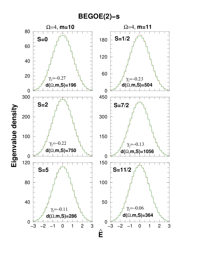
Figure 1: (Color online) Ensemble averaged eigenvalue density $\rho^{m,S}(\widehat{E})$ vs $\widehat{E}$ for BEGOE(2)-${\bf s}$ ensembles with $\Omega=4$, $m=10$ and $\Omega=4$, $m=11$. In the figure, histograms constructed with a bin size $0.2$ are BEGOE(2)-${\bf s}$ results and they are compared with Gaussian (dashed red) and Edgeworth (ED) corrected Gaussian (solid green) forms. The ensemble averaged values of the excess parameter $(\gamma_{2})$ are also shown in the figure. In the plots, the area under the curves is normalized to the dimensions $d(\Omega,m,S)$. See text for further details.

We have considered a 500 member BEGOE(2)-${\bf s}$ ensemble with $\Omega=4$ and $m=10$ and similarly a 100 member ensemble with $\Omega=4$ and $m=11$. Here and in all other numerical results presented in the paper, we use $\lambda_{0}=\lambda_{1}=\lambda$. In the construction of the ensemble averaged eigenvalue densities, the spectra of each member of the ensemble is first zero centered and scaled to unit width (therefore the densities are independent of the $\lambda$ parameter). The eigenvalues are then denoted by $\widehat{E}$. Given the fixed-($m,S$) energy centroids $E_{c}(m,S)$ and spectral widths $\sigma(m,S)$, $\widehat{E}=[E-E_{c}(m,S)]/\sigma(m,S)$. Then the histograms for the density are generated by combining the eigenvalues $\widehat{E}$ from all the members of the ensemble. Results are shown in Fig. 1 for a few selected $S$ values. The calculations have been carried out for all $S$ values (the results for other $S$ values are close to those given in the figure) and also for many other BEGOE(2)-${\bf s}$ examples. It is clearly seen that the eigenvalue densities are close to Gaussian (denoted by ${\cal G}$ below) with the ensemble averaged skewness ($\gamma_{1}$) and excess ($\gamma_{2}$) being very small; $|\gamma_{1}|\sim 0$, $|\gamma_{2}|\sim 0.1-0.27$. The agreements with Edgeworth (ED) corrected Gaussians are excellent. The ED form that includes $\gamma_{1}$ and $\gamma_{2}$ corrections is given by

$$\begin{array}[]{rcl}\eta_{ED}({\widehat{E}})&=&\eta_{{\cal G}}({\widehat{E}})\left\{1+\left[{\displaystyle\frac{\gamma_{1}}{6}}He_{3}\left({\widehat{E}}\right)\right]+\left[{\displaystyle\frac{\gamma_{2}}{24}}He_{4}\left({\widehat{E}}\right)+{\displaystyle\frac{\gamma_{1}^{2}}{72}}He_{6}\left({\widehat{E}}\right)\right]\right\}\;;\\ \eta_{{\cal G}}({\widehat{E}})&=&\displaystyle\frac{1}{\sqrt{2\pi}}\exp\left(-\displaystyle\frac{{\widehat{E}}^{2}}{2}\right)\;.\end{array}$$ (7)

Here, $He$ are Hermite polynomials: $He_{3}(x)=x^{3}-3x$, $He_{4}(x)=x^{4}-6x^{2}+3$ and $He_{6}(x)=x^{6}-15x^{4}+45x^{2}-15$.

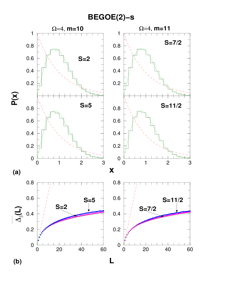
Figure 2: (Color online) (a) Ensemble averaged nearest neighbor spacing distribution (NNSD) and (b) Dyson-Mehta statistic $\overline{\Delta_{3}}(L)$ vs $L$ for $L\leq 60$. Results are for the same systems considered in Fig. 1; first column gives the results for ($\Omega=4$, $m=10$) and the second column for ($\Omega=4$, $m=11$) systems. The NNSD histograms from BEGOE(2)-${\bf s}$ are compared with Poisson (dashed red) and GOE (Wigner) forms (solid green) and similarly the $\overline{\Delta_{3}}(L)$ results. In the NNSD graphs, the bin-size is $0.2$ and $x$ is the nearest neighbor spacing in the units of local mean spacing. See text and Fig. 1 for further details.

For the analysis of level fluctuations (equivalent to studying the two-point function for the eigenvalues), each spectrum in the ensemble is unfolded using a sixth order polynomial correction to the Gaussian and then the smoothed density is $\overline{\eta(\widehat{E})}=\eta_{{\cal G}}(\widehat{E})\{1+\sum_{\zeta\geq 3}^{\zeta_{0}}(\zeta!)^{-1}S_{\zeta}He_{\zeta}(\widehat{E})\}$ with $\zeta_{0}=6$ Le-08 ; PDPK . The parameters $S_{\zeta}$ are determined by minimizing $\Delta^{2}=\sum_{i=1}^{d(\Omega,m,S)}[F(E_{i})-\overline{F(E)}]^{2}$. The distribution function $F(E)=\int_{-\infty}^{E}\eta(x)dx$ and similarly $\overline{F(E)}$ is defined. We require that the continuous function $\overline{F(E)}$ passes through the mid-points of the jumps in the discrete $F(E)$ and therefore, $F(E_{i})=(i-1/2)$. The ensemble averaged $\Delta_{RMS}$ is $\sim 3$ for $\zeta_{0}=3$, $\sim 1$ for $\zeta_{0}=4$ and $\sim 0.8$ for $\zeta_{0}=6$ with some variation with respect to $S$. As $\Delta_{RMS}\sim 0.88$ for GOE, this implies GOE fluctuations set in when we add 6th order corrections to the asymptotic Gaussian density. Using the unfolded energy levels of all the members of the BEGOE(2)-${\bf s}$ ensemble, the nearest neighbor spacing distribution (NNSD) that gives information about level repulsion and the Dyson-Mehta $\overline{\Delta_{3}}(L)$ statistic that gives information about spectral rigidity are studied. Results for the same systems used in Fig. 1 are shown in Fig. 2 for $S=2$ and $5$ (for other spins, the results are similar). In the calculations, middle 80% of the eigenvalues from each member are employed. It is clearly seen from the figures that the NNSD are close to GOE (Wigner) form and the widths of the NNSD are $\sim 0.288$ (GOE value is $\sim 0.272$). The $\overline{\Delta_{3}}(L)$ values show some departures from GOE for $L\mathrel{\mathchoice{\vbox{\offinterlineskip\halign{\hfil$\displaystyle#$\hfil\cr>\cr\sim\cr}}}{\vbox{\offinterlineskip\halign{\hfil$\textstyle#$\hfil\cr>\cr\sim\cr}}}{\vbox{\offinterlineskip\halign{ \hfil$\scriptstyle#$\hfil\cr>\cr\sim\cr}}}{\vbox{\offinterlineskip\halign{\hfil$\scriptscriptstyle# $\hfil\cr>\cr\sim\cr}}}}30$ for $S=S_{max}$ and this could be because the matrix dimensions are small for $S=S_{max}$ in our examples (also the systems considered are not strictly in the dense limit and numerical examples with much larger $m$ and $\Omega$ with $m>>\Omega$ are currently not feasible). It is useful to add that $S=S_{max}$ states are important for boson systems with random interactions as discussed in Sections IV-VI ahead. In conclusion, sixth order unfolding removes essentially all the secular behavior and then the fluctuations follow closely GOE. This is similar to the result known before for spinless boson systems Le-08 ; Ch-03 .

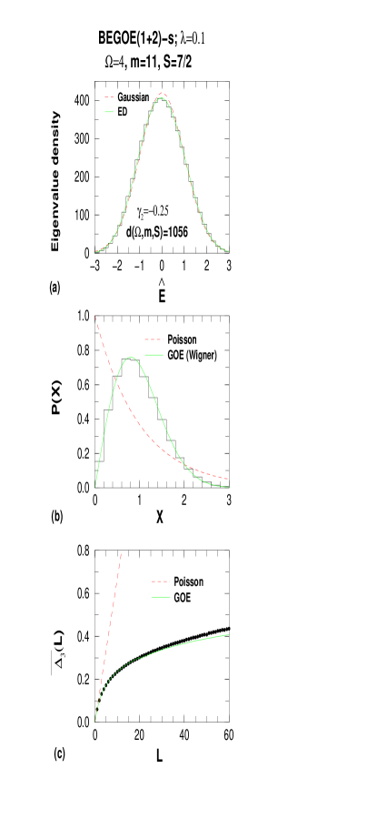
Figure 3: (Color online) (a) Ensemble averaged eigenvalue density $\rho^{m,S}(\widehat{E})$, (b) NNSD and (c) $\overline{\Delta_{3}}(L)$ vs. $L$ for a 100 member BEGOE(1+2)-${\bf s}$ ensemble for $\Omega=4$, $m=11$ and $S=7/2$ system with $\lambda_{0}=\lambda_{1}=\lambda=0.1$ in Eq. (1). For all other details, see text and Figs. 1 and 2.

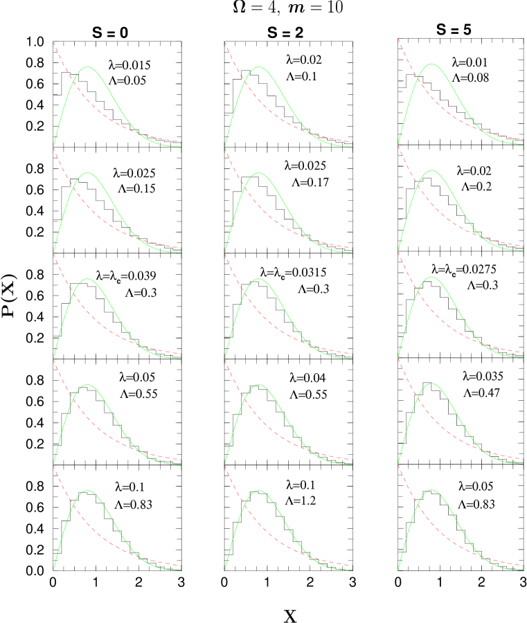
Figure 4: (Color online) NNSD for a 100 member BEGOE(1+2)-${\bf s}$ ensemble with $\Omega=4$, $m=10$ and spins $S=0$, $2$ and $5$. Calculated NNSD are compared to the Poisson (red dashed) and Wigner (GOE) (green solid) forms. Values of the interaction strength $\lambda$ and the transition parameter $\Lambda$ are given in the figure. The values of $\Lambda$ are deduced as discussed in Ma-10 . The chaos marker $\lambda_{c}$ corresponds to $\Lambda=0.3$ and its values, as shown in the figure, are $0.039,\;0.0315,\;0.0275$ for $S=0,\;2$ and 5 respectively. Bin-size for the histograms is $0.2$.

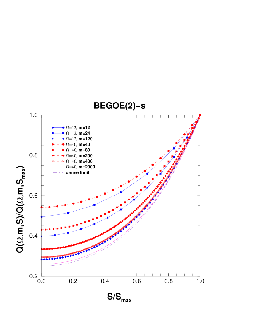
Figure 5: (Color online) BEGOE(2)-${\bf s}$ variance propagator Q($\Omega$,$m$,$S$)/Q($\Omega$, $m$,$S_{max}$) vs $S/S_{max}$ for various values of $\Omega$ and $m$. Formula for Q($\Omega$,$m$,$S$) follows from Eqs. (10), (13) and (14). Note that the results in the figure are for $\lambda_{0}=\lambda_{1}=\lambda$ in Eq. (6) and therefore independent of $\lambda$. Dense limit (dot-dashed) curve corresponds to the result due to Eq. (19) with $m=2000$.

Going beyond BEGOE(2)-${\bf s}$, calculations are also carried out for BEGOE(1+2)-${\bf s}$ systems using Eq. (1) with $\lambda_{0}=\lambda_{1}=\lambda$. We have verified the Gaussian behavior for the eigenvalue density for BEGOE(1+2)-${\bf s}$; an example is shown in Fig. 3a. This result is essentially independent of $\lambda$. In addition, we have also verified that BEGOE(1+2)-${\bf s}$ also generates level fluctuations close to GOE for $\lambda\mathrel{\mathchoice{\vbox{\offinterlineskip\halign{\hfil$\displaystyle#$\hfil\cr>\cr\sim\cr}}}{\vbox{\offinterlineskip\halign{\hfil$\textstyle#$\hfil\cr>\cr\sim\cr}}}{\vbox{\offinterlineskip\halign{ \hfil$\scriptstyle#$\hfil\cr>\cr\sim\cr}}}{\vbox{\offinterlineskip\halign{\hfil$\scriptscriptstyle# $\hfil\cr>\cr\sim\cr}}}}0.1$ for $\Omega=4$ and $m=10$, $11$ systems. Figure 3 shows an example with $\lambda=0.1$. Going beyond this, in Fig. 4, we show the NNSD results, for a 100 member BEGOE(1+2)-${\bf s}$ ensemble with $\Omega=4,\;m=10$ and total spins $S=0,\;2$ and $5$, for $\lambda$ varying from 0.01 to 0.1 to demonstrate that as $\lambda$ increases from zero, there is generically Poisson to GOE transition. A similar study has been reported in Ma-10 for fermion systems. As discussed there, for very small $\lambda$, the NNSD will be Poisson (as we use sp energies to be $\epsilon_{i}=i+1/i$, the $\lambda=0$ limit will not give strictly a Poisson). Moreover, as discussed in detail in Ma-10 , the variance of the NNSD can be written in terms of a parameter $\Lambda$ ($\Lambda$ is a parameter in a 2$\times$2 random matrix model that generates Poisson to GOE transition) with $\Lambda=0$ giving Poisson, $\Lambda\mathrel{\mathchoice{\vbox{\offinterlineskip\halign{\hfil$\displaystyle#$\hfil\cr>\cr\sim\cr}}}{\vbox{\offinterlineskip\halign{\hfil$\textstyle#$\hfil\cr>\cr\sim\cr}}}{\vbox{\offinterlineskip\halign{ \hfil$\scriptstyle#$\hfil\cr>\cr\sim\cr}}}{\vbox{\offinterlineskip\halign{\hfil$\scriptscriptstyle# $\hfil\cr>\cr\sim\cr}}}}1$ GOE and $\Lambda=0.3$ the transition point $\lambda_{c}$ that marks the onset of GOE fluctuations. We show in Fig. 4, for each $\lambda$, the deduced value of $\Lambda$ from the variance of the NNSD (Fig. 2 gives results for $\lambda\to\infty$ for $S=2$ and 5). As seen from the Fig. 4, $\lambda_{c}=0.039,\;0.0315,\;0.0275$ for $S=0$, $2$ and $5$ respectively. Thus $\lambda_{c}$ decreases with increasing spin $S$ and this is opposite to the situation for fermion systems. For a fixed $\Omega$ value, as discussed in Ma-10 , the $\lambda_{c}$ is inversely proportional to $K$, where $K$ is the number of many-particle states [defined by $h(1)$] that are directly coupled by the two-body interaction. For fermion systems, $K$ is proportional to the variance propagator but not for boson systems as discussed in Ch-03 . At present, for BEGOE(1+2)-${\bf s}$ we don’t have a formula for $K$. However, if we use the variance propagator $Q(\Omega,m,S)$ for the boson systems [see Eq. (14) and Fig. 5 ahead], then qualitatively we understand the decrease in $\lambda_{c}$ with increasing spin.

Finally, it is well known that the Gaussian form for the eigenvalue density is generic for embedded ensembles of spinless fermion Ko-01 and boson KP-80 ; Ch-03 systems. In addition, ensemble averaged fixed-($m,S$) eigenvalue densities for the fermion EGOE(1+2)-${\bf s}$ are shown to take Gaussian form in Ko-06a ; Ma-10 . Hence, from the results shown in Figs. 1 and 3a, it is plausible to conclude that the Gaussian form is generic for EE (both bosonic and fermionic) with good quantum numbers. With the eigenvalue density being close to Gaussian, it is useful to derive formulas for the energy centroids and ensemble averaged spectral variances. These in turn, as discussed ahead, will also allow us to study the lowest two moments of the two-point function. From now on, we will drop the ‘hat’over the operators $H$, $h(1)$ and $V(2)$.

IV Energy centroids, spectral variances and ensemble averaged spectral variances and covariances

IV.1 Propagation formulas for energy centroids and spectral variances

Given a general (1+2)-body Hamiltonian $H=h(1)+V(2)$, which is a typical member of BEGOE(1+2)-${\bf s}$, the energy centroids will be polynomials in the number operator and the $S^{2}$ operator. As $H$ is of maximum body rank 2, the polynomial form for the energy centroids is $\left\langle H\right\rangle^{m,S}=E_{c}(m,S)=a_{0}+a_{1}m+a_{2}m^{2}+a_{3}S(S+1)$. Solving for the $a$’s in terms of the centroids in one and two particle spaces, the propagation formula for the energy centroids is,

$$\begin{array}[]{rcl}\left\langle H\right\rangle^{m,S}=E_{c}(m,S)&=&\left[\left\langle h(1)\right\rangle^{1,\frac{1}{2}}\right]\;m+\lambda_{0}\,\left\langle\left\langle V^{s=0}(2)\right\rangle\right\rangle^{2,0}\;\displaystyle\frac{P^{0}(m,S)}{4\Omega(\Omega-1)}\\ &+&\lambda_{1}\,\left\langle\left\langle V^{s=1}(2)\right\rangle\right\rangle^{2,1}\;\displaystyle\frac{P^{1}(m,S)}{4\Omega(\Omega+1)}\;\;;\\ P^{0}(m,S)&=&\left[m(m+2)-4S(S+1)\right]\;\;,\\ P^{1}(m,S)&=&\left[3m(m-2)+4S(S+1)\right]\;\;,\\ \left\langle h(1)\right\rangle^{1,\frac{1}{2}}&=&\overline{\epsilon}=\Omega^{-1}\;\displaystyle\sum_{i=1}^{\Omega}\;\epsilon_{i}\;\;,\\ \left\langle\left\langle V^{s=0}(2)\right\rangle\right\rangle^{2,0}&=&\displaystyle\sum_{i<j}\;V^{s=0}_{ijij}\;,\;\;\;\left\langle\left\langle V^{s=1}(2)\right\rangle\right\rangle^{2,1}=\displaystyle\sum_{i\leq j}\;V^{s=1}_{ijij}\;.\end{array}$$ (8)

For the energy centroid of a two-body Hamiltonian [member of a BEGOE(2)-${\bf s}$], the $h(1)$ part in Eq. (8) will be absent.

Just as for the energy centroids, polynomial form for the spectral variances

$$\sigma_{H=h(1)+V(2)}^{2}(m,S)=\left\langle H^{2}\right\rangle^{m,S}-\left[E_{c}(m,S)\right]^{2}$$

is $\sum_{p=0}^{4}a_{p}m^{p}+\sum_{q=0}^{2}b_{q}m^{q}S(S+1)+c_{0}[S(S+1)]^{2}$. It is well known that the propagation formulas for fermion systems will give the formulas for the corresponding boson systems by applying $\Omega\rightarrow-\Omega$ transformation Ko-79 ; KP-80 ; Ko-81 ; Cv-82 ; Ko-05 . Applying this transformation to the propagation equation for the spectral variances for fermion systems with spin given by Eq. (8) of Ko-06a , we obtain the propagation equation for $\sigma_{H=h(1)+V(2)}^{2}(m,S)$ in terms of inputs that contain the single particle energies $\epsilon_{i}$ defining $h(1)$ and the two particle matrix elements $V_{ijkl}^{s}$. The final result is,

$$\begin{array}[]{l}\sigma_{H=h(1)+V(2)}^{2}(m,S)=\left\langle H^{2}\right\rangle^{m,S}-\left[E_{c}(m,S)\right]^{2}\\ \\ =\displaystyle\frac{(\Omega-2)mm^{\star}+2\Omega\;\left\langle S^{2}\right\rangle}{(\Omega-1)\Omega(\Omega+1)}\;\;\displaystyle\sum_{i}\;{\tilde{\epsilon}}_{i}^{2}\\ +\displaystyle\frac{m^{\star}P^{0}(m,S)}{2(\Omega-1)\Omega(\Omega+1)}\;\;\displaystyle\sum_{i}\;{\tilde{\epsilon}}_{i}\lambda_{i,i}(0)\\ +\displaystyle\frac{(\Omega-2)m^{\star}P^{1}(m,S)+8\Omega(m-1)\left\langle S^{2}\right\rangle}{2(\Omega-1)\Omega(\Omega+1)(\Omega+2)}\;\;\displaystyle\sum_{i}\;{\tilde{\epsilon}}_{i}\lambda_{i,i}(1)\\ +P^{\nu=1,s=0}(m,S)\;\;\displaystyle\sum_{i,j}\;\lambda_{i,j}^{2}(0)+P^{\nu=1,s=1}(m,S)\;\;\displaystyle\sum_{i,j}\;\lambda_{i,j}^{2}(1)\\ +\displaystyle\frac{P^{2}(m,S)P^{0}(m,S)}{4(\Omega-1)\Omega(\Omega+1)(\Omega+2)}\;\;\displaystyle\sum_{i,j}\;\lambda_{i,j}(0)\lambda_{i,j}(1)\\ +P^{\nu=2,s=0}(m,S)\,\left\langle\left(V^{\nu=2,s=0}\right)^{2}\right\rangle^{2,0}+P^{\nu=2,s=1}(m,S)\,\left\langle\left(V^{\nu=2,s=1}\right)^{2}\right\rangle^{2,1}\;;\end{array}$$ (9)

The propagators $P^{\nu,s}$’s, which are used later, are

$$\begin{array}[]{l}P^{\nu=1,s=0}(m,S)=\displaystyle\frac{\left[(m+2)m^{\star}/2-\left\langle S^{2}\right\rangle\right]P^{0}(m,S)}{8(\Omega-2)(\Omega-1)\Omega(\Omega+1)}\;,\\ P^{\nu=1,s=1}(m,S)=\displaystyle\frac{8\Omega(m-1)(\Omega+2m-4)\left\langle S^{2}\right\rangle+(\Omega-2)P^{2}(m,S)P^{1}(m,S)}{8(\Omega-1)\Omega(\Omega+1)(\Omega+2)^{2}}\;,\\ P^{\nu=2,s=0}(m,S)=\left[m^{\star}(m^{\star}-1)-\left\langle S^{2}\right\rangle\right]P^{0}(m,S)/[8\Omega(\Omega+1)]\;,\\ \\ P^{\nu=2,s=1}(m,S)=\left\{\left[\left\langle S^{2}\right\rangle\right]^{2}(3\Omega^{2}+7\Omega+6)/2+3m(m-2)m^{\star}(m^{\star}+1)\times\right.\\ \left.(\Omega-1)(\Omega-2)/8+\left[\left\langle S^{2}\right\rangle/2\right]\left[(5\Omega+3)(\Omega-2)mm^{\star}+\Omega(\Omega-1)(\Omega+1)(\Omega-6)\right]\right.\}/\\ \left[(\Omega-1)\Omega(\Omega+2)(\Omega+3)\right]\;;\\ P^{2}(m,S)=3(m-2)m^{\star}/2+\left\langle S^{2}\right\rangle\;,\;\;\;\;m^{\star}=\Omega+m/2\;,\;\;\;\;\left\langle S^{2}\right\rangle=S(S+1)\;.\end{array}$$ (10)

The inputs in Eq. (9) are given by,

$$\begin{array}[]{l}{\tilde{\epsilon}}_{i}=\epsilon_{i}-\overline{\epsilon}\;,\\ \lambda_{i,i}(s)=\displaystyle\sum_{j}\;V_{ijij}^{s}\;(1+\delta_{ij})\;-\;(\Omega)^{-1}\;\displaystyle\sum_{k,l}\;V^{s}_{klkl}\;(1+\delta_{kl})\;,\\ \lambda_{i,j}(s)=\displaystyle\sum_{k}\;\displaystyle\sqrt{(1+\delta_{ki})(1+\delta_{kj})}\,V^{s}_{kikj}\;\;\;\mbox{for}\;\;\;i\neq j\;,\\ V^{\nu=2,s}_{ijij}=V^{s}_{ijij}-\left[\left\langle V(2)\right\rangle^{2,s}+(\lambda_{i,i}(s)+\lambda_{j,j}(s))\left(\Omega-2(-1)^{s}\right)^{-1}\right]\;,\\ V^{\nu=2,s}_{kikj}=V^{s}_{kikj}-\left(\Omega-2(-1)^{s}\right)^{-1}\,\displaystyle\sqrt{(1+\delta_{ki})(1+\delta_{kj})}\,\lambda^{s}_{i,j}\;\;\;\mbox{for}\;\;\;i\neq j\;,\\ V^{\nu=2,s}_{ijkl}=V^{s}_{ijkl}\;\;\;\mbox{for all other cases}\;.\end{array}$$ (11)

Eqs. (8) and (9) can be applied to individual members of the BEGOE(1+2) ensemble. On the other hand, it is possible to use these to obtain ensemble averaged spectral variances and ensemble averaged covariances in energy centroids just as it was done before for fermion systems Ma-10 . Now we will consider these.

IV.2 Ensemble averaged spectral variances for BEGOE(2)-${\bf s}$

In this subsection, we restrict to $H=V(2)$, i.e. BEGOE(2)-${\bf s}$ and consider BEGOE(1+2)-${\bf s}$ at the end.

For the ensemble averaged spectral variances generated by $H$, only the fourth, fifth, seventh and eighth terms in Eq. (9) will contribute. Evaluating the ensemble averages of the inputs in these four terms, we obtain,

$$\begin{array}[]{l}\overline{\displaystyle\sum_{i,j}\;\lambda_{i,j}^{2}(0)}=\lambda_{0}^{2}(\Omega-1)(\Omega-2)(\Omega+2)\;,\\ \overline{\displaystyle\sum_{i,j}\;\lambda_{i,j}^{2}(1)}=\lambda_{1}^{2}(\Omega-1)(\Omega+2)^{2}\;,\\ \overline{\left\langle\left(H^{\nu=2,s=0}\right)^{2}\right\rangle^{2,0}}=\lambda_{0}^{2}\displaystyle\frac{(\Omega-3)(\Omega^{2}+\Omega+2)}{2(\Omega-1)}\;,\\ \overline{\left\langle\left(H^{\nu=2,s=1}\right)^{2}\right\rangle^{2,1}}=\lambda_{1}^{2}\displaystyle\frac{(\Omega-1)(\Omega+2)}{2}\;.\end{array}$$ (12)

Note that these inputs follow from the results for EGOE(2)-${\bf s}$ for fermions given in Ma-10 by interchanging $s=0$ with $s=1$. Now the final expression for the ensemble averaged variances is

$$\begin{array}[]{rcl}\overline{\sigma^{2}_{H}(m,S)}&=&\displaystyle\sum_{s=0,1}\lambda_{s}^{2}(\Omega-1)(\Omega-(-1)^{s}2)(\Omega+2)\;P^{\nu=1,s}(m,S)\\ &+&\lambda_{0}^{2}\displaystyle\frac{(\Omega-3)(\Omega^{2}+\Omega+2)}{2(\Omega-1)}\;P^{\nu=2,s=0}(m,S)\\ &+&\lambda_{1}^{2}\displaystyle\frac{(\Omega-1)(\Omega+2)}{2}\;P^{\nu=2,s=1}(m,S)\;.\end{array}$$ (13)

In most of the numerical calculations, we employ $\lambda_{0}=\lambda_{1}=\lambda$ and then $\overline{\sigma^{2}_{H}(m,S)}$ takes the form,

$$\overline{\sigma^{2}_{H}(m,S)}\stackrel{{\scriptstyle\lambda_{0}=\lambda_{1}=\lambda}}{{\longrightarrow}}\lambda^{2}Q(\Omega,m,S)\;.$$ (14)

Expression for the variance propagator $Q(\Omega,m,S)$ follows easily from Eqs. (8), (10) and (13). In Fig. 5, we show a plot of $Q(\Omega,m,S)/Q(\Omega,m,S_{max})$ vs $S/S_{max}$ for various $\Omega$ and $m$ values. It is clearly seen that the propagator value increases as spin increases and this is just opposite to the result for fermion systems Ma-10 . An important consequence of this is BEGOE(2)-${\bf s}$ gives ground states with $S=S_{max}$ [for fermion EGOE(2)-${\bf s}$, the ground states with random interactions have $S=0$]. This result follows from the Jacquod and Stone JS-01 criterion and according to this (from the assumption of Gaussian form for the eigenvalue densities), the gs energy $E_{gs}$ is given by $E_{gs}\propto-\displaystyle\sqrt{\overline{\sigma^{2}_{H}(m,S)}}$.

Before proceeding further, let us remark that for the BEGOE(1+2)-${\bf s}$ Hamiltonian $\{H\}=h(1)+\{V(2)\}$, assuming that $h(1)$ is fixed, we have $\overline{\sigma^{2}_{H}}=\sigma^{2}_{h(1)}+\overline{\sigma^{2}_{V(2)}}$. The first term $\sigma^{2}_{h(1)}$ is given by the first term of Eq. (9) and the second term is given by Eq. (13). In the situation $h(1)$ is represented by an ensemble independent of $\{V(2)\}$, we have to replace $\sigma^{2}_{h(1)}$ by $\overline{\sigma^{2}_{h(1)}}$ in $\overline{\sigma^{2}_{H}}$.

IV.3 Ensemble averaged covariances in energy centroids and spectral variances for BEGOE(2)-${\bf s}$

Normalized covariances in energy centroids and spectral variances are defined by

$$\begin{array}[]{rcl}\Sigma_{11}(m,S:m^{\prime},S^{\prime})&=&\displaystyle\frac{\overline{\left\langle H\right\rangle^{m,S}\left\langle H\right\rangle^{m^{\prime},S^{\prime}}}-\left\{\overline{\left\langle H\right\rangle^{m,S}}\right\}\;\;\left\{\overline{\left\langle H\right\rangle^{m^{\prime},S^{\prime}}}\right\}}{\displaystyle\sqrt{\left\{\overline{\left\langle H^{2}\right\rangle^{m,S}}\right\}\;\;\left\{\overline{\left\langle H^{2}\right\rangle^{m^{\prime},S^{\prime}}}\right\}}}\;,\\ \\ \Sigma_{22}(m,S:m^{\prime},S^{\prime})&=&\displaystyle\frac{\overline{\left\langle H^{2}\right\rangle^{m,S}\left\langle H^{2}\right\rangle^{m^{\prime},S^{\prime}}}-\left\{\overline{\left\langle H^{2}\right\rangle^{m,S}}\right\}\;\;\left\{\overline{\left\langle H^{2}\right\rangle^{m^{\prime},S^{\prime}}}\right\}}{\left\{\overline{\left\langle H^{2}\right\rangle^{m,S}}\right\}\;\;\left\{\overline{\left\langle H^{2}\right\rangle^{m^{\prime},S^{\prime}}}\right\}}\;.\end{array}$$ (15)

These define the lowest two moments of the two-point function,

$${\cal S}^{\Omega,m,S:\Omega,m^{\prime},S^{\prime}}(E,W)=\overline{\rho^{m,S}(E)\rho^{m^{\prime},S^{\prime}}(W)}-\left\{\overline{\rho^{m,S}(E)}\right\}\;\;\left\{\overline{\rho^{m^{\prime},S^{\prime}}(W)}\right\}\;.$$ (16)

For $(m,S)=(m^{\prime},S^{\prime})$ they will give information about fluctuations and in particular about level motion in the ensemble PDPK . For $(m,S)\neq(m^{\prime},S^{\prime})$, the covariances (cross correlations) are non-zero for BEGOE while they will be zero for independent GOE representation for the $m$ boson Hamiltonian matrices with different $m$ or $S$. Note that the $\Omega$ value has to be same for both $(m,S)$ and $(m^{\prime},S^{\prime})$ systems so that the Hamiltonian in two-particle spaces remains same. Now we will discuss analytical and numerical results for $\Sigma_{11}$ and numerical results for $\Sigma_{22}$ for large values of $(\Omega,m)$ and they are obtained using the results in Section IV.

Trivially, the ensemble average of the energy centroids $E_{c}(m,S)$ will be zero [note that $H$ is two-body for BEGOE(2)-${\bf s}$], i.e. $\overline{\left\langle H\right\rangle^{m,S}}=0$. However the covariances in the energy centroids of $H$ are non-zero and Eq. (8) gives,

$$\begin{array}[]{l}\overline{\left\langle H\right\rangle^{m,S}\left\langle H\right\rangle^{m^{\prime},S^{\prime}}}=\\ \displaystyle\frac{\lambda^{2}_{0}}{16\Omega(\Omega-1)}P^{0}(m,S)\,P^{0}(m^{\prime},S^{\prime})+\displaystyle\frac{\lambda^{2}_{1}}{16\Omega(\Omega+1)}P^{1}(m,S)\,P^{1}(m^{\prime},S^{\prime})\;.\end{array}$$ (17)

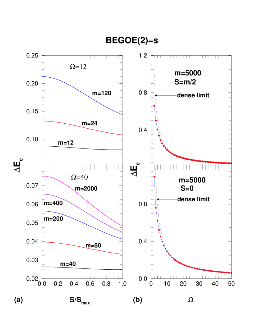
Figure 6: (Color online) (a) Self-correlations $\Sigma^{1/2}_{11}$ in energy centroids, giving width $\Delta E_{c}$ of the fluctuations in energy centroids scaled to the spectrum width, as a function of spin $S$ for different values of $m$ and $\Omega$. (b) Self correlations as a function of $\Omega$ for 5000 bosons with minimum spin $(S=0)$ and maximum spin $(S=2500)$. Dense limit (dot-dashed) curves for $S=0$ and $S=m/2$ in (b) correspond to the results given by Eq. (21). See text for details.

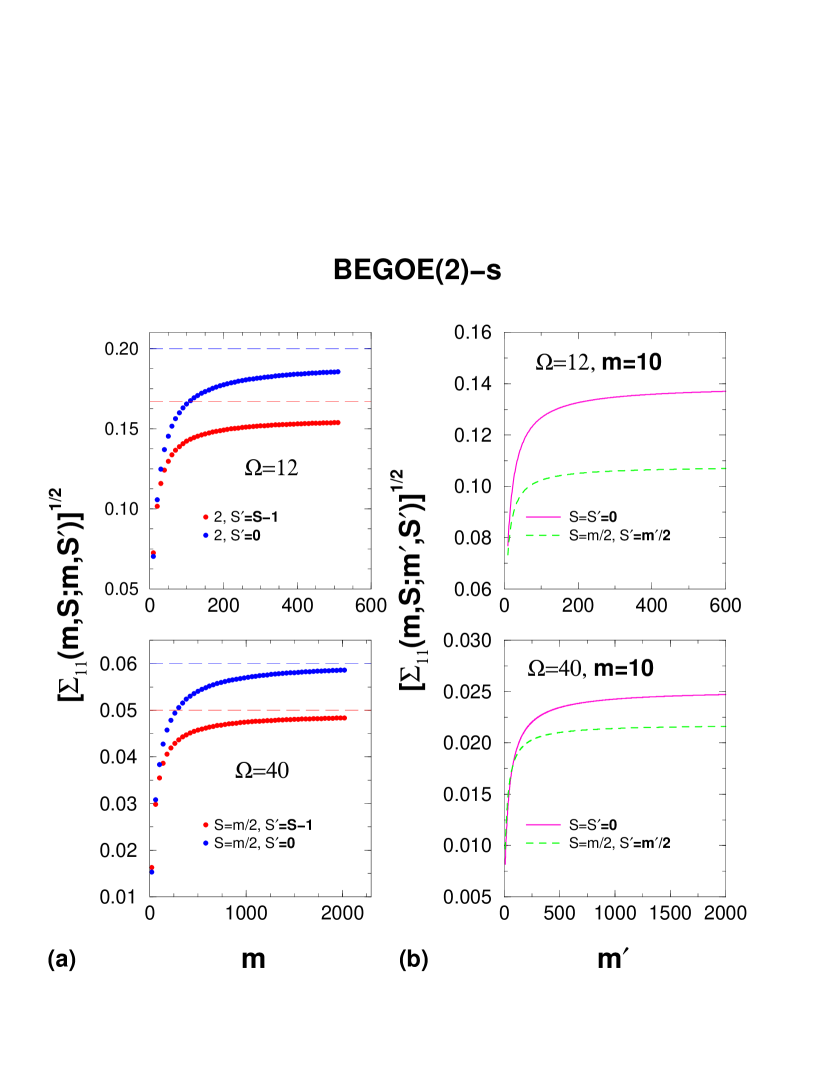
Figure 7: (Color online) Cross-correlations $\Sigma^{1/2}_{11}$ in energy centroids for various BEGOE(2)-${\bf s}$ systems. (a) $\Sigma^{1/2}_{11}$ vs $m$ with $m=m^{\prime}$ but different spins $(S\neq S^{\prime})$. (b) $\Sigma^{1/2}_{11}$ vs $m^{\prime}$ with $m=10$ and $S=S^{\prime}=0$ and $S=5,S^{\prime}=m^{\prime}/2$. The dashed lines in (a) are the dense limit results. See text for details.

Equations (13), (14) and (17) allow us to calculate $\Sigma_{11}$ for any $(\Omega,m,S)$. For $m=m^{\prime}$ and $S=S^{\prime}$, the $[\Sigma_{11}]^{1/2}$ gives the width $\Delta E_{c}$ of the fluctuations in the energy centroids. In the numerical calculations, we use $\lambda_{0}=\lambda_{1}=\lambda$ and therefore, $\Sigma_{11}$ and $\Sigma_{22}$ are independent of $\lambda$. Figure 6 gives some numerical results for $\Delta E_{c}$ and it is seen that : (i) for $m>>\Omega$, the ${\Delta}E_{c}$ is $\sim 20$% for $S=0$ and it goes down to $\sim 15$% for $S=S_{max}=m/2$ for $\Omega=12$; (ii) going from $\Omega=12$ to $40$, $\Delta E_{c}$ decreases to $\sim 2-7$%; (iii) for fixed $(m,\Omega)$, there is decrease in $\Delta E_{c}$ with increasing $S$ value; (iv) for fixed $(m,S)$ and very large $m$ value, there is a sharp decrease in $\Delta E_{c}$ with increasing $\Omega$ up to $\Omega\sim 20$ and then it slowly converges to zero. It is possible to understand these results and the results for cross correlations $[\Sigma_{11}(m,S:m^{\prime},S^{\prime})]^{1/2}$, with $(m,S)\neq(m^{\prime},S^{\prime})$ as shown in Fig. 7, using the asymptotic structure of $Q(\Omega,m,S)$.

Let us consider the dense limit defined by $m\rightarrow\infty$, $\Omega\rightarrow\infty$ and $m/\Omega\rightarrow\infty$. Firstly the $P^{{\nu},s}(m,S)$ in Eq. (10) take the simpler forms, with $S^{2}=S(S+1)$,

$$\begin{array}[]{l}P^{\nu=1,s=0}=\displaystyle\frac{\left(m^{2}-4S^{2}\right)^{2}}{32\Omega^{4}}\;,\;\;\;\;P^{\nu=1,s=1}=\displaystyle\frac{64m^{2}S^{2}\left(3m^{2}+4S^{2}\right)^{2}}{32\Omega^{4}}\;,\\ \\ P^{\nu=2,s=0}=\displaystyle\frac{\left(m^{2}-4S^{2}\right)^{2}}{32\Omega^{2}}\;,\;\;\;\;P^{\nu=2,s=1}=\displaystyle\frac{3m^{4}+40m^{2}S^{2}+48(S^{2})^{2}}{32\Omega^{2}}\;.\end{array}$$ (18)

Using these in Eq. (13), with $\lambda_{0}=\lambda_{1}=\lambda$, we have

$$\begin{array}[]{l}\overline{\sigma_{H}^{2}(m,S)}=\lambda^{2}\displaystyle\frac{\left(m^{2}+4S^{2}\right)^{2}}{16}\;;\\ \Rightarrow\overline{\sigma_{H}^{2}(m,S)}/\overline{\sigma_{H}^{2}(m,S_{max})}=\left[\displaystyle\frac{m/(m+2)+S^{2}/S_{max}^{2}}{m/(m+2)+1}\right]^{2}\;.\end{array}$$ (19)

The dense limit result given by Eq. (19) with $m=2000$ is compared with the exact results in Fig. 5. Firstly, it should be noted that for the applicability of Eq. (19), $\Omega$ should be sufficiently large and $m>>\Omega$. Also, the result is independent of $\Omega$. Comparing with the $\Omega=12$ and $\Omega=40$ results, it is seen that the dense limit result is very close to the $\Omega=40$ results for $m\mathrel{\mathchoice{\vbox{\offinterlineskip\halign{\hfil$\displaystyle#$\hfil\cr>\cr\sim\cr}}}{\vbox{\offinterlineskip\halign{\hfil$\textstyle#$\hfil\cr>\cr\sim\cr}}}{\vbox{\offinterlineskip\halign{ \hfil$\scriptstyle#$\hfil\cr>\cr\sim\cr}}}{\vbox{\offinterlineskip\halign{\hfil$\scriptscriptstyle# $\hfil\cr>\cr\sim\cr}}}}200$. Thus for sufficiently large value of $\Omega$ and $m\mathrel{\mathchoice{\vbox{\offinterlineskip\halign{\hfil$\displaystyle#$\hfil\cr>\cr\sim\cr}}}{\vbox{\offinterlineskip\halign{\hfil$\textstyle#$\hfil\cr>\cr\sim\cr}}}{\vbox{\offinterlineskip\halign{ \hfil$\scriptstyle#$\hfil\cr>\cr\sim\cr}}}{\vbox{\offinterlineskip\halign{\hfil$\scriptscriptstyle# $\hfil\cr>\cr\sim\cr}}}}5\Omega$, the dense limit result describes quite well the exact results.

Simplifying $\overline{\left\langle H\right\rangle^{m,S}\left\langle H\right\rangle^{m^{\prime},S^{\prime}}}$ gives in the dilute limit,

$$\begin{array}[]{l}\overline{\left\langle H\right\rangle^{m,S}\left\langle H\right\rangle^{m^{\prime},S^{\prime}}}=\\ \displaystyle\frac{\lambda^{2}}{16\Omega^{2}}\left[\left(m^{2}-4S^{2}\right)\left\{(m^{\prime})^{2}-4(S^{\prime})^{2}\right\}+\left(3m^{2}+4S^{2}\right)\left\{3(m^{\prime})^{2}+4(S^{\prime})^{2}\right\}\right]\;.\end{array}$$ (20)

Then $[\Sigma_{11}]^{1/2}$, with $m=m^{\prime}$ and $S=S^{\prime}$ (for $\lambda_{0}=\lambda_{1}$) giving $\Delta E_{c}$, is

$$[\Sigma_{11}]^{1/2}=\Delta E_{c}=\displaystyle\frac{\displaystyle\sqrt{2(5m^{4}+8m^{2}S^{2}+16(S^{2})^{2})}}{\Omega\left(m^{2}+4S^{2}\right)}\;.$$ (21)

Eq. (21) gives $[\Sigma_{11}]^{1/2}$ to be $\sqrt{10}/\Omega$ and $2/\Omega$ for $S=0$ and $S=S_{max}$ and these dense limit results are well verified by the results in Fig. 6b. Similarly, Eqs. (19) and (20) will give $[\Sigma_{11}]^{1/2}$ to be $\sqrt{6}/\Omega$ for $(m=m^{\prime}:S=S_{max},S^{\prime}=0)$ and $2/\Omega$ for $(m=m^{\prime}:S=S_{max},S^{\prime}=S_{max}-1)$. The upper and lower dashed lines in Fig. 7a for $\Omega=12$ (similarly for $\Omega=40$) correspond to these two dense limit results respectively. It is seen that the dense limit results are close to exact results for $\Omega=40$ but there are deviations for $\Omega=12$. Also, for $\Omega=40$, the agreements are good only for $m\mathrel{\mathchoice{\vbox{\offinterlineskip\halign{\hfil$\displaystyle#$\hfil\cr>\cr\sim\cr}}}{\vbox{\offinterlineskip\halign{\hfil$\textstyle#$\hfil\cr>\cr\sim\cr}}}{\vbox{\offinterlineskip\halign{ \hfil$\scriptstyle#$\hfil\cr>\cr\sim\cr}}}{\vbox{\offinterlineskip\halign{\hfil$\scriptscriptstyle# $\hfil\cr>\cr\sim\cr}}}}80$ and these are similar to the results discussed earlier with reference to Fig. 5.

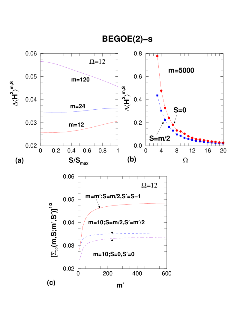
Figure 8: (Color online) Correlations in spectral variances $\Sigma^{1/2}_{22}$ for various BEGOE(2)-${\bf s}$ systems. (a) Self-correlations, giving width $\Delta\left\langle H^{2}\right\rangle^{m,S}$ of the spectral variances, as a function of spin $S$ for $m=12$, $24$ and $120$ with $\Omega=12$. (b) Self-correlations as a function of $\Omega$ for 5000 bosons with $S=0$ and $2500$. (c) Three examples for cross-correlation in spectral variances with same or different particle numbers and same or different spins. All the results are obtained using 500 member ensembles. See text for details.

Unlike for the covariances in energy centroids, we do not have at present complete analytical formulation for the covariances in spectral variances. However, for a given member of BEGOE(2)-${\bf s}$, generating numerically (on a computer) the ensembles $\{V^{s=0}(2)\}$ and $\{V^{s=1}(2)\}$ and applying Eqs. (8) and (9) to each member of the ensemble will give $\overline{\left\langle H^{2}\right\rangle^{m.S}}=\overline{\sigma^{2}(m,S)}+\overline{\left[E_{c}(m,S)\right]^{2}}$. This procedure has been used with 500 members and results for $\Sigma_{22}$ are obtained for various $({\Omega},m,S)$ values. For some examples, results are shown in Fig. 8 for both self correlations giving the width $\Delta\left\langle H^{2}\right\rangle^{m,S}$ of variances and cross correlations $[\Sigma_{22}]^{1/2}$ with $(m,S)\neq(m^{\prime},S^{\prime})$. It is seen that $[\Sigma_{22}]^{1/2}$ are always much smaller than $[\Sigma_{11}]^{1/2}$ just as for EGOE(2) for spinless fermion systems Ko-06a . It is seen from Fig. 8a that for $\Omega=12$, width of the fluctuations in the variances $\left\langle H^{2}\right\rangle^{m,S}$ are $\sim 3-5$%. Similarly for large $m$, with $\Omega$ very small, the widths are quite large but they decrease fast with increasing $\Omega$ as seen from Fig. 8b. Finally, for $\Omega=12$, the cross correlations are $\sim 4$%.

Besides the moments $\Sigma_{11}$ and $\Sigma_{22}$, it is possible to numerically construct the two-point function ${\cal S}^{\Omega,m,S:\Omega,m^{\prime},S^{\prime}}(E,W)$ using the eigenvalues from the BEGOE(2)-${\bf s}$ Hamiltonian matrices in small examples. We have carried out the calculations for ${\cal S}^{4,10,0:4,10,1}(E,W)$ using a 500 member BEGOE(2)-${\bf s}$ ensemble. It is seen that the structure of ${\cal S}(E,W)$ is similar to the nuclear shell model examples reported in PW-06 and EGOE(1+2)-${\bf s}$ example in Ma-10c . The maximum value of ${\cal S}^{4,10,0:4,10,1}(E,W)$ is found to be $\sim 7$% of $\overline{\rho^{10,0}(E)}\,\times\,\overline{\rho^{10,1}(W)}$. Let us add that it is important to identify measures involving $\Sigma_{11}$ and $\Sigma_{22}$ and also ${\cal S}^{\Omega,m,S:\Omega,m^{\prime},S^{\prime}}(E,W)$, $(m,S)\neq(m^{\prime},S^{\prime})$ that can be tested using some experiments so that evidence for BEGOE(2) operation in real quantum systems can be established.

V Preponderance of $S_{max}=m/2$ ground states and natural spin order : role of exchange interaction

V.1 Introduction to regular structures with random interactions

Johnson et al Jo-98 discovered in 1998 that the nuclear shell model with random interactions generates, with high probability, $0^{+}$ ground states in even-even nuclei (also generates odd-even staggering in binding energies, the seniority pairing gap etc.) and similarly, Bijker and Frank BF-00 found that the interacting boson model ($sd$IBM) of atomic nuclei [in this model, one considers identical bosons carrying angular momentum $\ell=0$ (called $s$ bosons) and $\ell=2$ (called $d$ bosons)] with random interactions generates vibrational and rotational structures with high probability. Starting with these, there are now many studies on regular structures in many-body systems generated by random interactions. See for example Zh-04 ; Zel-04 ; We-09 for reviews on the subject. More recently, the effect of random interactions in the $pn$-$sd$IBM with $F$-spin quantum number has been studied by Yoshida et al Yo-09 . Here, proton and neutron bosons are treated as the two components of a spin $\frac{1}{2}$ boson and this spin is called $F$-spin. Yoshida et al found that random interactions conserving $F$-spin generate predominance of maximum $F$-spin ($F_{max}$) ground states. It should be noted that the low-lying states generated by $pn$-$sd$IBM correspond to those of $sd$IBM and all $sd$IBM states will have $F=F_{max}$. Thus random interactions preserve the property that the low-lying states generated by $pn$-$sd$IBM are those of $sd$IBM. Similarly, using shell model with isospin conserving interactions (here protons and neutrons correspond to the two projections of isospin ${\bf t}=\frac{1}{2}$), Kirson and Mizrahi Ki-07 showed that random interactions generate natural isospin ordering. Denoting the lowest energy state (les) for a given many nucleon isospin $T$ by $E_{les}(T)$, the natural isospin ordering corresponds to $E_{les}(T_{min})\leq E_{les}(T_{min}+1)\leq\ldots$; for even-even N=Z nuclei, $T_{min}=0$. Therefore, one can ask if BEGOE(1+2)-${\bf s}$ generates a spin ordering.

As an application of BEGOE(1+2)-${\bf s}$, we present here results for the probability of gs spin to be $S=S_{max}$ and also for natural spin ordering (NSO). Here NSO corresponds to $E_{les}(S_{max})\leq E_{les}(S_{max}-1)\ldots$. In this analysis, we add the Majorana force or the space exchange operator to the Hamiltonian in Eq. (1). Note that $S$ in BEGOE(1+2)-${\bf s}$ is similar to $F$-spin in the $pn$-$sd$IBM. First we will derive the exchange interaction and then present some numerical results.

V.2 $U(\Omega)$ algebra and space exchange operator

In terms of boson creation ($b^{\dagger}$) and annihilation ($b$) operators, the sp states for $(\Omega)^{m}$ systems are $\left.\left|i,m_{\bf s}\pm\frac{1}{2}\right.\right\rangle=b^{\dagger}_{i,\frac{1}{2},m_{\bf s}}\left|0\right\rangle$ with $i=1,2,\ldots,\Omega$. It can be easily identified that the 4$\Omega^{2}$ number of one-body operators $A_{ij;\mu}^{r}$,

$$A_{ij;\mu}^{r}=\left(b_{i}^{\dagger}\tilde{b_{j}}\right)_{\mu}^{r}\;;\;\;\;\;r=0,\;1\,,$$ (22)

generate $U(2\Omega)$ algebra. In Eq. (22), $\tilde{b}_{i,\frac{1}{2},m_{\bf s}}=(-1)^{\frac{1}{2}+m_{\bf s}}b_{i,\frac{1}{2},-m_{\bf s}}$. The $U(2\Omega)$ irreducible representations (irreps) are denoted trivially by the particle number $m$ as they must be symmetric irreps $\{m\}$. The $\Omega^{2}$ number of operators $A_{ij}^{0}$ generate $U(\Omega)$ algebra and similarly there is a $U(2)$ algebra generated by the number operator $\hat{n}$ and the spin generators $S^{1}_{\mu}$,

$$\begin{array}[]{l}\hat{n}=\displaystyle\sqrt{2}\displaystyle\sum_{i}A_{ii}^{0}\;;\;\;\;\;S^{1}_{\mu}=\displaystyle\frac{1}{\sqrt{2}}\displaystyle\sum_{i}A_{ii;\mu}^{1}\;.\end{array}$$ (23)

Then we have the group-subgroup algebra $U(2\Omega)\supset U(\Omega)\otimes SU(2)$ with $SU(2)$ generated by $S^{1}_{\mu}$. As the $U(2)$ irreps are two-rowed, the $U(\Omega)$ irreps have to be two-rowed and they are labeled by $\{m_{1},m_{2}\}$ with $m=m_{1}+m_{2}$ and $S=(m_{1}-m_{2})/2$; $m_{1}\geq m_{2}\geq 0$. Thus with respect to $U(\Omega)\otimes SU(2)$ algebra, many boson states are labeled by $\left|\{m_{1},m_{2}\},\xi\right\rangle$ or equivalently by $\left|(m,S),\xi\right\rangle$, where $\xi$ are extra labels required for a complete specification of the states. The quadratic Casimir operator of the $U(\Omega)$ algebra is,

$$C_{2}[U(\Omega)]=2\displaystyle\sum_{i,j}A_{ij}^{0}\cdot A_{ji}^{0}$$ (24)

and its eigenvalues are $\left\langle C_{2}[U(\Omega)]\right\rangle^{\{m_{1},m_{2}\}}=m_{1}(m_{1}+\Omega-1)+m_{2}(m_{2}+\Omega-3)$ or equivalently,

$$\left\langle C_{2}[U(\Omega)]\right\rangle^{(m,S)}=\displaystyle\frac{m}{2}(2\Omega+m-4)+2S(S+1)\;.$$ (25)

Note that the Casimir invariant of $SU(2)$ is $\hat{S}^{2}$ with eigenvalues $S(S+1)$. Now we will show that the space exchange or the Majorana operator ${\widehat{M}}$ is simply related to $C_{2}\left[U(\Omega)\right]$.

Majorana operator ${\widehat{M}}$ acting on a two-particle state exchanges the spatial coordinates of the particles (index $i$) and leaves the spin quantum numbers ($m_{\bf s}$) unchanged. The operator form of ${\widehat{M}}$ is

$${\widehat{M}}=\displaystyle\frac{\kappa}{2}\displaystyle\sum_{i,j,m_{\bf s},m_{\bf s}^{\prime}}\left(b^{\dagger}_{j,m_{\bf s}}b^{\dagger}_{i,m_{\bf s}^{\prime}}\right)\left(b^{\dagger}_{i,m_{\bf s}}b^{\dagger}_{j,m_{\bf s}^{\prime}}\right)^{\dagger}\;.$$ (26)

Equation (26) gives, with $\kappa$ a constant,

$${\widehat{M}}=\displaystyle\frac{\kappa}{2}\left\{C_{2}\left[U(\Omega)\right]-\Omega\hat{n}\right\}\;.$$ (27)

Then, combining Eqs. (25) and (27), we have

$${\widehat{M}}=\kappa\left\{\hat{n}\left(\displaystyle\frac{\hat{n}}{4}-1\right)+\hat{S}^{2}\right\}\;.$$ (28)

As seen from Eq. (28), exchange interaction with $\kappa>0$ generates gs with $S=S_{min}=0$($\frac{1}{2}$) for even(odd) $m$ (this is opposite to the result for fermion systems where the exchange interaction generates gs with $S=S_{max}=m/2$ Ma-10c ; JS-01 ). Now we will study the interplay between random interactions and the Majorana force in generating gs spin structure in boson systems. Note that for states with boson number fixed, ${\widehat{M}}\propto\hat{S}^{2}$ as seen from Eq. (28) and therefore, from now on, we refer to $\hat{S}^{2}$ as the exchange interaction.

V.3 Numerical results for $S_{max}=m/2$ ground states and natural spin order

In order to understand the gs structure in BEGOE(1+2)-${\bf s}$, we have studied $P(S=S_{max})$, the probability for the gs to be with spin $S_{max}=m/2$, by adding the exchange term $\lambda_{S}\,S^{2}$ with $\lambda_{S}>0$ to the Hamiltonian in Eq. (1), i.e. using

$$\{H\}_{\mbox{BEGOE(1+2)-{\bf s}}:\mbox{Exch}}=h(1)+\lambda\,\left[\,\{V^{s=0}(2)\}+\{V^{s=1}(2)\}\,\right]\,+\lambda_{S}\,S^{2}\;.$$ (29)

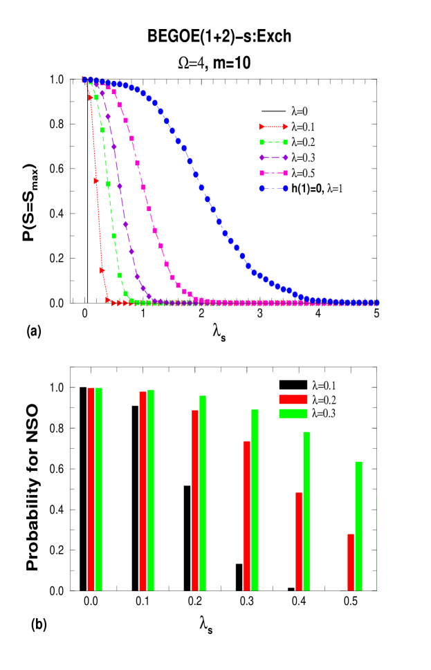
Figure 9: (Color online) (a) Probability for ground states to have spin $S=S_{max}$ as a function of the exchange interaction strength $\lambda_{S}\geq 0$. (b) Probability for natural spin order (NSO) as a function of $\lambda_{S}$. Results are shown for a 500 member BEGOE(1+2)-${\bf s}:\mbox{Exch}$ ensemble generated by Eq. (29) for a system with $\Omega=4$ and $m=10$. Values of the interaction strength $\lambda$ are shown in the figure.

Note that the operator $S^{2}$ is simple in the $(m,S)$ basis. Fig. 9a gives probability $P(S=S_{max})$ for the ground states to have spin $S=S_{max}$ as a function of exchange interaction strength $\lambda_{S}$ for $\lambda_{0}=\lambda_{1}=\lambda=0$, $0.1$, $0.2$, $0.3$ and $0.5$ and also for $h(1)=0$ with $\lambda=1$. Similarly, Fig. 9b shows the results for NSO. Calculations are carried out for ($\Omega=4$, $m=10$) system using a 500 member ensemble and the mean-field Hamiltonian $h(1)$ is as defined in Section II.

V.3.1 Preponderance of $S_{max}=m/2$ ground states

Let us begin with pure random two-body interactions. Then $h(1)=0$ in Eq. (29). Now in the absence of the exchange interaction ($\lambda_{S}=0$), as seen from Fig. 9a, ground states will have $S=S_{max}$, i.e. the probability $P(S=S_{max})=1$. The variance propagator (see Fig. 5) derived earlier gives a simple explanation for this by applying the Jacquod and Stone prescription as discussed in Sec. IV B. Thus pure random interactions generate preponderance of $S=S_{max}$ ground states. On the other hand, as discussed in Section V B, the exchange interaction acts in opposite direction by generating $S=S_{min}$ ground states. Therefore, by adding the exchange interaction to the $\{V(2)\}$ ensemble, $P(S=S_{max})$ starts decreasing as the strength $\lambda_{S}$ ($\lambda_{S}>0$) starts increasing. For the example considered in Fig. 9a, for $\lambda_{S}>4$, we have $P(S=S_{max})\sim 0$. The complete variation with $\lambda_{S}$ is shown in Fig. 9a marked $h(1)=0$ and $\lambda=1$.

Similarly, on the other end, for $\lambda=0$ in Eq. (29), we have $H=h(1)$ in the absence of the exchange interaction. In this situation, as all the bosons can occupy the lowest sp state, gs spin $S=S_{max}$. Therefore, $P(S=S_{max})=1$. When the exchange interaction is turned on, $P(S=S_{max})$ remains unity until $\lambda_{S}$ equals the spacing between the lowest two sp states divided by $m$. As in our example, the sp energies are $\epsilon_{i}=i+1/i$, we have $P(S=S_{max})=1$ for $\lambda_{S}<0.05$. Then $P(S=S_{max})$ drops to zero for $\lambda_{S}\geq 0.05$. This variation with $\lambda_{S}$ is shown in Fig. 9a marked $\lambda=0$. Figure 9a also shows the variation of $P(S=S_{max})$ with $\lambda_{S}$ for several values of $\lambda$ between $0.1$ and $0.5$. It is seen that there is a critical value ($\lambda_{S}^{c}$) of $\lambda_{S}$ after which $P(S=S_{max})=0$ and its value increases with $\lambda$. Also, the variation of $P(S=S_{max})$ with $\lambda_{S}$ becomes slower as $\lambda$ increases.

In summary, results in Fig. 9a clearly show that with random interactions there is preponderance of $S=S_{max}=m/2$ ground states. This is unlike for fermions where there is preponderance of $S=S_{min}=0(\frac{1}{2})$ ground states for $m$ even(odd). With the addition of the exchange interaction, $P(S=S_{max})$ decreases and finally goes to zero for $\lambda_{S}\geq\lambda_{S}^{c}$ and the value of $\lambda_{S}^{c}$ increases with $\lambda$. We have also carried out calculations for ($\Omega=4$, $m=11$) system using a 100 member ensemble and the results are close to those given in Fig. 9a. All these explain the results given in Yo-09 where random interactions are employed within $pn$-$sd$IBM.

V.3.2 Natural spin ordering

For the system considered in Fig. 9a, for each member of the ensemble, eigenvalue of the lowest state for each spin $S$ is calculated and using these, we have obtained total number of members $N_{\lambda}$ having NSO as a function of $\lambda_{S}$ for $\lambda=0.1,0.2$ and $0.3$ using the Hamiltonian given in Eq. (29). As stated in Section V A, the NSO here corresponds to (as $S=S_{max}$ is the spin of the gs of the system) $E_{les}(S_{max})<E_{les}(S_{max}-1)<E_{les}(S_{max}-2)<\ldots$. The probability for NSO is $N_{\lambda}/500$ and the results are shown in Fig. 9b. In the absence of the exchange interaction, as seen from Fig. 9b, NSO is found in all the members independent of $\lambda$. Thus random interactions strongly favor NSO. The presence of exchange interaction reduces the probability for NSO. Comparing Figs. 9a and 9b, it is clearly seen that with increasing exchange interaction strength, probability for gs state spin to be $S=S_{max}$ is preserved for much larger values of $\lambda_{S}$ (with a fixed $\lambda$) compared to the NSO. Therefore for preserving both $S=S_{max}$ gs and the NSO with high probability, the $\lambda_{S}$ value has to be small. We have also verified this for the ($\Omega=4$, $m=11$) system. Finally, it is plausible to argue that the results in Fig. 9 obtained using BEGOE(1+2)-${\bf s}$ are generic for boson systems with spin. Now we will turn to pairing in BEGOE(2)-${\bf s}$.

VI Pairing in BEGOE(2)-${\bf s}$

Pairing correlations are known to be important not only for fermion systems but also for boson systems Pe-10 . An important issue that is raised in the recent years is: to what extent random interactions carry features of pairing. See Ma-10 ; Zh-04 ; Zel-04 ; Ho-07 for some results for fermion systems. In order to address this question for boson systems, first we will identify the pairing algebra in $(\Omega,m,S)$ spaces of BEGOE(2)-${\bf s}$. Then we will consider expectation values of the pairing Hamiltonian in the eigenstates generated by BEGOE(2)-${\bf s}$ as they carry signatures of pairing.

VI.1 $U(2\Omega)\supset[U(\Omega)\supset SO(\Omega)]\otimes SU_{S}(2)$ Pairing symmetry

In constructing BEGOE(2)-${\bf s}$, it is assumed that spin is a good symmetry and thus the $m$-particle states carry spin ($S$) quantum number. Now, following the $SO(5)$ pairing algebra for fermions Fl-64 , it is possible to consider pairs that are vectors in spin space. The pair creation operators $P_{i:\mu}$ for the level $i$ and the generalized pair creation operators (over the $\Omega$ levels) $P_{\mu}$, with $\mu=-1,0,1$, in spin coupled representation, are

$$P_{\mu}=\displaystyle\frac{1}{\sqrt{2}}\displaystyle\sum_{i}\left(b^{\dagger}_{i}b^{\dagger}_{i}\right)^{1}_{\mu}=\displaystyle\sum_{i}P_{i:\mu}\;,\;\;\;\left(P_{\mu}\right)^{\dagger}=\displaystyle\frac{1}{\sqrt{2}}\displaystyle\sum_{i}(-1)^{1-\mu}\left(\tilde{b_{i}}\tilde{b_{i}}\right)^{1}_{-\mu}\;.$$ (30)

Therefore in the space defining BEGOE(2)-$s$, the pairing Hamiltonian $H_{p}$ and its two-particle matrix elements are,

$$H_{p}=\displaystyle\sum_{\mu}P_{\mu}\left(P_{\mu}\right)^{\dagger}\;,\;\;\;\left\langle(k\ell)s\mid H_{p}\mid(ij)s\right\rangle=\delta_{s,1}\,\delta_{i,j}\,\delta_{k,\ell}\;.$$ (31)

With this, we will proceed to identify and analyze the pairing algebra. It is easy to verify that the $\Omega(\Omega-1)/2$ number of operators $C_{ij}=A_{ij}^{0}-A_{ji}^{0}$, $i>j$ generate a $SO(\Omega)$ subalgebra of the $U(\Omega)$ algebra. Therefore we have $U(2\Omega)\supset[U(\Omega)\supset SO(\Omega)]\otimes SU(2)$. We will show that the irreps of $SO(\Omega)$ algebra are uniquely labeled by the seniority quantum number $v$ and a reduced spin $\tilde{s}$ similar to the reduced isospin introduced in the context of nuclear shell model Fl-52 and they in turn define the eigenvalues of $H_{p}$. The quadratic Casimir operator of the $SO(\Omega)$ algebra is,

$$C_{2}[SO(\Omega)]=2\displaystyle\sum_{i>j}C_{ij}\cdot C_{ji}\;.$$ (32)

Carrying out angular momentum algebra Ed-77 it can be shown that,

$$C_{2}[SO(\Omega)]=C_{2}[U(\Omega)]-2\,H_{p}-\hat{n}\;.$$ (33)

The quadratic Casimir operator of the $U(\Omega)$ algebra is given in Eq. (24). Before discussing the eigenvalues of the pairing Hamiltonian $H_{p}$, let us first consider the irreps of $SO(\Omega)$.

Given the two-rowed $U(\Omega)$ irreps $\{m_{1},m_{2}\}$; $m_{1}+m_{2}=m$, $m_{1}-m_{2}=2S$, it should be clear that the $SO(\Omega)$ irreps should be of $[v_{1},v_{2}]$ type and for later simplicity we use $v_{1}+v_{2}=v$ and $v_{1}-v_{2}=2\tilde{s}$. The quantum number $v$ is called seniority and $\tilde{s}$ is called reduced spin. The $SO(\Omega)$ irreps for a given $\{m_{1},m_{2}\}$ can be obtained as follows. First expand the $U(\Omega)$ irrep $\{m_{1},m_{2}\}$ in terms of totally symmetric irreps,

$$\{m_{1},m_{2}\}=\{m_{1}\}\times\{m_{2}\}-\{m_{1}+1\}\times\{m_{2}-1\}\;.$$ (34)

Note that the irrep multiplication in Eq. (34) is a Kronecker multiplication Ko-06b ; Wy-70 . For a totally symmetric $U(\Omega)$ irrep $\{m^{\prime}\}$, the $SO(\Omega)$ irreps are given by the well-known result

$$\{m^{\prime}\}\to[v]=[m^{\prime}]\oplus[m^{\prime}-2]\oplus\ldots\oplus[0]\mbox{ or }[1]\;.$$ (35)

Finally, reduction of the Kronecker product of two symmetric $SO(\Omega)$ irreps $[v_{1}]$ and $[v_{2}]$, $\Omega>3$ into $SO(\Omega)$ irreps $[v_{1},v_{2}]$ is given by (for $v_{1}\geq v_{2}$) Ko-06b ; Wy-70 ,

$$[v_{1}]\times[v_{2}]=\displaystyle\sum_{k=0}^{v_{2}}\displaystyle\sum_{r=0}^{v_{2}-k}[v_{1}-v_{2}+k+2r,k]\oplus\;.$$ (36)

Combining Eqs. (34), (35) and (36) gives the $\{m_{1},m_{2}\}\to[v_{1},v_{2}]$ reductions. It is easy to implement this procedure on a computer.

Given the space defined by $\left|\{m_{1},m_{2}\},[v_{1},v_{2}],\alpha\right\rangle$, with $\alpha$ denoting extra labels needed for a complete specification of the state, the eigenvalues of $C_{2}[SO(\Omega)]$ are Ko-06b

$$\left\langle C_{2}[SO(\Omega)]\right\rangle^{\{m_{1},m_{2}\},[v_{1},v_{2}]}=v_{1}(v_{1}+\Omega-2)+v_{2}(v_{2}+\Omega-4)\;.$$ (37)

Now changing $\{m_{1},m_{2}\}$ to $(m,S)$ and $[v_{1},v_{2}]$ to $(v,\tilde{s})$ and using Eqs. (33) and (25) will give the formula for the eigenvalues of the pairing Hamiltonian $H_{p}$. The final result is,

$$E_{p}(m,S,v,\tilde{s})=\left\langle H_{p}\right\rangle^{m,S,v,\tilde{s}}=\displaystyle\frac{1}{4}(m-v)(2\Omega-6+m+v)+[S(S+1)-\tilde{s}(\tilde{s}+1)]\;.$$ (38)

This is same as the result that follows from Eq. (18) of Fl-64 for fermions by using $\Omega\to-\Omega$ symmetry. From now on, we denote the $U(\Omega)$ irreps by $(m,S)$ and $SO(\Omega)$ irreps by $(v,\tilde{s})$. In Table LABEL:red, for $(\Omega,m)=(4,10),(5,8)$ and $(6,6)$ systems, given are the $(m,S)\to(v,\tilde{s})$ reductions, the pairing eigenvalues given by Eq. (38) in the spaces defined by these irreps and also the dimensions of the $U(\Omega)$ and $SO(\Omega)$ irreps. The dimensions $d(\Omega,m,S)$ of the $U(\Omega)$ irreps $(m,S)$ are given by Eq. (2). Similarly, the dimension ${\mbox{\boldmath$d$}}(v_{1},v_{2})\Leftrightarrow{\mbox{\boldmath$d$}}(v,\tilde{s})$ of the $SO(\Omega)$ irreps $[v_{1},v_{2}]$ follow from Eqs. (35) and (36) and they will give

$$\begin{array}[]{l}{\mbox{\boldmath$d$}}(v_{1},v_{2})={\mbox{\boldmath$d$}}(v_{1}){\mbox{\boldmath$d$}}(v_{2})-\displaystyle\sum_{k=0}^{v_{2}-1}\displaystyle\sum_{r=0}^{v_{2}-k}{\mbox{\boldmath$d$}}(v_{1}-v_{2}+k+2r,k)\;;\\ \\ {\mbox{\boldmath$d$}}(v)=\displaystyle\binom{\Omega+v-1}{v}-\displaystyle\binom{\Omega+v-3}{v-2}\;.\end{array}$$ (39)

Note that in general the $SO(\Omega)$ irreps $(v,\tilde{s})$ can appear more than once in the reduction of $U(\Omega)$ irreps $(m,S)$. For example, $(2,1)$ irrep of $SO(\Omega)$ appears twice in the reduction of the $U(\Omega)$ irrep $(10,1)$.

It is useful to remark that just as the fermionic $SO(5)$ pairing algebra for nucleons in $j$ orbits Pa-65 ; He-65 ; Fl-64 , there will be a $SO(4,1)$ complementary pairing algebra corresponding to the $SO(\Omega)$ subalgebra. The ten operators $P^{1}_{\mu}$, $(P^{1}_{\mu})^{\dagger}$, $S^{1}_{\mu}$ and $\hat{n}$ form the $SO(4,1)$ algebra. It is possible to exploit this algebra to derive properties of the eigenstates defined by the pairing Hamiltonian but this will be discussed elsewhere.

VI.2 Pairing expectation values

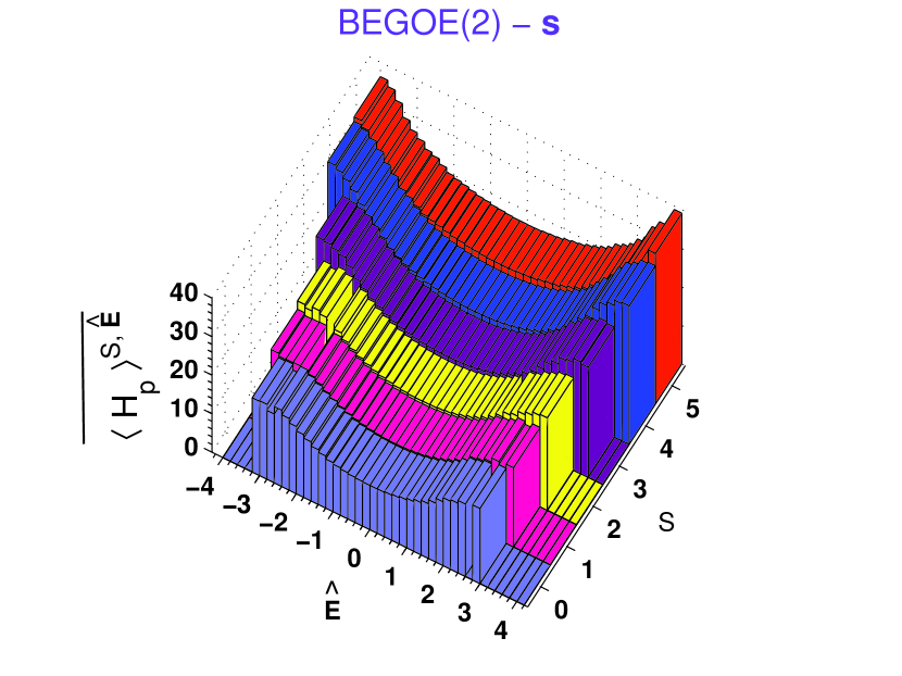
Figure 10: (Color online) Ensemble averaged pairing expectation values $\overline{\left\langle H_{p}\right\rangle^{S,\widehat{{\mbox{\boldmath$E$}}}}}$ vs $\widehat{{\mbox{\boldmath$E$}}}$ and $S$, shown as a 3D histogram, for a 500 member BEGOE(2)-${\bf s}$ ensemble with $\Omega=4$ and $m=10$. The bin-size is 0.2 for $\widehat{{\mbox{\boldmath$E$}}}$. Note that the $\widehat{{\mbox{\boldmath$E$}}}$ label in this figure is different from the $\widehat{E}$ used in Figs. 1 and 3a.

Pairing expectation values are defined by $\left\langle H_{p}\right\rangle^{S,E}=\left\langle m,S,E\mid H_{p}\mid m,S,E\right\rangle$ for eigenstates with energy $E$ and spin $S$ generated by a Hamiltonian $H$ for a system of $m$ bosons in $\Omega$ number of sp orbitals (for simplicity, we have dropped $\Omega$ and $m$ labels in $\left\langle H_{p}\right\rangle^{S,E}$). In our analysis, $H$ is a member of BEGOE(2)-${\bf s}$. As we will be comparing the results for all spins at a given energy $E$, for each member of the ensemble the eigenvalues for all spins are zero centered and normalized using the $m$-particle energy centroid $E_{c}(m)=\left\langle H\right\rangle^{m}$ and spectrum width $\sigma(m)=[\left\langle H^{2}\right\rangle^{m}-\{E_{c}(m)\}^{2}]^{1/2}$. Then the eigenvalues $E$ for all $S$ are changed to $\widehat{{\mbox{\boldmath$E$}}}=[E-E_{c}(m)]/\sigma(m)$. Using the method described in Section II, the $H_{p}$ matrix is constructed in good $M_{S}$ basis and transformed into the eigenbasis of a given $S$ for each member of the BEGOE(2)-${\bf s}$ ensemble. Then the ensemble average of the diagonal elements of the $H_{p}$ matrix will give the ensemble averaged pairing expectation values $\overline{\left\langle H_{p}\right\rangle^{S,E}}\Leftrightarrow\overline{\left\langle H_{p}\right\rangle^{S,\widehat{{\mbox{\boldmath$E$}}}}}$. Using this procedure for a 500 member BEGOE(2)-${\bf s}$ ensemble with $\Omega=4$, $m=10$ and $S=0-5$, results for $\overline{\left\langle H_{p}\right\rangle^{S,\widehat{{\mbox{\boldmath$E$}}}}}$ as a function of energy $\widehat{{\mbox{\boldmath$E$}}}$ (with $\widehat{{\mbox{\boldmath$E$}}}$ as described above) and spin $S$ are obtained and they are shown as a 3D histogram in Fig. 10. From Table LABEL:red, it is seen that the maximum value of the eigenvalues $E_{p}(m,S,v,\tilde{s})$ increases with spin $S$ for a fixed-$(\Omega,m)$. The values are $28$, $32$, $34$, $42$, $48$ and $60$ for $S=0-5$ respectively for $\Omega=4$ and $m=10$. Numerical results in Fig. 10 also show that for states near the lowest $\widehat{{\mbox{\boldmath$E$}}}$ value, $\overline{\left\langle H_{p}\right\rangle^{S,\widehat{{\mbox{\boldmath$E$}}}}}$ increases with spin $S$. Thus random interactions preserve this property of the pairing Hamiltonian in addition to generating $S=S_{max}$ ground states as discussed in Section V.3. It is useful to remark that random interactions will not generate $S=S_{max}$ ground states with $(v,\tilde{s})=(m,m/2)$ as required for example in the $pn$-$sd$IBM. This needs explicit inclusion of pairing and exchange terms in the Hamiltonians defined by Eqs. (1) and (6).

For a given spin $S$, the pairing expectation values as a function of $E$ are expected, for two-body ensembles, to be given by a ratio of expectation value density (EVD) Gaussian (the first two moments given by $\left\langle H_{p}H\right\rangle^{m,S}$ and $\left\langle H_{p}H^{2}\right\rangle^{m,S}$) and the eigenvalue density Gaussian with normalization given by $\left\langle H_{p}\right\rangle^{m,S}$ and this itself will be a Gaussian Ma-09 . Let us denote the EVD centroid by $E_{c}(m,S:H_{p})$ and width by $\sigma(m,S:H_{p})$. Then the ratio of Gaussians will give

$$\begin{array}[]{l}\overline{\left\langle H_{p}\right\rangle^{S,\widehat{E}}}=\displaystyle\frac{\left\langle H_{p}\right\rangle^{m,S}}{\widehat{\sigma}(m,S)}\exp{\displaystyle\frac{\widehat{\epsilon}^{2}(m,S)}{2\left[1-\widehat{\sigma}^{2}(m,S)\right]}}\;\exp\left\{\displaystyle\frac{(\widehat{\sigma}^{2}(m,S)-1)}{2\widehat{\sigma}^{2}(m,S)}\left[\widehat{E}-\displaystyle\frac{\widehat{\epsilon}(m,S)}{1-\widehat{\sigma}^{2}(m,S)}\right]^{2}\right\}\;.\end{array}$$ (40)

Here, $\widehat{\epsilon}(m,S)=\{E_{c}(m,S:H_{p})-E_{c}(m,S)\}/\sigma(m,S)$, $\widehat{\sigma}(m,S)=\sigma(m,S:H_{p})/\sigma(m,S)$ and $\widehat{E}=[\sigma(m)/\sigma(m,S)]\{\widehat{{\mbox{\boldmath$E$}}}-{\cal E}\}$; ${\cal E}=[E_{c}(m,S)-E_{c}(m)]/\sigma(m)$. The Gaussian form given by Eq. (40) is clearly seen in Fig. 10 and this also gives a quantitative description of the results. Note that in our example, $\widehat{\epsilon}(10,S)=0.001$, $0.001$, $0.001$, $0.002$, $0.002$, $0.003$ and $\widehat{\sigma}(10,S)=1.045$, $1.047$, $1.053$, $1.062$, $1.073$, $1.082$ respectively for $S=0-5$.

VII Conclusions

In the present work, we have introduced the BEGOE(1+2)-${\bf s}$ ensemble and a method for constructing BEGOE(1+2)-${\bf s}$ for numerical calculations has been described. Numerical examples are used to show that, like the spinless BEGOE(1+2), the spin BEGOE(1+2)-${\bf s}$ ensemble also generates Gaussian density of states in the dense limit. Similarly, BEGOE(2)-${\bf s}$ exhibits GOE level fluctuations. On the other hand, BEGOE(1+2)-${\bf s}$ exhibits Poisson to GOE transition as the interaction strength $\lambda$ is increased and the transition marker $\lambda_{c}$ is found to decrease with increasing spin. Moreover, ensemble averaged covariances in energy centroids and spectral variances for BEGOE(2)-${\bf s}$ between spectra with different particle numbers and spins are studied using the propagation formulas derived for the energy centroids and spectral variances. For $\Omega=12$ systems, the cross correlations in energy centroids are $\sim 15$% and they reduce to $\sim 4$% for spectral variances. We have also derived the exact formula for the ensemble averaged fixed-$(m,S)$ spectral variances and demonstrated that the variance propagator gives a simple explanation for the preponderance of spin $S=S_{max}$ ground states generated by random interactions as in $pn$-$sd$IBM. It is also shown, by including exchange interaction $\hat{S}^{2}$ in BEGOE(1+2)-${\bf s}$, that random interactions preserving spin symmetry strongly favor NSO (just as with isospin in nuclear shell model). In addition, we have identified the pairing $SO(\Omega)$ symmetry and showed using numerical examples that random interactions exhibit pairing correlations in the gs region and also they generate a Gaussian form for the variation of the pairing expectation values with respect to energy.

Results in this paper represent a beginning in systematic studies of BEGOE(1+2)-${\bf s}$ ensemble. To go beyond the present work requires: (i) dealing with systems with much larger $\Omega$ and $m$ values and then the matrix dimensions will be $10^{5}-10^{6}$ and higher; (ii) further group theoretical analysis for deriving higher moments of the two-point function and this requires new results for Wigner and Racah coefficients for general $U(\Omega)$ algebras (see for example Ma-10b ); and (iii) identifying and analyzing measures that can be used in experimental data analysis, say for example data from ultracold gases. With progress in (i) and (ii), it is possible to investigate more systematically BEGOE(1+2)-${\bf s}$ as a function of the strength parameter $\lambda$ by analyzing the delocalization and other related measures (see for example Ma-10 ; Sa-10 ; Sa-10a ). With these it is possible to address (iii) but this is for future.

Further extensions of BEGOE(1+2)-${\bf s}$ including ${\bf s}=1$, $2$, $\ldots$ degrees of freedom for bosons, as emphasized in the Introduction, are relevant for spinor BEC studies Pe-10 ; Yi-07 . These extended BEGOE’s will be explored in future. Finally, it is useful to mention that the numerical code developed for constructing BEGOE(1+2)-${\bf s}$ ensemble in fixed-$(m,S)$ spaces can be used in analyzing ensembles generated by Hamiltonians preserving only $M_{S}$. Here it is important to point out that, besides the $SO(\Omega)$ pairing discussed in Section VI, there is another pairing algebra that corresponds to $U(2\Omega)\supset SO(2\Omega)\supset[SO(\Omega)\otimes SO(2)]$ as pointed out in Ko-06b . The pairing Hamiltonian corresponding to this group-subgroup chain preserves only $M_{S}$ but not $S$ and hence, relevant for BEGOE(1+2) with fixed $M_{S}$.

APPENDIX A

Let us consider a system of $m$ spinless bosons occupying $N$ sp states $\left|\left.\nu_{i}\right\rangle\right.$, $i=1,2,\ldots,N$ and the Hamiltonian is say two-body. Then the Hamiltonian operator is

$$\widehat{H}=\displaystyle\sum_{\nu_{i}\leq\nu_{j},\;\nu_{k}\leq\nu_{l}}\displaystyle\frac{\left\langle\nu_{k}\;\nu_{l}\mid H\mid\nu_{i}\;\nu_{j}\right\rangle}{\displaystyle\sqrt{(1+\delta_{ij})(1+\delta_{kl})}}\;b^{\dagger}_{\nu_{k}}\,b^{\dagger}_{\nu_{l}}\,b_{\nu_{i}}\,b_{\nu_{j}}\;.$$ (A1)

with the symmetries for the symmetrized two-body matrix elements $\left\langle\nu_{k}\;\nu_{l}\mid H\mid\nu_{i}\;\nu_{j}\right\rangle$ being,

$$\begin{array}[]{c}\left\langle\nu_{k}\;\nu_{l}\mid H\mid\nu_{j}\;\nu_{i}\right\rangle=\left\langle\nu_{k}\;\nu_{l}\mid H\mid\nu_{i}\;\nu_{j}\right\rangle\;,\\ \left\langle\nu_{k}\;\nu_{l}\mid H\mid\nu_{i}\;\nu_{j}\right\rangle=\left\langle\nu_{i}\;\nu_{j}\mid H\mid\nu_{k}\;\nu_{l}\right\rangle\;.\\ \end{array}$$ (A2)

The Hamiltonian matrix $H(m)$ in $m$-particle spaces contains three different types of non-zero matrix elements and explicit formulas for these are PDPK ,

$$\begin{array}[]{l}\left\langle\displaystyle\prod_{r=i,j,\ldots}\left(\nu_{r}\right)^{n_{r}}\mid H\mid\displaystyle\prod_{r=i,j,\ldots}\left(\nu_{r}\right)^{n_{r}}\right\rangle=\displaystyle\sum_{i\geq j}\;\displaystyle\frac{n_{i}\left(n_{j}-\delta_{ij}\right)}{\left(1+\delta_{ij}\right)}\;\left\langle\nu_{i}\nu_{j}\mid H\mid\nu_{i}\nu_{j}\right\rangle\;,\\ \\ \left\langle\left(\nu_{i}\right)^{n_{i}-1}\left(\nu_{j}\right)^{n_{j}+1}\displaystyle\prod_{r^{\prime}=k,l,\ldots}\left(\nu_{r^{\prime}}\right)^{n_{r^{\prime}}}\mid H\mid\displaystyle\prod_{r=i,j,\ldots}\left(\nu_{r}\right)^{n_{r}}\right\rangle=\\ \\ \displaystyle\sum_{k^{\prime}}\;\left[\displaystyle\frac{n_{i}\left(n_{j}+1\right)\left(n_{k^{\prime}}-\delta_{k^{\prime}i}\right)^{2}}{\left(1+\delta_{k^{\prime}i}\right)\left(1+\delta_{k^{\prime}j}\right)}\right]^{1/2}\;\left\langle\nu_{k^{\prime}}\nu_{j}\mid H\mid\nu_{k^{\prime}}\nu_{i}\right\rangle\;,\\ \\ \left\langle\left(\nu_{i}\right)^{n_{i}+1}\left(\nu_{j}\right)^{n_{j}+1}\left(\nu_{k}\right)^{n_{k}-1}\left(\nu_{l}\right)^{n_{l}-1}\displaystyle\prod_{r^{\prime}=m,n,\ldots}\left(\nu_{r^{\prime}}\right)^{n_{r^{\prime}}}\mid H\mid\displaystyle\prod_{r=i,j,\ldots}\left(\nu_{r}\right)^{n_{r}}\right\rangle=\\ \\ \left[\displaystyle\frac{n_{k}\left(n_{l}-\delta_{kl}\right)\left(n_{i}+1\right)\left(n_{j}+1+\delta_{ij}\right)}{\left(1+\delta_{ij}\right)\left(1+\delta_{kl}\right)}\right]^{1/2}\;\left\langle\nu_{i}\nu_{j}\mid H\mid\nu_{k}\nu_{l}\right\rangle\;.\end{array}$$ (A3)

In the second equation in Eq. (A3), $i\neq j$ and in the third equation, four combinations are possible: (i) $k=l$, $i=j$, $k\neq i$; (ii) $k=l$, $i\neq j$, $k\neq i$, $k\neq j$; (iii) $k\neq l$, $i=j$, $i\neq k$, $i\neq l$; and (iv) $i\neq j\neq k\neq l$. BEGOE(2) for spinless boson systems is defined by Eqs. (A2) and (A3) with the $H$ matrix in two-particle spaces being GOE. Note that the $H(m)$ matrix dimension is $\binom{N+m-1}{m}$ and the number of independent matrix elements is $d_{2}(d_{2}+1)/2$ where $d_{2}=N(N+1)/2$. It is useful to mention that the formulas for the energy centroids and spectral variances in $m$-boson spaces follow from Eqs. (8), (9), (10) and (11) with $S=m/2$, putting the $s=0$ matrix elements to zero and replacing $\Omega$ by $N$.

Table 1: Classification of states in the $U(2\Omega)\supset$ $[U(\Omega)\supset SO(\Omega)]\otimes SU_{S}(2)$ limit for $(\Omega,m)=(4,10),(5,8)$ and $(6,6)$. Given are $U(\Omega)$ labels $(m,S)$ and $SO(\Omega)$ labels $(v,\tilde{s})$ with the corresponding dimensions $d(\Omega,m,S)$ and ${\mbox{\boldmath$d$}}(v,\tilde{s})$ respectively and also the pairing eigenvalues $E_{p}(m,S,v,\tilde{s})$. Note that $\sum_{v,\tilde{s}}r{\mbox{\boldmath$d$}}(v,\tilde{s})=d(\Omega,m,S)$; here $r$ denotes multiplicity of the $SO(\Omega)$ irreps and in the table, they are shown only for the cases when $r>1$.

$\Omega$	$m$	$(m,S)_{d(\Omega,m,S)}$	$(v,\tilde{s})^{r}_{{\mbox{\boldmath$d$}}(v,\tilde{s})}$	$E_{p}(m,S,v,\tilde{s})$	$\Omega$	$m$	$(m,S)_{d(\Omega,m,S)}$	$(v,\tilde{s})^{r}_{{\mbox{\boldmath$d$}}(v,\tilde{s})}$	$E_{p}(m,S,v,\tilde{s})$
$4$	$10$	$(10,0)_{196}$	$(2,0)_{6}$	$28$	$5$	$8$	$(8,0)_{490}$	$(0,0)_{1}$	$24$
			$(4,1)_{30}$	$22$				$(2,1)_{14}$	$19$
			$(6,2)_{70}$	$12$				$(4,2)_{55}$	$10$
			$(6,0)_{14}$	$18$				$(4,0)_{35}$	$16$
			$(8,1)_{54}$	$8$				$(6,1)_{220}$	$7$
			$(10,0)_{22}$	$0$				$(8,0)_{165}$	$0$
		$(10,1)_{540}$	$(2,1)^{2}_{9}$	$28$			$(8,1)_{1260}$	$(2,1)_{14}$	$21$
			$(4,2)^{2}_{25}$	$20$				$(4,2)_{55}$	$12$
			$(6,3)_{49}$	$8$				$(4,1)^{2}_{81}$	$16$
			$(4,1)_{30}$	$24$				$(6,2)_{260}$	$5$
			$(6,2)_{70}$	$14$				$(6,1)_{220}$	$9$
			$(6,1)^{2}_{42}$	$18$				$(8,1)_{455}$	$0$
			$(8,2)_{90}$	$6$				$(2,0)_{10}$	$23$
			$(8,1)_{54}$	$10$				$(6,0)_{84}$	$11$
			$(10,1)_{66}$	$0$			$(8,2)_{1500}$	$(4,2)^{2}_{55}$	$16$
			$(0,0)_{1}$	$32$				$(6,3)_{140}$	$3$
			$(4,0)_{10}$	$26$				$(6,2)_{260}$	$9$
			$(8,0)_{18}$	$12$				$(8,2)_{625}$	$0$
		$(10,2)_{750}$	$(4,2)^{2}_{25}$	$24$				$(2,1)^{2}_{14}$	$25$
			$(6,3)_{49}$	$12$				$(4,1)_{81}$	$20$
			$(6,2)^{2}_{70}$	$18$				$(6,1)_{220}$	$13$
			$(8,3)_{126}$	$4$				$(0,0)_{1}$	$30$
			$(8,2)_{90}$	$10$				$(4,0)_{35}$	$22$
			$(10,2)_{110}$	$0$			$(8,3)_{1155}$	$(6,3)_{140}$	$9$
			$(2,1)_{9}$	$32$				$(8,3)_{595}$	$0$
			$(4,1)^{2}_{30}$	$28$				$(4,2)_{55}$	$22$
			$(6,1)_{42}$	$22$				$(6,2)_{260}$	$15$
			$(8,1)_{54}$	$14$				$(2,1)_{14}$	$31$
			$(2,0)_{6}$	$34$				$(4,1)_{81}$	$26$
			$(6,0)_{14}$	$24$				$(2,0)_{10}$	$33$
		$(10,3)_{770}$	$(6,3)^{2}_{49}$	$18$			$(8,4)_{495}$	$(8,4)_{285}$	$0$
			$(8,4)_{81}$	$2$				$(6,3)_{140}$	$17$
			$(8,3)_{126}$	$10$				$(4,2)_{55}$	$30$
			$(10,3)_{154}$	$0$				$(2,1)_{14}$	$39$
			$(4,2)^{2}_{25}$	$30$				$(0,0)_{1}$	$44$
			$(6,2)_{70}$	$24$	$6$	$6$	$(6,0)_{490}$	$(2,0)_{15}$	$14$
			$(8,2)_{90}$	$16$				$(4,1)_{175}$	$6$
			$(2,1)^{2}_{9}$	$38$				$(6,0)_{300}$	$0$
			$(4,1)_{30}$	$34$			$(6,1)_{1134}$	$(2,1)^{2}_{20}$	$14$
			$(6,1)_{42}$	$28$				$(4,2)_{105}$	$4$
			$(0,0)_{1}$	$42$				$(4,1)_{175}$	$8$
			$(4,0)_{10}$	$36$				$(6,1)_{729}$	$0$
		$(10,4)_{594}$	$(8,4)_{81}$	$10$				$(0,0)_{1}$	$20$
			$(10,4)_{198}$	$0$				$(4,0)_{84}$	$10$
			$(6,3)_{49}$	$26$			$(6,2)_{1050}$	$(4,2)_{105}$	$8$
			$(8,3)_{126}$	$18$				$(6,2)_{735}$	$0$
			$(4,2)_{25}$	$38$				$(2,1)_{20}$	$18$
			$(6,2)_{70}$	$32$				$(4,1)_{175}$	$12$
			$(2,1)_{9}$	$46$				$(2,0)_{15}$	$20$
			$(4,1)_{30}$	$42$			$(6,3)_{462}$	$(6,3)_{336}$	$0$
			$(2,0)_{6}$	$48$				$(4,2)_{105}$	$14$
		$(10,5)_{286}$	$(10,5)_{121}$	$0$				$(2,1)_{20}$	$24$
			$(8,4)_{81}$	$20$				$(0,0)_{1}$	$30$
			$(6,3)_{49}$	$36$
			$(4,2)_{25}$	$48$
			$(2,1)_{9}$	$56$
			$(0,0)_{1}$	$60$

References

- (1) F. Haake, Quantum Signatures of Chaos, (Springer, New York, 2010).
- (2) J.B. French and S.S.M. Wong, Phys. Lett. B33, 449 (1970).
- (3) O. Bohigas and J. Flores, Phys. Lett. B34, 261 (1971).
- (4) K.K. Mon and J.B. French, Ann. Phys. (N.Y.) 95, 90 (1975).
- (5) V.K.B. Kota, Phys. Rep. 347, 223 (2001).
- (6) Manan Vyas, V.K.B. Kota, and N.D. Chavda, Phys. Rev. E 81, 036212 (2010).
- (7) J.M.G. Gómez, K. Kar, V.K.B. Kota, R.A. Molina, A. Relaño, and J. Retamosa, Phys. Rep. (2010), in press.
- (8) L. Benet, T. Rupp, and H.A. Weidenmüller, Ann. Phys. 292, 67 (2001).
- (9) V.K.B. Kota, J. Math. Phys. 46, 033514 (2005).
- (10) V.K.B. Kota, J. Math. Phys. 48, 053304 (2007).
- (11) Manan Vyas and V.K.B. Kota, Ann. Phys. (N.Y.) 325, 2451 (2010).
- (12) T.A. Brody, J. Flores, J.B. French, P.A. Mello, A. Pandey, and S.S.M. Wong, Rev. Mod. Phys. 53, 385 (1981).
- (13) R.J. Leclair, R.U. Haq, V.K.B. Kota, and N.D. Chavda, Phys. Lett. A372, 4373 (2008).
- (14) J.B. French, V.K.B. Kota, A. Pandey, and S. Tomsovic, Ann. Phys. (N.Y.) 181, 235 (1988).
- (15) T. Papenbrock and H.A. Weidenmüller, Rev. Mod. Phys. 79, 997 (2007).
- (16) V.K.B. Kota, Int. J. Mod. Phys. E 15, 1869 (2006).
- (17) V.K.B. Kota, N.D. Chavda, and R. Sahu, Phys. Lett. A359, 381 (2006).
- (18) Manan Vyas, V.K.B. Kota, and N.D. Chavda, Phys. Lett. A373, 1434 (2009).
- (19) Y. Alhassid, Rev. Mod. Phys. 72, 895 (2000).
- (20) T. Papenbrock, L. Kaplan, and G.F. Bertsch, Phys. Rev. B 65, 235120 (2002).
- (21) Ph. Jacquod and A.D. Stone, Phys. Rev. B 64, 214416 (2001).
- (22) Manan Vyas, arXiv:1004.2761.
- (23) W.G. Brown, L.F. Santos, D.J. Starling, and L. Viola, Phys. Rev. E 77, 021106 (2008).
- (24) M. Rigol, Phys. Rev. Lett. 103, 100403 (2009).
- (25) L.F. Santos and M. Rigol, Phys. Rev. E 81, 036206 (2010).
- (26) L.F. Santos and M. Rigol, arxiv:1006.0729.
- (27) M. Olshanii and V. Yurovsky, arxiv:0911.5587.
- (28) K. Patel, M.S. Desai, V. Potbhare, and V.K.B. Kota, Phys. Lett. A275, 329 (2000).
- (29) T. Agasa, L. Benet, T. Rupp, and H.A. Weidenmüller, Eur. Phys. Lett. 56 340 (2001).
- (30) T. Agasa, L. Benet, T. Rupp, and H.A. Weidenmüller, Ann. Phys. (N.Y.) 298, 229 (2002).
- (31) N.D. Chavda, V. Potbhare, and V.K.B. Kota, Phys. Lett. A311, 331 (2003).
- (32) N.D. Chavda, V. Potbhare, and V.K.B. Kota, Phys. Lett. A326, 47 (2004).
- (33) V.K.B. Kota and V. Potbhare, Phys. Rev. C 21, 2637 (1980).
- (34) Y. Alhassid and N. Whelan, Phys. Rev. Lett. 67, 816 (1991).
- (35) N. Whelan and Y. Alhassid, Nucl. Phys. A 556, 42 (1993).
- (36) E. Canetta and G. Maino, Phys. Lett. B483, 55 (2000).
- (37) F. Borgonovi, I. Guarneri, and F.M. Izrailev, Phys. Rev. E 57, 5291 (1998).
- (38) F. Borgonovi, I. Guarneri, F.M. Izrailev, and G. Casati, Phys. Lett. A247, 140 (1998).
- (39) D. Kusnezov, Phys. Rev. Lett. 79, 537 (1997).
- (40) R. Bijker and A. Frank, Phys. Rev. Lett. 84, 420 (2000).
- (41) V.K.B. Kota, High Energy Phys. and Nucl. Phys. (China) 28, 1307 (2004).
- (42) N. Yoshida, Y.M. Zhao, and A. Arima, Phys. Rev. C 80, 064324 (2009).
- (43) M.A. Caprio and F. Iachello, Ann. Phys. (N.Y.) 318, 454 (2005).
- (44) E. Altman, W. Hofstetter, E. Demler, and M.D. Lukin, New J. Phys. 5, 113 (2003).
- (45) Yu Shi, Phys. Rev. A 82, 023603 (2010).
- (46) G. Pelka, K. Byczuk, and J. Tworzydlo, arXiv:1008.0529.
- (47) S.-K. Yip, Phys. Rev. A 75, 023625 (2007).
- (48) H.E. Türeci and Y. Alhassid, Phys. Rev. B 74, 165333 (2006).
- (49) V.K.B. Kota, J. de Physique-Letters 40, L-579 (1979).
- (50) V.K.B. Kota, Ann. Phys. (N.Y.) 134, 221 (1981).
- (51) P. Cvitanovic and A.D. Kennedy, Phys. Scr. 26, 5 (1982).
- (52) T. Papenbrock and H. A. Weidenmüller, Phys. Rev. C 73, 014311 (2006).
- (53) C.W. Johnson, G.F. Bertsch, and D.J. Dean, Phys. Rev. Lett. 80, 2749 (1998).
- (54) Y.M. Zhao, A. Arima, and N. Yoshinaga, Phys. Rep. 400, 1 (2004).
- (55) V. Zelevinsky and A. Volya, Phys. Rep. 391, 311 (2004).
- (56) H.A. Weidenmüller and G.E. Mitchell, Rev. Mod. Phys. 81, 539 (2009).
- (57) M.W. Kirson and J.A. Mizrahi, Phys. Rev. C 76, 064305 (2007).
- (58) M. Horoi and V. Zelevinsky, Phys. Rev. C 75, 054303 (2007).
- (59) B.H. Flowers and S. Szpikowski, Proc. Phys. Soc. 84, 193 (1964).
- (60) B.H. Flowers, Proc. Royal Soc. (London) A212, 248 (1952).
- (61) A.R. Edmonds, Angular Momentum in Quantum Mechanics, (Princeton, New Jersey, 1974).
- (62) V.K.B. Kota, in Focus on Boson Research, edited by A.V. Ling (Nova Science Publishers Inc., New York, 2006), p. 57-105.
- (63) B.G. Wybourne, Symmetry Principles and Atomic Spectroscopy, (Wiley, New York, 1970).
- (64) J.C. Parikh, Nucl. Phys. 63, 214 (1965).
- (65) K.T. Hecht, Nucl. Phys. 63, 177 (1965).