Interplay of the Kondo Effect and Spin-Polarized Transport in Magnetic Molecules, Adatoms and Quantum Dots

Abstract

We study the interplay of the Kondo effect and spin-polarized tunneling in a class of systems exhibiting uniaxial magnetic anisotropy. Using the numerical renormalization group method we calculate the spectral functions and linear conductance in the Kondo regime. We show that the exchange coupling between conducting electrons and localized magnetic core generally leads to suppression of the Kondo effect. We also predict a nontrivial dependence of the tunnel magnetoresistance on the strength of exchange coupling and on the anisotropy constant.

Incorporating single atoms or molecules into nanoelectronic devices is a very promising challenge, particularly for information storage and processing technologies C. Joachim et al. (2000); *Tans_Nature393/98; *Park_Nature407/00; *Piva_Nature435/05; *Heath_PhysToday56/03; *Bogani_NatureMater7/08; J.E. Green et al. (2007); M. Mannini et al. (2009); S. Loth et al. (2010). Owing to recent achievements in experimental techniques, measuring transport through individual natural and artificial (quantum dots) atoms and molecules has become feasible. Among various nanoscopic systems, magnetic atoms of spin $S>1/2$ (like Fe, Co or Mn) C.F. Hirjibehedin et al. (2007); A.F. Otte et al. (2008); S. Loth et al. (2010) and single-molecule magnets (SMMs), both exhibiting magnetic anisotropy  Gatteschi et al. (2006); H.B. Heersche et al. (2006); *Jo_NanoLett6/06; *Voss_PRB78/08; *Zyazin_NanoLett10/10, have attracted much interest from both the fundamental as well as application points of view. In particular, it has been suggested that magnetic states of SMMs can be controlled by spin-polarized current Elste and Timm (2006); *Timm_PRB73/06; *Misiorny_PRB75/07; *Misiorny_PSS246/09; *Delgado_PRL104/10; M. Misiorny et al. (2009); H.-Z. Lu et al. (2009), i.e. a sufficient current pulse can switch the magnetic moment between two low energy states (the model applies also to electric control of magnetic atoms). This has been recently proven experimentally in the case of magnetic adatoms S. Loth et al. (2010) using spin-polarized STM technique. Furthermore, a SMM weakly coupled to two nonmagnetic metallic electrodes was shown to act as a spin filter S. Barraza-Lopez et al. (2009), while coupled to electrodes with different spin polarizations reveals features typical of a spin diode M .Misiorny et al. (2010). In the strong coupling limit, on the other hand, the Kondo correlations play a significant role and anomalous features of transport become revealed at low temperatures. As shown experimentally, the magnetic anisotropy in such systems can be used to tune the Kondo effect A.F. Otte et al. (2008); J. J. Parks et al. (2010). Using break-junction technique, Parks et al. J. J. Parks et al. (2010) were able to tune the anisotropy constant and therefore modify the energy spectrum responsible for the Kondo state, which in turn resulted in a crossover from the fully screened to underscreened Kondo effect. The Kondo phenomenon in transport through SMMs has been a subject of current interest, but the research so far was mainly focused on the interplay of the Kondo effect and quantum tunneling of SMM’s spin C. Romeike et al. (2006); *Romeike_PRL97/06; *Leuenberger_PRL97/06; *Gonzalez_PRL98/07; *Gonzalez_PRB78/08.

To our knowledge, the physics of Kondo correlations in spin-polarized transport through SMMs and/or magnetic adatoms is still rather unexplored. This problem is therefore addressed in the present Letter. We consider a situation when transport occurs via a local orbital of the system (orbital of a SMM, adatom, or a quantum dot), which is coupled to electrodes and additionally exchange-coupled to the corresponding magnetic core. The role of magnetic anisotropy in conductance and tunnel magnetoresistance (TMR) is also analyzed. We show, that the exchange coupling to the corresponding magnetic core generally suppresses the Kondo effect. Similarly, the magnetic anisotropy has a significant impact on the conductance and TMR in the Kondo regime.

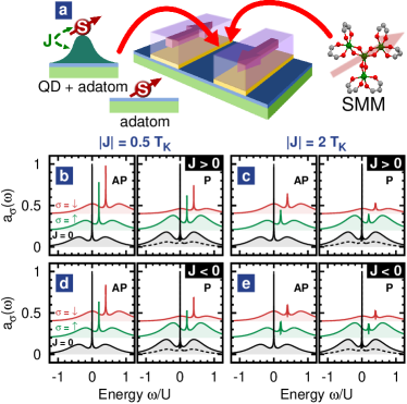
Figure 1: (Color online) (a) Schematic of a molecular quantum dot (magnetic molecule, magnetic adatom, or quantum dot exchange-coupled to a magnetic moment) coupled to two ferromagnetic electrodes. (b)-(e) Normalized spin-resolved orbital level (OL) spectral functions $a_{\sigma}(\omega)=\pi\Gamma_{\sigma}A_{\sigma}(\omega)$ in the antiparallel (left) and parallel (right part of each figure) magnetic configuration of electrodes for two different values of the exchange parameter $J$. The bottom curves (black) in each plot correspond to $J=0$, with the solid line referring to $\sigma=\uparrow$ and the dashed one to $\sigma=\downarrow$. To increase readability, for $J\neq 0$ the curves for $\sigma=\uparrow$ ($\sigma=\downarrow$) are shifted up and right by 0.2 (0.4). The parameters are: $S=2$, $U=1$ meV, $\varepsilon/U=-0.5$, $\Gamma/U\approx 0.075$, $D/U\approx 1.7\cdot 10^{-4}$, and $p=0.5$.

Model – We consider a generic model that includes essential features of such quantum objects like SMMs, magnetic adatoms, and quantum dots exchange coupled to local magnetic moments, see Fig. 1(a). These systems are referred to as magnetic quantum dots (MQDs). We assume that MQD is coupled to ferromagnetic leads whose magnetizations can form either parallel (P) or antiparallel (AP) configuration, while MQD’s magnetic easy axis is collinear with magnetic moments of the leads. We also assume that only a single orbital level (OL) of a MQD (lowest unoccupied molecular orbital of a SMM, atomic or quantum dot level) is directly coupled to the leads, while the corresponding magnetic core is coupled to the leads indirectly via exchange coupling to electrons in the local OL. The corresponding Hamiltonian reads Elste and Timm (2006); *Timm_PRB73/06; *Misiorny_PRB75/07; *Misiorny_PSS246/09; *Delgado_PRL104/10; M. Misiorny et al. (2009)

$$\mathcal{H}_{\textrm{MQD}}=-DS_{z}^{2}+\sideset{}{{}_{\sigma}}{\sum}\varepsilon\,n_{\sigma}+U\,n_{\uparrow}n_{\downarrow}-J\textbf{s}\cdot\textbf{S},$$ (1)

with $S_{z}$ denoting the $z$th component of the MQD’s core spin operator $\bm{S}$, and $D$ being the uniaxial anisotropy constant of the MQD. The operator $n_{\sigma}=c^{\dagger}_{\sigma}c_{\sigma}$, where $c_{\sigma}^{\dagger}(c_{\sigma})$ creates (annihilates) an electron of energy $\varepsilon$ in the OL, whereas $U$ denotes the Coulomb energy of two electrons occupying the OL. Energy (and therefore occupation) of this level can be controlled by an external gate voltage. Finally, the last term accounts for exchange coupling between the MQD’s magnetic core and electrons in the OL, with $\textbf{s}=(1/2)\sum_{\sigma\sigma^{\prime}}c_{\sigma}^{\dagger}\bm{\sigma}_{\sigma\sigma^{\prime}}c_{\sigma^{\prime}}$ and $\bm{\sigma}\equiv(\sigma^{x},\sigma^{y},\sigma^{z})$ denoting the Pauli matrices.

Method – To accurately address the problem of transport through MQDs in the strong coupling regime, we use the Wilson’s numerical renormalization group (NRG) method K.G. Wilson (1975). The NRG Hamiltonian of the full system can be then written as A.C. Hewson (1997); *Bulla_RevModPhys80/08

$$\mathcal{H}=\mathcal{H}_{\textrm{MQD}} +\sideset{}{{}_{\sigma}}{\sum}\sqrt{\Gamma_{\sigma}/(\pi\rho)}\big{[}c_{\sigma}^{\dagger}f_{0\sigma}+f_{0\sigma}^{\dagger}c_{\sigma}\big{]}$$

$$+\sideset{}{{}_{\sigma,n=0}^{\infty}}{\sum}t_{n}\big{[}f_{n\sigma}^{\dagger}f_{n+1\sigma}+f_{n+1\sigma}^{\dagger}f_{n\sigma}\big{]},$$ (2)

where $f_{n\sigma}$ ($f_{n\sigma}^{{\dagger}}$) represents the $n$th site of the Wilson’s chain (last term of $\mathcal{H}$) and $t_{n}$ denotes the hopping matrix element between neighboring sites of the chain. The second term of the NRG Hamiltonian stands for the coupling between the MQD and conduction electrons. Here, we use the flat band approximation, with the density of states $\rho=1/(2\mathfrak{D})$, where $\mathfrak{D}$ is the band half-width. The effect of ferromagnetic leads is then determined by the hybridization function $\Gamma_{\sigma}=\Gamma_{\rm L\sigma}+\Gamma_{\rm R\sigma}$ J. Martinek et al. (2003); *Sindel_PRB76/07, where $\Gamma_{r\sigma}$ is the coupling to the $r$th lead. When assuming left-right symmetry, the resultant coupling in the AP magnetic configuration does not depend on spin, $\Gamma_{\uparrow(\downarrow)}^{\textrm{AP}}=\Gamma$, and the system behaves then as being coupled to nonmagnetic leads. This is not the case in the P configuration where, $\Gamma_{\uparrow(\downarrow)}^{\textrm{P}}=\Gamma(1\pm p)$, with $p$ being the spin polarization of the leads and $\Gamma=(\Gamma_{\uparrow}+\Gamma_{\downarrow})/2$. By solving Hamiltonian (Interplay of the Kondo Effect and Spin-Polarized Transport in Magnetic Molecules, Adatoms and Quantum Dots) iteratively, we are able to determine static and dynamic quantities, basically at arbitrary energy R. Bulla et al. (2008). Transport properties of a MQD are then determined from the spectral function of the OL, $A_{\sigma}(\omega)=-\frac{1}{\pi}\textrm{Im}\{G^{\rm R}_{\sigma}(\omega)\}$, where $G^{\rm R}_{\sigma}(\omega)$ is the Fourier transform of the retarded Green’s function, $G_{\sigma}^{\rm R}(t)=-i\Theta(t)\langle\{c_{\sigma}(t),c_{\sigma}^{\dagger}(0)\}\rangle$.

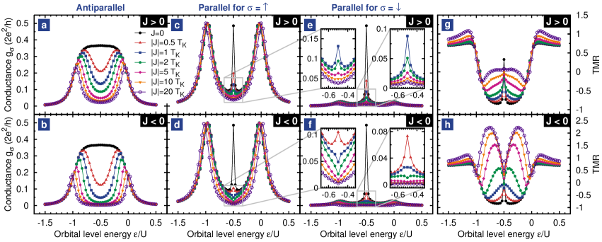
Figure 2: (Color online) (a)-(f) Dependence of the linear conductance $g_{\sigma}$ on the OL energy $\varepsilon$ for indicated values of the exchange parameter $J$ in the antiparallel (a)-(b) and parallel (c)-(f) magnetic configuration. Figures (g) and (h) show the corresponding TMR. Top panel represents the case of ferromagnetic ($J>0$) coupling between electrons in the OL and MQD’s magnetic core, whereas the bottom one corresponds to the antiferromagnetic ($J<0$) coupling. Parameters as in Fig. 1.

Spectral functions – The zero-temperature spin-resolved spectral functions $A_{\sigma}(\omega)$ of a singly occupied OL are shown in Figs. 1(b)-(e) for the P and AP configurations and for $\varepsilon=-U/2$. To begin with, we note that in the AP configuration the effective coupling is the same for both spin orientations. This is, however, opposite to the P configuration where an effective spin splitting of the OL due to spin-dependent coupling to the leads (effective exchange field) occurs J. Martinek et al. (2003). This exchange field depends on the position of the OL as $\delta\varepsilon_{\rm exch}\sim\ln|\varepsilon/(\varepsilon+U)|$. Consequently, the splitting will generally suppress the Kondo effect, except for the case of particle-hole symmetry point $\varepsilon=-U/2$ (shown in Fig. 1) where $\delta\varepsilon_{\rm exch}\to 0$. Therefore, for $\omega\lesssim T_{\rm K}$, where $T_{\rm K}$ is the Kondo temperature , the spectral functions in both configurations display a clear Kondo-Abrikosov-Suhl resonance at the Fermi level.

When considering the effect of finite exchange interaction $J$, one should note that there are two competing interactions corresponding to the energy scales set by $J$ and $T_{\textrm{K}}$. When $|J|<T_{\textrm{K}}$, the system then tends to lower its energy by $T_{\textrm{K}}$ due to formation of the many-body Kondo state. However, once $|J|>T_{\textrm{K}}$, it becomes energetically more favorable for an electron in the OL to hybridize with the core spin $S$ instead of free electrons in the leads. Thus, the resonant peak at the Fermi level will not develop in such a case. In Figs. 1(b)-(e) we show the spectral functions corresponding to both ferromagnetic ($J>0$) and antiferromagnetic ($J<0$) exchange couplings. It can be clearly seen that the Kondo effect becomes suppressed by the exchange coupling $J$, and this suppression is stronger for antiferromagnetic coupling. Actually, full suppression appears when $|J|\gtrsim T_{\textrm{K}}$.

Linear conductance – The spectral functions determine the linear conductance $g_{\sigma}$: $g_{\uparrow(\downarrow)}^{\textrm{AP}}=(e^{2}/h)(1-p^{2})\pi\Gamma A_{\uparrow(\downarrow)}^{\textrm{AP}}(0)$ for the antiparallel configuration, and $g_{\uparrow(\downarrow)}^{\textrm{P}}=(e^{2}/h)(1\pm p)\pi\Gamma A_{\uparrow(\downarrow)}^{\textrm{P}}(0)$ for the parallel one, where $A^{\rm P/AP}_{\sigma}(0)$ is the spectral function in the P/AP configuration for $\omega=0$. The linear conductance as a function of the OL energy is shown in Figs. 2(a)-(f) for different values of $J$. First, for $|J|\ll T_{\rm K}$ we recover results known for single-level quantum dots M.-S. Choi et al. (2004). For the AP magnetic configuration one observes then an enhanced conductance due to the Kondo state when the orbital level is singly occupied. The conductance is then given by, $g_{\uparrow(\downarrow)}^{\textrm{AP}}=(e^{2}/h)(1-p^{2})$, i.e. it is reduced by a polarization-dependent factor $(1-p^{2})=3/4$, as compared to the conductance quantum, see Figs. 2(a,b) and also Figs. 3(a,b) for $|J|/T_{\textrm{K}}\ll 1$. In the P configuration, in turn, the Kondo effect is suppressed due to effective spin splitting of the OL J. Martinek et al. (2003), except for $\varepsilon=-U/2$ where a sharp peak occurs and the Kondo effect is restored.

When $J\neq 0$, the Kondo anomaly in conductance becomes gradually suppressed with increasing $|J|$, and this suppression is faster for $J<0$ than for $J>0$. This behavior is a consequence of a difference in quantum states taking part in formation of the Kondo state for $J<0$ and $J>0$. First, the ground state energy $E_{\rm GS}$ of a singly-occupied bare MQD is lower for $J<0$ than for $J>0$, $E_{\rm GS}^{\rm AF}<E_{\rm GS}^{\rm F}$, while the energies of virtual states corresponding to empty and doubly occupied OL are independent of $J$. Second, the singly occupied MQD’s ground state for $J<0$ involves a superposition of both electronic spin states ‘up’ and ‘down’, which is not the case for $J>0$. Consequently, the cotunneling processes driving the Kondo effect for $J<0$ are suppressed more effectively than for $J>0$, and this behavior is clearly visible in the linear conductance, see Figs. 2(a,b). When the Kondo peak becomes suppressed, only two main resonances appear in the conductance, whose position depends on $J$: for $J>0$ they appear at $\varepsilon=JS/2$ and $\varepsilon=-JS/2-U$, while for $J<0$ their position depends linearly on $J$ and also weakly on $D$ M. Misiorny et al. (2009). It is also interesting to note that in the P configuration the resonance peaks are almost exclusively due to spin-up conductance $g^{\rm P}_{\uparrow}$, see Figs. 2(c-f). This is related to the fact that spin-up electrons are the majority ones in both the left and right lead and thus tunneling of spin-up electrons is favored, irrespective of $J$. The explicit dependence of the conductance on $J$ is shown in Figs. 3(a,b).

Tunnel magnetoresistance – The effects associated with exchange coupling $J$ are also pronounced in TMR, $\textrm{TMR}=(g^{\textrm{P}}-g^{\textrm{AP}})/g^{\textrm{AP}}$ with $g^{\rm P/AP}\equiv\sum_{\sigma}g^{\rm P/AP}_{\sigma}$, see Figs. 2(g)-(h). For $|J|\ll T_{\textrm{K}}$, the conductance in the Kondo regime is generally larger in the AP configuration than that in the P one, $g^{\rm AP}>g^{\rm P}$, leading to negative TMR in major part of the Coulomb blockade regime, except for $\varepsilon\approx-U/2$, when $g^{\rm AP}<g^{\rm P}$, and TMR is positive. When $|J|$ increases, the Kondo peak in AP configuration becomes suppressed too, and positive TMR in the blockade regime is restored. Since the suppression of $g^{\rm AP}$ is more pronounced for $J<0$, the corresponding TMR in the Kondo regime is larger for $J<0$ than for $J>0$. Moreover, TMR for $J<0$ significantly exceeds the corresponding Julliere’s value, $2p^{2}/(1-p^{2})$ ($=2/3$ for assumed parameters) Julliere (1975). On the other hand, for empty or doubly occupied OL, where transport is mainly determined by elastic cotunneling processes, one always finds $g^{\rm P}>g^{\rm AP}$ with TMR approaching the Julliere’s value.

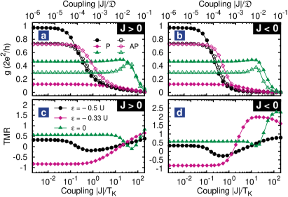
Figure 3: (Color online) Conductance $g=\sum_{\sigma}g_{\sigma}$ (a,b) and TMR (c,d) in the parallel (P) and antiparallel (AP) configurations as a function of the exchange parameter $J$ for indicated values of the OL energy $\varepsilon$. The dashed vertical line indicates the Kondo temperature. Other parameters as in Fig. 1.

The explicit variation of the spin-dependent conductance and the corresponding TMR with the parameter $J$ is shown in Fig. 3 for different values of $\varepsilon$. When $\varepsilon=-U/2$ and $|J|\rightarrow 0$, $\textrm{TMR}\approx p^{2}/(1-p^{2})$. In turn, as $|J|$ grows to energies corresponding to the Kondo temperature, $|J|\approx T_{\rm K}$, TMR reaches a minimum, where it takes negative values. Further growth of $|J|$ above $T_{\textrm{K}}$ is then accompanied by a significant increase in TMR, especially for $J<0$. In the Coulomb blockade regime with $\varepsilon\neq-U/2$, TMR is negative and constant for $|J|<T_{\rm K}$, and starts increasing when $|J|>T_{\rm K}$ to reach large positive values for $|J|\gg T_{\rm K}$ in the case of $J<0$, see Fig. 3(b). In turn, at resonance, $\varepsilon=0$, TMR is positive and constant and only slightly decreases when $|J|\approx\Gamma$, where a local minimum develops due to the dependence of resonance energies on $J$.

The uniaxial anisotropy $D$ modifies the energy spectrum and electron states of MQD, and therefore has a significant influence on the Kondo state J. J. Parks et al. (2010), which can be observed in the behavior of $g$ and TMR. In Fig. 4 we show the $\varepsilon$-dependence of TMR for different values of the anisotropy constant $D$. We note that the effects due to variation of $D$ are mainly visible in the Kondo regime, while outside the Coulomb blockade TMR is rather independent of $D$. Moreover, this effect is more pronounced for $J<0$ than for $J>0$. This is because magnetic anisotropy changes quantum states responsible for the Kondo effect, suppressing the difference in TMR for $J<0$ and $J>0$, see Fig. 4(b).

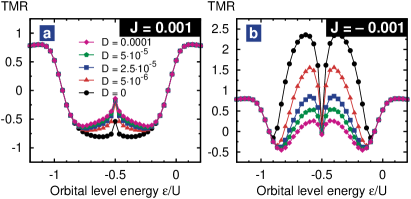
Figure 4: (Color online) Influence of the molecule’s magnetic anisotropy $D$ on TMR for the ferromagnetic (a) and antiferromagnetic (b) exchange coupling $J$. Parameters are the same as in Fig. 1 with $|J|=2T_{\textrm{K}}$.

Conclusions – Using numerical renormalization group method we have studied spin-dependent transport through a localized orbital level coupled directly to ferromagnetic leads and exchange-coupled to a magnetic core. We have shown that there is a competition between interactions corresponding to two energy scales: the Kondo temperature $T_{\textrm{K}}$ and exchange coupling $J$. The linear conductance becomes suppressed when $|J|\gtrsim T_{\textrm{K}}$ and this suppression is more pronounced in the case of antiferromagnetic coupling $J$. Moreover, $J$ also has a significant influence on TMR, which displays a nonmonotonic dependence on $J$ with a minimum for $|J|\approx T_{\rm K}$ and may be greatly enhanced when $J<0$ as compared to the case of $J>0$.

M.M acknowledges the hospitality of Lehrstuhl J. von Delft. I.W. acknowledges support from the Alexander von Humboldt Foundation and funds of the Polish Ministry of Science and Higher Education as research project for years 2008-2010.

References

- C. Joachim et al. (2000) C. Joachim et al., Nature, 408, 541 (2000).
- S.J. Tans et al. (1998) S.J. Tans et al., Nature, 393, 49 (1998).
- H. Park et al. (2000) H. Park et al., Nature, 407, 57 (2000).
- P.G. Piva et al. (2005) P.G. Piva et al., Nature, 435, 658 (2005).
- Heath and Ratner (2003) J. Heath and M. Ratner, Phys. Today, 56, 43 (2003).
- Bogani and Wernsdorfer (2008) L. Bogani and W. Wernsdorfer, Nature Mater., 7, 179 (2008).
- J.E. Green et al. (2007) J.E. Green et al., Nature, 445, 414 (2007).
- M. Mannini et al. (2009) M. Mannini et al., Nature Mater., 8, 194 (2009).
- S. Loth et al. (2010) S. Loth et al., Nature Phys., 6, 340 (2010).
- C.F. Hirjibehedin et al. (2007) C.F. Hirjibehedin et al., Science, 317, 1199 (2007).
- A.F. Otte et al. (2008) A.F. Otte et al., Nature Phys., 4, 847 (2008).
- Gatteschi et al. (2006) D. Gatteschi, R. Sessoli, and J. Villain, Molecular nanomagnets (Oxford University Press, New York, 2006).
- H.B. Heersche et al. (2006) H.B. Heersche et al., Phys. Rev. Lett., 96, 206801 (2006).
- M.-H. Jo et al. (2006) M.-H. Jo et al., Nano Lett., 6, 2014 (2006).
- S. Voss et al. (2008) S. Voss et al., Phys. Rev. B, 78, 155403 (2008).
- A.S. Zyazin et al. (2010) A.S. Zyazin et al., Nano Lett., 10, 3307 (2010).
- Elste and Timm (2006) F. Elste and C. Timm, Phys. Rev. B, 73, 235305 (2006).
- Timm and Elste (2006) C. Timm and F. Elste, Phys. Rev. B, 73, 235304 (2006).
- Misiorny and Barnaś (2007) M. Misiorny and J. Barnaś, Phys. Rev. B, 75, 134425 (2007).
- Misiorny and Barnaś (2009) M. Misiorny and J. Barnaś, Phys. Stat. Sol. B, 246, 695 (2009).
- F. Delgado et al. (2010) F. Delgado et al., Phys. Rev. Lett., 104, 026601 (2010).
- M. Misiorny et al. (2009) M. Misiorny et al., Phys. Rev. B, 79, 224420 (2009).
- H.-Z. Lu et al. (2009) H.-Z. Lu et al., Phys. Rev. B, 79, 174419 (2009).
- S. Barraza-Lopez et al. (2009) S. Barraza-Lopez et al., Phys. Rev. Lett., 102, 246801 (2009).
- M .Misiorny et al. (2010) M .Misiorny et al., Europhys. Lett., 89, 18003 (2010).
- J. J. Parks et al. (2010) J. J. Parks et al., Science, 328, 1370 (2010).
- C. Romeike et al. (2006) C. Romeike et al., Phys. Rev. Lett., 96, 196601 (2006a).
- C. Romeike et al. (2006) C. Romeike et al., Phys. Rev. Lett., 97, 206601 (2006b).
- M.N. Leuenberger and E.R. Mucciolo (2006) M.N. Leuenberger and E.R. Mucciolo, Phys. Rev. Lett., 97, 126601 (2006).
- Gonzalez and Leuenberger (2007) G. Gonzalez and M. Leuenberger, Phys. Rev. Lett., 98, 256804 (2007).
- G. Gonzalez et al. (2008) G. Gonzalez et al., Phys. Rev. B, 78, 054445 (2008).
- K.G. Wilson (1975) K.G. Wilson, Rev. Mod. Phys, 47, 773 (1975).
- A.C. Hewson (1997) A.C. Hewson, The Kondo problem to heavy fermions (Cambridge University Press, 1997).
- R. Bulla et al. (2008) R. Bulla et al., Rev. Mod. Phys., 80, 395 (2008).
- J. Martinek et al. (2003) J. Martinek et al., Phys. Rev. Lett., 91, 127203 (2003).
- M. Sindel et al. (2007) M. Sindel et al., Phys. Rev. B, 76, 45321 (2007).
- Note (1) The system’s Kondo temperature defined as half-width of the total spectral function in the antiparallel configuration for is .
- M.-S. Choi et al. (2004) M.-S. Choi et al., Phys. Rev. Lett., 92, 56601 (2004).
- Julliere (1975) M. Julliere, Phys. Lett. A, 54, 225 (1975).