On the horoboundary and the geometry of rays
of negatively curved manifolds.

1 Introduction

The problem of understanding the geometry and dynamics of geodesics and rays (i.e. distance-minimizing half-geodesics) on Riemannian manifolds dates back at least to Hadamard [20], who started to study the qualitative behaviour of geodesics on nonpositevely curved surfaces of $\mathbb{R}^{3}$. In particular, he first distinguished between different kinds of ends on such surfaces, and introduced the notion of asymptote, which we shall be concerned about in this paper.
Half a century later, in his seminal book [11], Busemann introduced an amazingly simple notion for measuring the “angle at infinity” between rays (now known as the Busemann function) as a tool to develop a theory of parallels on geodesic spaces. The Busemann function of a ray $\alpha$ is the two-variables function

$$B_{\alpha}(x,y)=\lim_{t\rightarrow+\infty}d(x,\alpha(t))-d(\alpha(t),y)$$

and played an important role (far beyond the purposes of his creator) in the study of complete noncompact Riemannian manifolds.
It has been used to derive fundamental results in nonnegative curvature such as Cheeger-Gromoll-Meyer’s Soul Theorem or Toponogov’ Splitting Theorem ([36]), in the function theory of harmonic and noncompact symmetric spaces ([1], [22]), and has a special place in the geometry of Hadamard spaces and in the dynamics of Kleinian groups. The main reason for this place is that any simply connected, nonpositively curved space $X$ (a Hadamard space) has a natural, “visual” compactification whose boundary $X(\infty)$ is easily described in terms of asymptotic rays; and, when $X$ is given a discrete group $G$ of motions, the Busemann functions of rays appear as the densities at infinity of the Patterson-Sullivan measures of $G$ ([35], [39]).

The simple visual picture of the compactification of a Hadamard space unfortunately breaks down for general, non-simply connected manifolds: but Busemann functions (more precisely, their direct generalizations known as horofunctions) have inspired Gromov to define a natural, universal compactification (the horofunction compactification), whose properties however are more difficult to describe. The aim of this paper is to investigate how far the visual description of this boundary and the usual properties of rays carry over in the negatively curved, non-simply connected case, and to stress the main differences.

Let us start by describing a first, naïf approach to the problem of finding a “good” geometric compactification of a general complete Riemannian manifold. The first idea is to add all “asymptotic directions” to the space, similarly to $\mathbb{E}^{n}$ which can be compactified as the closed ball $B^{n}=\mathbb{E}^{n}\cup S^{n}$ by adding the set of all oriented half-lines modulo (orientation-preserving) parallelism. Now, on a general Riemannian manifold we have at least two elementary notions of asymptoticity for rays $\alpha,\beta:\mathbb{R}^{+}\rightarrow X$ with, respectively, origins $a,b$:

$\bullet$ Distance Asymptoticity: we say that $d_{\infty}(\alpha,\beta)\!<\!\infty$ if $\sup_{t}d(\alpha(t),\beta(t))\!<\!\infty$,
and then we say that $\alpha$ and $\beta$ are distance-asymptotic (or, simply, asymptotic);

$\bullet$ Visual Asymptoticity: we say that $\alpha$ tends visually to $\beta$, and write it $\alpha\succ\beta$, if there exist minimizing geodesic segments $\beta_{n}=[b,\alpha(t_{n})]$ such that $\beta_{n}\rightarrow\beta$ (i.e. the angle $\angle\beta,\beta_{n}\rightarrow 0$); it is also current to say in this case that $\beta$ is a coray to $\alpha$ ($\beta\prec\alpha)$, following Busemann [11]. Then, we say that $\alpha$ and $\beta$ are visually asymptotic if $\alpha\succ\beta$ and $\beta\succ\alpha$ ($\alpha\prec\succ\beta$).

It is classical that these two notions of asymptoticity coincide for Hadamard spaces. For a Hadamard space $X$ one then defines the visual boundary $X(\infty)$ as the set of rays ${\cal R}(X)$ modulo asymptoticity, gives to $\overline{X}=X\cup X(\infty)$ a natural topology which coincides on $X$ with the original one and makes of it a compact metrizable space: we will refer to $\overline{X}$ as to the visual compactification of $X$ (cp. [14] and Section §3.1).

The idea of proceeding analogously for a general Riemannian manifold is tempting but disappointing. First, besides the case of Hadamard spaces, the relation $\prec$ is known to be generally not symmetric, and the relation $\prec\succ$ is not an equivalence relation (exceptly for rays having the same origin, as Theorem 16 shows). Some indirect examples of the asymmetry can be found in literature for surfaces with variable curvature [21], or for graphs [34]. We shall give in Section §6 an example of hyperbolic surface (the Asymmetric Hyperbolic Flute) which makes evident the general asymmetry of the coray relation, which can be interpreted in terms of the geometrical asymmetry of the surface itself. More difficult is to exhibit a case where $\prec\succ$ is not an equivalence relation: Theorem 16 and Example 44(a) (the Hyperbolic Ladder) will make it explicit. The problem that visual asymptoticity is not an equivalence relation has been by-passed by some authors ([26], [29]) by taking the equivalence relation generated by $\prec$ (this means partitioning all the corays to some ray $\alpha$ into maximal packets all of which contain only rays corays to each other): this exactly coincides with taking rays with the same Busemann function (see [23] and Section §2), which explains the original interest of Busemann in this function. We will see in §2.2 that the condition $B_{\alpha}=B_{\beta}$ geometrically simply means that we can see $\alpha(t)$ and $\beta(t)$, for $t\gg 0$, under a same direction from any point of the manifold.

Secondly, distance and visual asymptoticity (even in this stronger form) are strictly distinct relations on general manifolds: there exist rays staying at bounded distance from each other having different Busemann functions, and also, more surprisingly, diverging rays defining the same Busemann function. This already happens in constant negative curvature:

Theorem 1

(The Hyperbolic Ladder 44 & The Symmetric Hyperbolic Flute 41)

There exist hyperbolic surfaces $S_{1},S_{2}$ and rays $\alpha_{i},\alpha_{i}^{\prime}$ on $S_{i}$ such that:
(i) $d_{\infty}(\alpha_{1},\alpha_{1}^{\prime})<\infty$ but $B_{\alpha_{1}}\neq B_{\alpha_{1}^{\prime}}$;
(ii) $B_{\alpha_{2}}=B_{\alpha_{2}^{\prime}}$ but $d_{\infty}(\alpha_{2},\alpha_{2}^{\prime})=+\infty$.

Worst, trying to define a boundary $X^{d}(\infty)$ or $X^{v}(\infty)$ from ${\cal R}(X)$ by identifying rays under any of these asymptotic relations generally leads to a non-Hausdorff space, because these relations are not closed (with ${\cal R}(X)$ endowed of the topology of uniform convergence on compacts):

Theorem 2

(The Twisted Hyperbolic Flute 42)

There exist a hyperbolic surface $X$ and rays $\alpha_{n}\rightarrow\alpha$ on $X$ such that:
(i) $d_{\infty}(\alpha_{n},\alpha_{m})<\infty$ but $d_{\infty}(\alpha_{n},\alpha)=\infty$ for all $n,m$;
(ii) $B_{\alpha_{n}}=B_{\alpha_{m}}$ but $B_{\alpha_{n}}\neq B_{\alpha}$ for all $n,m$.

This prevents doing any reasonable measure theory (e.g. Patterson-Sullivan theory) on any compactification built out of $X^{d}(\infty)$, $X^{v}(\infty)$. A remarkable example where this problems occurs is the Teichmuller space ${\cal T}_{g}$ which, endowed with the Teichmuller metric, has a non-Hausdorff visual boundary for $g\geq 2$ [27].

Gromov’s idea of compactification overrides the difficulty of using asymptotic rays, by considering the topological embedding

$$b:X\hookrightarrow C(X)/\mathbb{R}\;\;\;P\mapsto[d(P,\cdot)]$$

of any Riemannian manifold $X$ in the space of real continuous functions on $X$ (with the uniform topology), up to additive constants. He defines $\overline{X}$ as the closure of $b(X)$ in $C(X)/\mathbb{R}$, and its boundary as $\partial X=\overline{X}-b(X)$, obtaining a compact, Hausdorff (even metrizable) space where $X$ sits in. We will call $\overline{X}$ the horofunction compactification of $X$, and $\partial X$ the horoboundary of $X$.
The points of $\partial X$ are commonly called horofunctions; Busemann functions then naturally arise as particular horofunctions: actually, for points of $X$ diverging along a ray $P_{n}=\alpha(n)$ we have that

$$b(P_{n})=[d(P_{n},\cdot)]=[d(x,P_{n})-d(P_{n},\cdot)]\longrightarrow[B_{\alpha}(x,\cdot)]$$

in $C(X)/\mathbb{R}$, cp. Section §2 for details. Accordingly, the Busemann map

$$B:{\cal R}(X)\rightarrow\partial X$$

is the map which associates to each ray the class of its Busemann function. For Hadamard manifolds, it is classical that $B$ induces a homeomorphism between the visual boundary $X(\infty)$ and the horoboundary $\partial X$ (cp. §2).

The properties of the Busemann map for general nonpositively curved Riemannian manifolds will be the second object of our interest in this paper. The main questions we address are:

(a) the Busemann Equivalence: i.e., when do the Busemann functions of two distinct rays coincide?

Actually, the equivalence relation generated by the coray relation is difficult to test in concrete examples. In Section §4 we discuss several notions of equivalence of rays related to the Busemann equivalence; then we give a characterization (Theorem 28) of the Busemann equivalence for rays on quotients of Hadamard spaces, in terms of the points at infinity of their lifts, which we call weak $G$-equivalence. For rays with the same origin, it can be stated as follows:

Criterium 3

Let $X=G\backslash\tilde{X}$ be a regular quotient of a Hadamard space.
Let $\alpha,\beta$ be rays based at $o$, with lifts $\widetilde{\alpha},\widetilde{\beta}$ from $\tilde{o}\in\tilde{X}$, and let $H_{\tilde{\alpha}},H_{\widetilde{\beta}}$ be the horoballs through $\tilde{o}$ centered at the respective points at infinity $\widetilde{\alpha}^{+},\widetilde{\beta}^{+}$. Then:

$$B_{\alpha}\!=\!B_{\beta}\Leftrightarrow\exists\,(g_{n}),(h_{n})\!\in\!G\mbox{ such that }\left\{\!\begin{array}[]{l}g_{n}\widetilde{\alpha}^{+}\rightarrow\beta^{+}\\ \!\!d(g_{n}^{-1}\tilde{o},H_{\tilde{\alpha}})\rightarrow 0\end{array}\right.\!\!\mbox{and}\left\{\!\begin{array}[]{l}h_{n}\widetilde{\beta}^{+}\rightarrow\alpha^{+}\\ \!\!d(h_{n}^{-1}\tilde{o},H_{\tilde{\beta}})\rightarrow 0\end{array}\right.$$

This reduces the problem of the Busemann equivalence for rays $\alpha,\beta$ on quotients of a Hadamard space to the problem of approaching the limit points (of their lifts) $\widetilde{\alpha}^{+},\widetilde{\beta}^{+}$ with sequences $g_{n}\widetilde{\beta}^{+}$, $h_{n}\widetilde{\alpha}^{+}$ in the respective orbits, keeping at the same time control of the dynamics of the inverses $g_{n}^{-1},h_{n}^{-1}$.

(b) the Surjectivity of the Busemann map: i.e., is any point in the horoboundary of $X$ equal to the Busemann function of some ray?

In this perspective, it is natural to extend the Busemann map $B$ to the set $q{\cal R}(X)$ of quasi-rays (i.e. half-lines $\alpha:R^{+}\rightarrow X$ which are only almost-minimizing, cp. Definition 8); we then call Busemann boundary ${\cal B}X=B(q{\cal R}(X))$. The problem whether ${\cal B}X=\partial X$ has been touched by several authors for surfaces with finitely generated fundamental group (cp. [37] and [44]). In [44] there are examples of a non-negatively curved surface admitting horofunctions which are not in ${\cal B}X$, and even of surfaces where the set of Busemann functions of rays emanating from one point is different from that of rays emanating from another point. This explains our interest in considering rays with variable initial points, instead of keeping the base point fixed once and for all.

In [25] Ledrappier and Wang start developing the Patterson-Sullivan theory on non-simply connected manifolds, and the question whether an orbit accumulates to a limit point which is a true Busemann function naturally arises; the Theorem below shows that, in this context, Patterson-Sullivan theory must take into account limit points which are not Busemann functions, and that some paradoxical facts already happen in the simplest cases:

Theorem 4

(The Hyperbolic Ladder 44)

There exists a Galois covering $X\rightarrow\Sigma_{2}$ of a hyperbolic surface of genus $2$, with automorphism group $\Gamma\cong\mathbb{Z}$, such that:

(i) ${\cal B}X$ consists of 4 points, while $\partial X$ consists of a continuum of points;

(ii) the limit set $L\Gamma=\overline{\Gamma x_{0}}\cap\partial X$ depends on the choice of the base point $x_{0}$, and for some $x_{0}$ it is included in $\partial X-{\cal B}X$.

The problem of surjectivity and the interest in finding Busemann points in the horoboundary seems to have been revitalized due to recent work on Hilbert spaces (cp. [41], [42]), on the Heisenberg group [24], on word-hyperbolic groups and general Cayley graphs (cp. [6], [43]). A construction similar to that of Theorem 4 is discussed in [10] as an example where the boundary of a Gromov-hyperbolic space does not coincide with the horoboundary (notice however that the notion of boundary for Gromov-hyperbolic spaces differs from ${\cal B}X$, as it is defined up to a bounded function).

(c) the Continuity of the Busemann map: i.e., how does the Busemann functions change with respect to the initial direction of rays?

This is crucial to understand the topology of the horofunction compactification and, beyond the simply connected case, it has not been much investigated in literature so far. Busemann himself seemed to exclude it in full generality.
We shall see that, in general, the dependence from the initial conditions is only lower-semicontinuous:

Theorem 5

(Proposition 30 & The Twisted Hyperbolic Flute 42)

Let $X=G\backslash\tilde{X}$ be the regular quotient of a Hadamard space.
(i) for any sequence of rays $\alpha_{n}\rightarrow\alpha$ we have $\lim_{n\rightarrow\infty}B_{\alpha_{n}}\geq B_{\alpha}$;

(ii) there exists $X=G\backslash\mathbf{H}^{2}$ and rays $\alpha_{n}\rightarrow\alpha$ such that $\lim_{n\rightarrow\infty}B_{\alpha_{n}}>B_{\alpha}$. (Convergence of rays is always meant uniform on compacts.)

The example of the Twisted Hyperbolic Flute 42 is the archetype where a jump between $\lim_{n\rightarrow\infty}B_{\alpha_{n}}$ and $B_{\alpha}$ occurs; we will explain geometrically –actually, we produce, the discontinuity in terms of a discontinuity in the limit of the maximal horoballs associated to the $\alpha_{n}$ in the universal covering, cp. Definition 20 and Remark 43. Interpreting $e^{-B_{\alpha}(o,\cdot)}$ as a reparametrized distance to the point at infinity of $\alpha$, the jump can be seen as a hole suddenly appearing in a limit direction of a hyperbolic sky.
We stress the fact that the problem of continuity makes sense only for rays $\alpha_{n}$ (i.e. whose velocity vectors yield minimizing directions): it is otherwise easy to produce a discontinuity in the Busemann function of a sequence of quasi-rays tending to some limit curve which is not minimizing (and for which the Busemann function may be not defined), cp. Example 29 in §4 and the discussion therein.

It is noticeable that all the possible pathologies in the geometry of rays which we described above already occur for hyperbolic surfaces belonging to two basic classes: flutes and ladders, see Section §6. These are surfaces with infinitely generated fundamental group whose topological realizations are, respectively, infinitely-punctured spheres and $\mathbb{Z}$-coverings of a compact surface of genus $g\geq 2$:

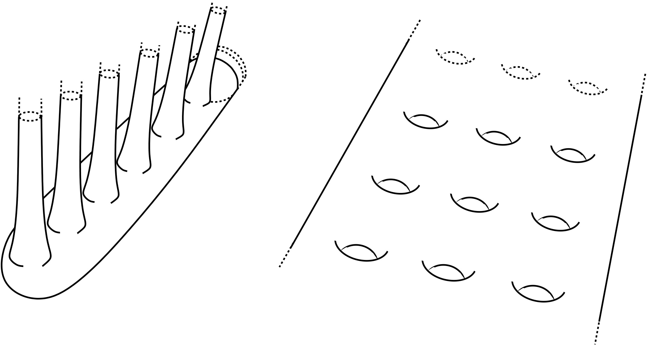
Figure 1: Geometric realization of flutes and ladders

On the other hand, limiting ourselves to the realm of surfaces with finitely generated fundamental group, all the above pathologies disappear and we recover the familiar picture of rays on Hadarmard manifolds. More generally, in Section §5 we will consider properties of rays and the Busemann map for geometrically finite manifolds: these are the geometric generalizations, in dimension greater than $2$, of the idea of negatively curved surface with finite connectivity (i.e. finite Euler-Poincaré characteristic). The precise definition of this class and much of these manifolds is due to Bowditch [8]; we will summarize the necessary definitions and properties in Section §5. We will prove:

Theorem 6

(Propositions 33, 34, 35, 36 & Corollary 37)

Let $X=G\backslash\tilde{X}$ be a geometrically finite manifold:

(i) every quasi-ray on $X$ is finally a ray (i.e. it is a pre-ray, cp. Definition 8);

(ii) $d_{\infty}(\alpha,\beta)<\infty\;\Leftrightarrow\;B_{\alpha}=B_{\beta}\;\Leftrightarrow\;\alpha\prec\beta$ for rays $\alpha,\beta$ on $X$;

(iii) the Busemann map ${\cal R}(X)\rightarrow\partial X$ is surjective and continuous.

As a consequence, $X(\infty)={\cal R}(X)/_{(Busemann\;eq.)}$ is homeomorphic to $\partial X$ and:

$\bullet$ if dim$(X)=2$, $\overline{X}$ is a compact surface with boundary;

$\bullet$ if dim$(X)>2$, $\overline{X}$ is a compact manifold with boundary, with a finite number of conical singularities (one for each class of maximal parabolic subgroups of $G$).

In this regard, it is of interest to recall that the question whether any geometrically finite manifold has finite topology (i.e., is homeomorphic to the interior of a compact manifold with boundary) was asked by Bowditch in [8], and recently answered by Belegradek and Kapovitch, cp. [5]. However, Belegradek and Kapovitch’s proof yields a natural topological compactification whose boundary points are less related to the geometry of the interior than in the horofunction compactification. According to [5], any horosphere quotient is diffeomorphic to a flat Euclidean vector bundle over a compact base, so a parabolic end can be seen as the interior of a closed cylinder over a closed disk-bundle. On the other hand, in the horofunction compactification, a parabolic end is compactified as a cone over the Thom space of this disk-bundle (cp.Corollary 37&Example 38); one pays the geometric content of the horofunction compactification by the appearing of (topological) conical singularities.
The problem of relating the ideal boundary and the horoboundary for geometrically finite groups has also been considered in [22]; there, the authors prove that, in the case of arithmetic lattices of symmetric spaces, both compactifications coincide with the Tits compactification, and also discuss the relation with the Martin boundary.

Section §2 is preliminary: we report here some generalities about the Busemann functions and the coray relation.

From Section §3 on, we focus on nonpositively curved manifolds. We briefly recall the classical visual properties of rays on Hadamard spaces, and then we turn our attention to their quotients $X=G\backslash\tilde{X}$. The difference between rays and quasi-rays is deeply related with the different kind of points at infinity of their lift to $\tilde{X}$; that is why we review a dictionary between limit points of $G$ and corresponding quasi-rays on $X$. Then, we prove a formula (Theorem 24) expressing the Busemann function of a ray $\alpha$ on $X$ in terms of the Busemann function of a lift $\widetilde{\alpha}$ of $\alpha$ to $\tilde{X}$. We will use this formula to translate the Busemann equivalence in terms of the above mentioned weak $G$-equivalence; this turns out to be the key-tool for constructing examples having Busemann functions with prescribed behaviour.

In Section §4 we discuss the properties of the Busemann map on general quotients of Hadamard spaces; here we prove the Criterium 3 and the lower semicontinuity.

Section §5 is devoted to geometrically finite manifolds and to the proof of Theorem 6.

Finally, we collect in Section §6 the main examples of the paper (the Asymmetric, Symmetric and Twisted Hyperbolic Flute, and the Hyperbolic Ladder).

In the Appendix we report, for the convenience of the reader, proofs of those facts which are either classical, but essential to our arguments, or which we were not able to find easily in literature.

We will always assume that geodesics are parametrized by arc-length, and we will use the symbol $[p,q]$ for a minimizing geodesic segment connecting two points $p,q$. Moreover, we shall often use, in computations, the notations $x\apprle_{\epsilon}y$ for $x\leq y+\epsilon$ (respectively, $x\eqsim_{\epsilon}y$ for $|x-y|\leq\epsilon$) and abbreviate $d(x,y)$ with $xy$.

2 Busemann functions on Riemannian manifolds

2.1 Horofunctions and Busemann functions

Let $X$ be any complete Riemannian manifold (not necessarily simply connected). The horofunction compactification of $X$ is obtained by embedding $X$ in a natural way into the space $C(X)$ of real continuous functions on $X$, endowed with the $C^{0}$-topology (of uniform convergence on compact sets):

$$b:X\hookrightarrow C(X)\hskip 28.45274ptP\mapsto-d(P,\cdot)$$

then, defining $\overline{X}\doteq\overline{b(X)}$ and $\partial X\doteq\overline{X}-b(X)$.
An (apparently) more complicate version of this construction has the advantage of making the Busemann functions naturally appear as boundary points. For fixed $P$, define the horofunction cocycle as the function of $x,y$:

$$b_{P}(x,y)=d(x,P)-d(P,y)$$

then, consider the space of functions in $C(X)$ up to an additive costant (with the quotient topology) and the same map

$$b:X\rightarrow C(X)/\mathbb{R}\hskip 28.45274ptP\mapsto[-d(P,\cdot)]=[d(x,P)-d(P,\cdot)]=[b_{P}(x,\cdot)]$$

(which is independent from the choice of $x$). The following properties hold, in all generality, for any complete Riemannian manifold, and can be found, for instance, in [3] or [10]:

1) $b$ is a topological embedding, i.e. an injective map which is a homeomorphism when restricted to its image;

2) $\overline{X}$ is a compact, 2^nd-countable, metrizable space.

Definition 7

Horoboundary and horofunctions
The horofunction compactification of $X$ and the horoboundary of $X$ are respectively the sets $\overline{X}\doteq\overline{b(X)}$ and $\partial X\doteq\overline{X}-b(X)$. A horofunction is an element $\xi\in\partial X$, that is the limit of a sequence $[b_{P_{n}}]$, for $P_{n}\in X$ going to infinity; we will write $\xi=B_{(P_{n})}$.

Notice that, as $b_{P}(x,y)-b_{P}(x^{\prime},y)=b_{P}(x,x^{\prime})$ saying that $(P_{n})\rightarrow\xi\in\partial X$ is equivalent to saying that, for any fixed $x$, the horofunction cocycle $b_{P_{n}}(x,\cdot)$ converges uniformly on compacts for $n\rightarrow\infty$ (to a representative of $\xi$). Concretely, we see a horofunction $\xi=B_{(P_{n})}$ as a function of two variables $(x,y)$ satisfying:

(i) (cocycle condition) $\;\;B_{(P_{n})}(x,y)-B_{(P_{n})}(x^{\prime},y)=B_{(P_{n})}(x,x^{\prime})$

or, equivalently , $B_{(P_{n})}(x,x^{\prime})+B_{(P_{n})}(x^{\prime},y)=B_{(P_{n})}(x,y)$.

The following properties follow right from the definitions:

(ii) (skew-symmetry)       $B_{(P_{n})}(x,y)=-B_{(P_{n})}(y,x)$

(iii) (1-Lipschitz)           $B_{(P_{n})}(x,y)\leq d(x,y)$

(iv) (invariance by isometries) $\;\;B_{(gP_{n})}(gx,gy)=B_{(P_{n})}(x,y)\;\;\forall g\in Isom(X)$

(v) (continuous extension)   the cocycle $b_{P}(x,y)$ can be extended to a continuous function $B:X\times\overline{X}\times X\rightarrow\mathbb{R}$, i.e. $B_{\xi}(x,y)=\lim_{n\rightarrow\infty}b_{P_{n}}(x,y)$ if $(P_{n})\rightarrow\xi$;

(vi) (extension to the boundary) every $g\in Isom(X)$ naturally extends to a homeomorphism $g:\partial X\rightarrow\partial X$.

Now, the simplest way of diverging, for a sequence of points $\{P_{n}\}$ on an open manifold $X$, is to go to infinity along a geodesic. As we deal with non-simply connected manifolds, we shall need to distinguish between geodesics and minimizing geodesics:

Definition 8

Excess and quasi-rays

The length excess of a curve $\alpha$ defined on an interval $I$ is the number

$$\Delta(\alpha)=\sup_{t,s\in I}\ell(\alpha;t,s)-d(\alpha(t),\alpha(s))$$

that is the greatest difference between the length of $\alpha$ between two of its points, and their effective distance. Accordingly, we say that a geodesic $\alpha$ in a manifold $X$ is quasi-minimizing if $\Delta(\alpha)<+\infty$, and $\epsilon$-minimizing if $\Delta(\alpha)\leq\epsilon$.
A quasi-ray is a quasi-minimizing half-geodesic $\alpha:\mathbb{R}_{+}\rightarrow X$. For a quasi-ray $\alpha$ there are three possibilities:

$\bullet$ either $\alpha$ is minimizing (i.e. $\Delta(\alpha)=0$): then $\alpha$ is a true ray;

$\bullet$ or $\alpha|_{[t_{0},+\infty]}$ is minimizing for some $a>0$, an then we call $\alpha$ a pre-ray;

$\bullet$ or $\Delta(\alpha)<\infty$ but $\alpha|_{a,+\infty}$ is never minimizing, for any $a\in\mathbb{R}$; in this case, following [19], we call $\alpha$ a rigid quasi-ray.

We will denote by ${\cal R}(X)$ and $q{\cal R}(X)$ the sets of rays and quasi-rays of $X$ (resp. ${\cal R}_{o}(X)$ and $q{\cal R}_{o}(X)$ those with origin $o$), with the uniform topology given by convergence on compact sets.

There exist, in literature, examples of all three kinds of quasi-rays.
An enlightening example is the modular surface $X=PSL(2,\mathbb{Z})\backslash\mathbf{H}^{2}$ (though only an orbifold). $X$ has a 6-sheeted, smooth covering $\hat{X}=\Gamma(2)\backslash\mathbf{H}^{2}\rightarrow X$, with finite volume; the half-geodesics $\alpha$ of $\hat{X}$ with infinite excess are precisely the bounded geodesics and the unbounded, recurrent ones (those who come back infinitely often in a compact set); their lifts in the half-plane model of $\mathbf{H}^{2}$ correspond to the half-geodesics $\widetilde{\alpha}$ having extremity $\widetilde{\alpha}^{+}\in\mathbb{R}-\mathbb{Q}$ . Moreover, $\alpha$ is bounded if and only if $\widetilde{\alpha}^{+}$ is a badly approximated number (i.e. its continued fraction expansion is a sequence of bounded integers), see [12]. In this case, all half-geodesics $\alpha$ with $\Delta(\alpha)<\infty$ (corresponding to lifts $\widetilde{\alpha}$ with rational extremity) are minimizing after some time, i.e. they are pre-rays.
On the other hand, in [19] one can find examples and classification of rigid quasi-rays on particular (undistorted) hyperbolic flute surfaces.

For future reference, we report here some properties of the length excess:

Properties 9

Let $\alpha,\alpha_{k}:[0,+\infty]\rightarrow X$ curves with origins respectively $a$, $a_{k}$:

(i) if $\Delta(\alpha)<\infty$, then for every $\epsilon>0$ there exists $T_{\epsilon}\gg 0$ such that

$$\Delta(\alpha|_{[T_{\epsilon},+\infty]})\leq\epsilon\;\;\;\;\mbox{ and }\;\;\;\;\Delta(\alpha|_{[0,T_{\epsilon}]})\geq\Delta(\alpha)-\epsilon\;;$$

(ii) if $\alpha_{k}\rightarrow\alpha$ uniformly on compacts, then $\Delta(\alpha)\leq\liminf_{k\rightarrow\infty}\Delta(\alpha_{k})$.
In particular, any limit of minimizing geodesics segments is minimizing.

(iii) Assume now that the universal covering of $X$ is a Hadamard space.
If $\widetilde{\alpha}$ is a lift of $\alpha$ to $\tilde{X}$ with origin $\tilde{a}$, then:

$$\Delta(\alpha)=\lim_{t\rightarrow+\infty}d(\tilde{a},\widetilde{\alpha}(t))-d(a,\alpha(t))$$

Proof. (i) follows from the fact that the excess is increasing with the width of intervals. For (ii), pick $T_{\epsilon}$ as in (i) for $\alpha$, and $k\gg 0$ such that $d(\alpha_{k}(t),\alpha(t))\leq\epsilon$ for all $t\in[0,T_{\epsilon}]$; then

$$a_{k}\alpha_{k}(T_{\epsilon})\apprle_{2\epsilon}a\alpha(T_{\epsilon})\apprle_{\epsilon}T_{\epsilon}-\Delta(\alpha)=\ell(\alpha_{k})-\Delta(\alpha)$$

therefore $\Delta(\alpha_{k})\geq\Delta(\alpha)-3\epsilon$. By passing to limit for $k\rightarrow\infty$, as $\epsilon$ is arbitrary, we deduce $\liminf_{k\rightarrow\infty}\Delta(\alpha_{k})\geq\Delta(\alpha)$. Finally, if $\tilde{X}$ is Hadamard then $d(\tilde{a},\widetilde{\alpha}(t))=t=\ell(\alpha;0,t)$ for all $t$; hence, by monotonicity of the excess on intervals,

$$\Delta(\alpha)=\lim_{t\rightarrow+\infty}\ell(\alpha;0,t)-d(a,\alpha(t))=\lim_{t\rightarrow+\infty}d(\tilde{a},\widetilde{\alpha}(t))-d(a,\alpha(t))\;\mbox{ $\Box$}$$

Proposition 10

Let $\alpha:\mathbb{R}_{+}\rightarrow X$ be a quasi-ray. Then, the horofunction cocycle $b_{\alpha(t)}(x,y)$ converges uniformly on compacts to a horofunction for $t\rightarrow+\infty$.

Definition 11

Busemann functions
Given a quasi-ray $\alpha$, the cocycle $b_{\alpha(t)}(x,y)$ is called a Busemann cocycle, and the horofunction $B_{\alpha}(x,y)=\lim_{t\rightarrow\infty}b_{\alpha(t)}(x,y)$ is called a Busemann function; the Busemann function of $\alpha$ will also be denoted by $\alpha^{+}$.
The Busemann map is the map

$$B:q{\cal R}(X)\rightarrow\partial X\hskip 28.45274pt\alpha\mapsto B_{\alpha}$$

The image of this map, denoted ${\cal B}X$, is the subset of Busemann functions, that is those particular horofunctions associated to quasi-rays. We shall denote ${\cal B}_{o}X$ the image of the Busemann map restricted to to $q{\cal R}_{o}(X)$.

The proof of Proposition 10 relies on the

Monotonicity of the Busemann cocycle 12

Let $\alpha$ be a quasi-ray from $a$: for all $\epsilon>0$ there exists $T_{\epsilon}$ such that $b_{\alpha(s)}(a,y)\apprge_{2\epsilon}b_{\alpha(t)}(a,y)\;\forall s>t>T_{\epsilon}$.

Actually, if $\Delta(\alpha)=\Delta$, by the property 9(i) we have, for $s,t\geq T_{\epsilon}$:

$$b_{\alpha(s)}(a,y)-b_{\alpha(t)}(a,y)=[a\alpha(s)-\alpha(s)y]-[a\alpha(t)-\alpha(t)y]$$

$$\apprge_{2\epsilon}[\ell(\alpha|_{[0,s]})-\alpha(s)y]-[\ell(\alpha|_{[0,t]})-\alpha(t)y]\geq\ell(\alpha|_{[t,s]})-\alpha(t)\alpha(s)\geq 0.$$

Notice that this is a true monotonicity property when $\alpha$ is a ray.

Proof of Proposition 10. As $b_{P}(x,y)-b_{P}(x^{\prime},y)=b_{P}(x,x^{\prime})$, then the cocycle $b_{\alpha(t)}(x,y)$ converges for $t\rightarrow\infty$ if and only if $b_{\alpha(t)}(x^{\prime},y)$ converges; we may therefore assume that $x=a$ is the origin of $\alpha$. The Lipschitz functions $b_{\alpha(t)}(a,\cdot)$ are uniformly bounded on compacts, hence a subsequence $b_{\alpha(t_{n})}$ of them converges uniformly on compacts, for $t_{n}\rightarrow\infty$; but, then, property 12 easily implies that $b_{\alpha(t)}$ must also converge uniformly for $t\rightarrow\infty$ to the same limit, and uniformly.$\Box$

2.2 Horospheres and the coray relation

If $\xi$ is a horofunction and $x\in X$ is fixed, the sup-level set

$$H_{\xi}(x)=\{y\;|\;\xi(x,y)\geq 0\}$$

(resp. the level set $\partial H_{\xi}(x)=\{y\;|\;\xi(x,y)=0\}$) is called the horoball (resp. the horosphere) centered at $\xi$, passing through $x$.
If $H_{\xi},H^{\prime}_{\xi}$ are horoballs centered at $\xi\in\partial X$, we define the signed distance to a horoball as

$$\rho(x,H_{\xi})=\left\{\!\!\!\!\begin{array}[]{rl}d(x,\partial H_{\xi})&\!\!\!\!\mbox{if }x\not\in H_{\xi}(y)\\ -d(x,\partial H_{\xi})&\!\!\!\!\mbox{otherwise}\end{array}\right.\;\;\rho(H_{\xi},H^{\prime}_{\xi})=\left\{\!\!\!\!\begin{array}[]{rl}d(\partial H_{\xi},\partial H^{\prime}_{\xi})&\!\!\!\!\mbox{if }H_{\xi}\supset H^{\prime}_{\xi}\\ -d(\partial H_{\xi},\partial H^{\prime}_{\xi})&\!\!\!\!\mbox{otherwise}\end{array}\right.$$

By the Lipschitz condition, we always have $B_{\xi}(x,y)\leq\rho(H_{\xi}(x),H_{\xi}(y))$.

On the other hand, notice that when $\alpha$ is a ray and $x=\alpha(t),y=\alpha(s)$ are points on $\alpha$ with $s>t$ we have

$$B_{\alpha}(x,y)=d(x,y)=\rho(H_{\alpha^{+}}(x),H_{\alpha^{+}}(y))$$

It is a remarkable rigidity property that the equality holds precisely for points which lie on rays, which are corays to $\alpha$:

Definition 13

Corays

The definition of coray formalizes the idea of seeing (asymptotically) two rays under the same direction, from the origin of one of them.
A half-geodesic $\alpha$ with origin $a$ is a coray to a quasi-ray $\beta$ in $X$ – or, equivalently, $\beta$ tends visually to $\alpha$ – (in symbols: $\alpha\prec\beta$) if there exists a sequence of minimizing geodesic segments $\alpha_{n}=[a_{n},b_{n}]$ with $a_{n}\rightarrow a$ and $b_{n}=\beta(t_{n})\rightarrow\infty$ such that $\alpha_{n}\rightarrow\alpha$ uniformly on compacts; equivalently, such that $\alpha_{n}^{\prime}(0)\rightarrow\alpha^{\prime}(0)$.
If $\alpha\prec\beta$ and $\beta\prec\alpha$, we write $\alpha\prec\succ\beta$ and say that they are visually asymptotic.
We will say that $\alpha,\beta$ are visually equivalent from $o$ if there exists a ray $\gamma$ with origin $o$ such that $\gamma\prec\alpha$ and $\gamma\prec\beta$ (i.e. if we can see $\alpha$ and $\beta$ under a same direction from $o$).

Given $x,y\in X$, we denote by $\overrightarrow{xy}$ a complete half-geodesic which is the continuation, beyond $y$, of a minimizing geodesic segment $[x,y]$. Then:

Proposition 14

For any quasi-ray $\beta$ we have: $\;B_{\beta}(x,y)=d(x,y)\;\Leftrightarrow\;\overrightarrow{xy}\prec\beta$. In particular, if $B_{\beta}(x,y)=d(x,y)$, the extension of any minimizing segment $[x,y]$ beyond $y$ is always a ray.

Remarks 15

It follows that:

(i) any coray $\alpha\prec\beta$ (and $\beta$ itself, if it is a ray) minimizes the distance between the $\beta$-horospheres that it meets;

(ii) for any quasi-ray $\beta$, we have the equality $B_{\beta}(x,y)=\rho(H_{\beta}(x),H_{\beta}(y))$ (as it is always possible to define a coray $\alpha$ to $\beta$ intersecting $H_{\beta}(x)$ and $H_{\beta}(y)$, and $B_{\beta}$ increases exactly as $t$ along $\alpha(t)$).

Theorem 16

Assume that $\alpha,\beta$ are rays in $X$ with origins $a,b$ respectively. The following conditions are equivalent:

(a) $B_{\alpha}(x,y)\!=\!B_{\beta}(x,y)$ $\forall x,y\in X$;

(b) $\alpha\prec\succ\beta$ and $B_{\alpha}(a,b)=B_{\beta}(a,b)$;

(c) $\alpha,\beta$ are visually equivalent from every $o\in X$.

Proposition 14 is folklore (under the unnecessary, extra-assumption that $\overrightarrow{xy}$ is a ray), and it is already present in Busemann’s book [11]. Theorem 16 (a)$\Leftrightarrow$(c) is a reformulation in terms of visibility of the equivalence, proved in [23], between Busemann equivalence and the coray relation generated by $\prec$; the part (a)$\Leftrightarrow$(b) stems from the work of Busemann [11] and Shiohama [36], but we were not able to find it explicitly stated anywhere. For these reasons, we report the proofs of both results in the Appendix.

Remarks 17

(i) The coray relation is not symmetric and the visual asymptoticity is not transitive, in general, already for (non simply-connected) negatively curved surfaces, as we will see in the Examples 40 and 44. On the other hand, visual asymptoticity is an equivalence relation when restricted to rays having all the same origin, by the above theorem.

(ii) The condition $B_{\alpha}(a,b)=B_{\beta}(a,b)$ is not just a normalization condition.
In Example 44 we will show that there exist rays $\alpha,\beta$ satisfying $\alpha\prec\succ\beta$ , but such that $B_{\alpha}\neq B_{\beta}$ an do not differ by a constant.

(iii) Horospheres are generally not smooth, as Busemann functions and horofunctions generally are only Lipschitz (cp. [14],[44]) This explains the possible existence of multiple corays, from one fixed point, to a given ray $\alpha$, as well as the asymmetry of the coray relation; actually, in every point of differentiability of $B_{\alpha}$, the direction of a coray to $\alpha$ necessarily coincides with the gradient of $B_{\alpha}$ by Proposition 14.

3 Busemann functions in nonpositive curvature

3.1 Hadamard spaces

Let $\tilde{X}$ be a simply connected, nonpositively curved manifold (i.e. a Hadamard space). In this case, every geodesic is minimizing; moreover, as the equation of geodesics has solutions which depend continuously on the initial conditions, ${\cal R}(\widetilde{X})$ can be topologically identified with the unit tangent bundle $S\tilde{X}$.

Proposition 18

Let $\widetilde{X}$ be a Hadamard space:

(i) if $\alpha,\beta$ are rays, then $d_{\infty}(\alpha,\beta)<\infty\;\Leftrightarrow\;B_{\alpha}=B_{\beta}\;\;\Leftrightarrow\;\alpha\prec\beta$.

Moreover, two rays with the same origin are Busemann equivalent iff they coincide, so the restriction of the Busemann map $B_{o}\!:\!{\cal R}_{o}(\widetilde{X})\rightarrow\partial\widetilde{X}$ is injective;
(accordingly, we will denote by $[o,\xi]$ the only geodesic starting at $o$ with point at infinity $\xi$)

(ii) for any $o\in\tilde{X}$, the restriction of the Busemann map $B_{o}:{\cal R}_{o}(\widetilde{X})\rightarrow\partial\widetilde{X}$ is surjective, hence ${\cal B}\tilde{X}={\cal B}_{o}\tilde{X}=\partial\tilde{X}$;

(iii) the Busemann map $B:{\cal R}(\tilde{X})\rightarrow\partial\tilde{X}$ is continuous.

The space ${\cal R}_{o}(\widetilde{X})\cong S_{o}(\widetilde{X})$ being compact, the map $B_{o}$ gives a homeomorphism $S_{o}(\widetilde{X})\cong\partial\tilde{X}$ for any $o$ (for this reason the topology of the horoboundary $\partial\widetilde{X}$ for Hadamard manifolds is also known as the sphere topology).

Also notice that Proposition 14(a), together with point (a) above, imply the following fact (which we will frequently use):

(iv) if $B_{\beta}(x,y)=d(x,y)$ for some $x\neq y$, then $\overrightarrow{xy}^{+}=\beta^{+}$.

The above properties of rays on a Hadamard space are well-known (cp. [3], [14], [10]); we shall give in the Appendix a unified proof of (i), (ii) and (iii) for the convenience of the reader. Here we just want to stress that the distinctive feature of a Hadamard space which makes this case so special: for any ray $\alpha$, the Busemann function $B_{\alpha}(x,y)$ is uniformly approximated on compacts by its Busemann cocycle $b_{\alpha(t)}(x,y)$. Namely:

Uniform Approximation Lemma 19

Let $\widetilde{X}$ be a Hadamard space.
For any compact set $K$ and $\epsilon>0$, there exists a function $T(K,\epsilon)$ such that for any $x,y\in K$ and any ray $\alpha$ issuing from $K$, we have $|B_{\alpha}(x,y)-b_{\alpha(t)}(x,y)|\leq\epsilon$, provided that $t\geq T(K,\epsilon)$.

In fact, properties (ii) and (iii) follow directly from the above approximation lemma, while (i) is a consequence of convexity of the distance function on a Hadamard manifold and of standard comparison theorems (cp. §A.2 for details).

A uniform approximation result as Lemma 19 above does not hold for general quotients of Hadamard spaces: actually, from a uniform approximation of the Busemann functions by the Buseman cocycles one easily deduces surjectivity and continuity of the Busemann map as in the proof of (ii)&(iii) in §A.2, whereas Example 44 shows that for general quotients of Hadamard spaces the Busemann map is not surjective.

3.2 Quotients of Hadamard spaces

Let $X=G\backslash\tilde{X}$ be a nonpositively curved manifold, i.e. the quotient of a Hadamard space by a discrete, torsionless group of isometries $G$ (we call it a regular quotient). In this section we explain the relation between the Busemann function of a quasi-ray $\alpha$ of $X$ and the Busemann function of a lift $\widetilde{\alpha}$ of $\alpha$ to $\tilde{X}$, which will be crucial for the following sections.
Let us recall some terminology:

Definition 20

Let $G$ be a discrete group of isometries of a Hadamard space $\tilde{X}$. The limit set of $G$ is the set $LG$ of accumulation points in $\partial\tilde{X}$ of any orbit $G\tilde{x}$ of $G$; the set $Ord\,G=\partial\tilde{X}-LG$ is the discontinuity domain for the action of $G$ on $\partial\tilde{X}$, and its points are called ordinary points. A point $\xi\in LG$ is called:

$\bullet$ a radial point if one (hence, every) orbit $G\tilde{x}$ meets infinitely many times an $r$-neighbourhood of $[x,\xi]$ (for some $r$ depending on $\tilde{x}$);

$\bullet$ a horospherical point if one (hence, every) orbit $G\tilde{x}$ meets every horoball centered at $\xi$, i.e. $\sup_{g\in G}B_{\xi}(\tilde{x},g\tilde{x})=+\infty$ for every $\tilde{x}\in\tilde{X}$.

Radial points clearly are horospherical points, and correspond to the extremities of rays $\widetilde{\alpha}$ whose projections $\alpha$ to $X$ come back infinitely many times into some compact set (so $\Delta(\alpha)=\infty$). A simple example of non-horospherical point is the fixed point of a parabolic isometry of a Fuchsian group (a parabolic point). For finitely generated Fuchsian groups, it is known that all horospherical points are radial, but starting from dimension $3$ there exist examples of horospherical non-radial (even parabolic) points (see [12], [13]).

If $\xi$ is non-horospherical, then for every $\tilde{x}$ there exists a maximal horoball

$$H_{\xi}^{max}(x)=\{\tilde{y}\in\tilde{X}\;|\;B_{\xi}(\tilde{x},\tilde{y})\geq\sup_{g\in G}B_{\xi}(\tilde{x},g\tilde{x})\}$$

(only depending on $\xi$ and on the projection $x$ of $\tilde{x}$ on $X=G\backslash\tilde{X}$) whose interior does not contain any point of $G\tilde{x}$. For Kleinian groups, there is large freedom in the orbital approach of the maximal horosphere, which leads to the following distinction:

Definition 21

Let $\xi$ be a non-horospherical point of $G$, and $\tilde{x}\in\tilde{X}$:

$\bullet$ $\xi$ is a $\tilde{x}$-Dirichlet point if $\tilde{x}\in H_{\xi}^{max}(x)$, i.e. $\sup_{g\in G}B_{\xi}(\tilde{x},g\tilde{x})=0$;

$\bullet$ $\xi$ is a $\tilde{x}$-Garnett point if it is not $g\tilde{x}$-Dirichlet for all $g\in G$, which means that $B_{\xi}(\tilde{x},g\tilde{x})<sup_{g\in G}B_{\xi}(\tilde{x},g\tilde{x})<+\infty$ for all $g\in G$;

$\bullet$ $\xi$ is universal Dirichlet if $\forall\tilde{x}\in\tilde{X}$ $\exists g\in G$ such that $\xi$ is $g\tilde{x}$-Dirichlet, and a Garnett point otherwise.

In literature one can find examples of limit points which are $\tilde{x}$-Dirichlet points but $\tilde{x}^{\prime}$-Garnett for $\tilde{x}^{\prime}\neq\tilde{x}$, and also of points which are $\tilde{x}$-Garnett for all $\tilde{x}$, cp. [30], [32]. Notice that Dirichlet points may be ordinary or limit points; on the other hand, any ordinary point is universal Dirichlet (as if there exists a sequence $g_{n}\in G$ such that $d(g_{n}\tilde{x},H_{\xi}^{max}(x))\rightarrow 0$, then $\xi$ is necessarily a limit point). We will meet another relevant class of universal Dirichlet points in Section §5 (the bounded parabolic points). Notice that we have, by definition:

$$LG=L^{hor}G\,\sqcup\,L^{u.dir}G\,\sqcup\,L^{gar}G$$

a disjoint union of the subsets of horospherical, universal Dirichlet and Garnett points.

Consider now the closed Dirichlet domain of $G$ centered at $\tilde{x}\in\tilde{X}$:

$$D(G,\tilde{x})=\{y\in\tilde{X}\;|\;d(y,x)\leq d(y,g\tilde{x})\;\forall g\in G\}$$

This is a convex, locally finite fundamental domain for the $G$-action on $\tilde{X}$; we will denote by

$$\partial D(G,\tilde{x})=\overline{D(G,\tilde{x})}\cap\partial\tilde{X}$$

its trace at infinity. Then, we have the following characterization, which explains the name “Dirichlet point”:

Proposition 22

(Characterization of Dirichlet points)  Let $\xi\in\partial\tilde{X}$ and $\tilde{x}\in\tilde{X}$.
Then, $\xi$ is $\tilde{x}$-Dirichlet if and only if $\xi$ belongs to $\partial D(G,x)$.

Proof. Let $\tilde{\gamma}=[\tilde{x},\xi]$. As the Dirichlet domain is convex, we have that $\xi\in\partial D(G,\tilde{x})$ if and only if $\tilde{\gamma}(t)\in D(G,\tilde{x})$ for all $t$, which means that

$$d(\tilde{\gamma}(t),\tilde{x})\leq d(\tilde{\gamma}(t),g\tilde{x})\mbox{ for }t\geq 0\mbox{ and for all }g\in G$$ (1)

On the other hand, condition (1) is equivalent to

$$\sup_{g\in G}B_{\xi}(\tilde{x},g\tilde{x})\leq 0\mbox{ (i.e. $\xi$ is $\tilde{x}$-Dirichlet)}$$ (2)

In fact, we obtain (2) from (1) by passing to limit for $t\rightarrow+\infty$. Conversely, (2) implies that $\tilde{x}\in H^{max}_{\xi}(x)$, and as we know that the direction $\tilde{\gamma}$ is the shortest to travel out of the horoball from $\tilde{\gamma}(t)$, we deduce (1).$\Box$

The relation with the excess is explained by the following:

Excess Lemma 23

Let $X\!\!=\!G\backslash\!\tilde{X}$ be a regular quotient of a Hadamard space $\tilde{X}$.
Assume that $\alpha$ is a half-geodesic in $X$ with origin $a$, and lift it to $\widetilde{\alpha}$ in $\tilde{X}$ with origin $\tilde{a}$. Then:

$$\Delta(\alpha)=\sup_{g\in G}B_{\alpha}(\tilde{a},g\tilde{a})=d(\tilde{a},H^{max}_{\tilde{\alpha}^{+}}(a))$$

Proof. We have, for any $g\in G$:

$$\Delta(\alpha)=\lim_{t\rightarrow\infty}d(\tilde{a},\widetilde{\alpha}(t))-d(a,\alpha(t))\geq\lim_{t\rightarrow\infty}d(\tilde{a},\widetilde{\alpha}(t))-d(\widetilde{\alpha}(t),g\tilde{a})=B_{\tilde{\alpha}}(\tilde{a},g\tilde{a})$$

so $\Delta(\alpha)\geq\sup_{g\in G}B_{\tilde{\alpha}}(\tilde{a},g\tilde{a})$. On the other hand, for arbitrary $\epsilon>0$, let $t\gg 0$ such that $\Delta(\alpha|_{[0,t]})\eqsim_{\epsilon}\Delta(\alpha)$, and let $g_{t}\in G$ such that $d(a,\alpha(t))=d(g_{t}\tilde{a},\widetilde{\alpha}(t))$. Then, by monotonicity of the Busemann cocycle (12), we have for $s>t$

$$\Delta(\alpha)\eqsim_{\epsilon}d(\tilde{a},\widetilde{\alpha}(t))-d(\widetilde{\alpha}(t),g_{t}\tilde{a})\leq d(\tilde{a},\widetilde{\alpha}(s))-d(\widetilde{\alpha}(s),g_{t}\tilde{a}).$$

Letting $s\rightarrow+\infty$ we get $\Delta(\alpha)\apprle_{\epsilon}B_{\tilde{\alpha}}(\tilde{a},g_{t}\tilde{a})$ and, as $\epsilon$ is arbitrary, we deduce the converse inequality $\Delta(\alpha)\leq\sup_{g\in G}B_{\tilde{\alpha}}(\tilde{a},g\tilde{a})$.
To show that $\sup_{g\in G}B_{\alpha}(\tilde{a},g\tilde{a})=d(\tilde{a},H^{max}_{\tilde{\alpha}^{+}}(a))$ we just notice that, if $\tilde{y}$ is the point cut on $[a,\widetilde{\alpha}^{+}]$ by $H^{max}_{\tilde{\alpha}^{+}}(a)$ then, by Proposition 14,

$$d(\tilde{a},H^{max}_{\tilde{\alpha}^{+}}(a))=d(\tilde{a},\tilde{y})=B_{\tilde{\alpha}}(\tilde{a},\tilde{y})=\sup_{g\in G}B_{\tilde{\alpha}}(\tilde{a},g\tilde{a})\;.\;\mbox{$\Box$}$$

Theorem 24

Let $X=G\backslash\widetilde{X}$ be a regular quotient of a Hadamard space $\tilde{X}$.
Assume that $\alpha$ is a quasi-ray on $X$ with origin $a$, and lift it to $\widetilde{\alpha}$ in $\tilde{X}$, with origin $\tilde{a}$. Then, for all $x,y\in X$ we have:

$$B_{\alpha}(x,y)=\rho(H_{\tilde{\alpha}^{+}}^{max}(x),H_{\tilde{\alpha}^{+}}^{max}(y))$$ (3)

In the particular case where $x=a$ the formula becomes:

$$B_{\alpha}(a,y)=\sup_{g\in G}B_{\tilde{\alpha}}(\tilde{a},g\tilde{y})-\Delta(\alpha)=\rho(\tilde{a},H_{\tilde{\alpha}^{+}}^{max}(y))-\Delta(\alpha)$$ (4)

$$\mbox{ and, if $\alpha$ is a ray: \hskip 14.22636pt}B_{\alpha}(a,y)=\sup_{g\in G}B_{\tilde{\alpha}}(\tilde{a},g\tilde{y})=\rho(\tilde{a},H_{\tilde{\alpha}^{+}}^{max}(y))$$ (5)

Notice that, in the particular case of a ray $\alpha$, formula (4) is quite natural, if we interpret $B_{\alpha}(a,y)$ as a (renormalized, sign-opposite) “distance to the point at infinity” $\alpha^{+}$ in $\partial X$; in fact, the distance on the quotient manifold $X=G\backslash\tilde{X}$ can always be expressed as $d(a,y)=\inf_{g\in G}d(\widetilde{a},g\widetilde{y})$.

Proof of Theorem 24. We shall first prove the particular formula (4).
Since $\ell(\alpha;0,t)-d(a,\alpha(t))\leq\Delta(\alpha)$ for all $t$, we get

$$B_{\alpha}(a,y)=\lim_{t}[d(a,\alpha(t))-d(\alpha(t),y)]\geq\lim_{t}[\ell(\alpha;0,t)-\Delta(\alpha)-\inf_{g\in G}d(\widetilde{\alpha}(t),g\tilde{y})]$$

$$\geq\lim_{t}[d(\tilde{a},\widetilde{\alpha}(t))-d(\widetilde{\alpha}(t),g\tilde{y})]-\Delta(\alpha)=B_{\tilde{\alpha}}(\tilde{a},g\tilde{y})-\Delta(\alpha)\hskip 8.53581pt$$

for all $g\in G$. To prove the converse inequality, pick for each $t>0$ a preimage $\tilde{y}_{t}$ of $y$ in $\tilde{X}$ such that $d(\alpha(t),y)=d(\widetilde{\alpha}(t),\tilde{y}_{t})$. By monotonicity and Lemma 9(i) we have, for all $s>t\gg 0$

$$d(\tilde{a},\widetilde{\alpha}(s))-d(\widetilde{\alpha}(s),\tilde{y}_{t})\geq d(\tilde{a},\widetilde{\alpha}(t))-d(\widetilde{\alpha}(t),\tilde{y}_{t})\apprge_{\epsilon}d(a,\alpha(t))+\Delta(\alpha)-d(\alpha(t),y)$$

Therefore letting $s\rightarrow+\infty$ we get

$$\sup_{g\in G}B_{\tilde{\alpha}}(\tilde{a},g\tilde{y})\geq B_{\alpha}(\tilde{a},\tilde{y}_{t})\apprge_{\epsilon}b_{\alpha(t)}(a,y)+\Delta(\alpha)$$

and as $\epsilon$ is arbitrarily small, for $t\rightarrow+\infty$ this yields (4). Then, (3) follows from (4) and the cocycle condition since, for any $\tilde{x}^{\prime}\in\partial H_{\tilde{\alpha}^{+}}^{max}(x)$ and $\tilde{y}^{\prime}\in\partial H_{\tilde{\alpha}^{+}}^{max}(y)$

$$B_{\alpha}(x,y)=B_{\alpha}(a,y)-B_{\alpha}(a,x)=B_{\alpha}(\tilde{a},\tilde{y}^{\prime})-B_{\alpha}(\tilde{a},\tilde{x}^{\prime})=B_{\tilde{\alpha}}(\tilde{x}^{\prime},\tilde{y}^{\prime})$$

and this is precisely the signed distance between the two maximal horospheres, by Remark 15(ii). The second inequalities in (4)&(5) are just geometric reformulations, as for $\tilde{y}^{\prime}\in H^{max}_{\tilde{\alpha}^{+}}(y)$ we have $\sup_{g\in G}B_{\tilde{\alpha}}(\tilde{a},g\tilde{y})=B_{\tilde{\alpha}}(\tilde{a},\tilde{y}^{\prime})=d(\tilde{a},H^{max}_{\tilde{\alpha}^{+}}(y))$.$\Box$

We conclude the section mentioning the relation between boundary points and type of quasi-rays, which is an immediate Corollary of the Excess Lemma 9; this was first pointed out by Haas in [19], for Kleinian groups of $\mathbf{H}^{n}$:

Corollary 25

Let $\pi:\tilde{X}\rightarrow X=G\backslash\tilde{X}$ and $\xi\in\partial\tilde{X}$.

(i) $\xi$ is non-horospherical iff $\forall\tilde{x}\in\tilde{X}$ the projection $\pi([\tilde{x},\xi])$ is a quasi-ray;

(ii) $\xi$ is $\tilde{x}$-Dirichlet iff $\pi([\tilde{x},\xi])$ is a ray;

(iii) $\xi$ is $\tilde{x}$-Garnett iff $\forall g\in G$ the curve $\pi([g\tilde{x},\xi])$ is a quasi-ray but not a ray.

We shall see in Section §5 a special class of manifolds where every quasi-ray is a pre-ray : the geometrically finite manifolds.

4 The Busemann map

4.1 The Busemann equivalence

We will consider several different types of equivalence between rays and quasi-rays on quotients of Hadamard spaces. The main motivation for this is to find workable criteria to know when two rays $\alpha,\beta$ are Busemann equivalent, that is when $B_{\alpha}=B_{\beta}$. We first consider the most natural notion of aymptoticity:

Definition 26

Distance asymptoticity
For quasi-rays $\alpha,\beta$ on a general manifold $X$ we define

$$d_{\infty}(\alpha,\beta)=\frac{1}{2}\limsup_{t\rightarrow+\infty}\left[d(\alpha(t),\beta)+d(\alpha,\beta(t))\right]$$

and we say that $\alpha,\beta$ are asymptotic if $d_{\infty}(\alpha,\beta)<\infty$ (resp. strongly asymptotic if $d_{\infty}(\alpha,\beta)=0$); we say that $\alpha,\beta$ are diverging, otherwise.

Notice that strongly asymptotic quasi-rays define the same Busemann function, since for all $\epsilon>0$ there exists $t,s\gg 0$ such that $|b_{\alpha(t)}(x,y)-b_{\beta(s)}(x,y)|<\epsilon$.
On Hadamard spaces we know, by Proposition 18(a), that two rays are Busemann equivalent precisely when they are asymptotic (moreover, for Hadamard spaces of strictly negative curvature, the notions of asymptoticity and strong asymptoticity coincide). Unfortunately, this easy picture is false in general: the Example 44 in Section §6 exhibits, in particular, two asymptotic rays on a hyperbolic surface yielding different Busemann functions; on the other hand, in the Example 41 we produce a hyperbolic surface with two diverging rays defining the same Busemann function.

This leads us to describe the Busemann equivalence in a different way.
For quotients $X=G\backslash\tilde{X}$ of Hadamard manifolds, we can characterize Busemann equivalent rays it in terms of the dynamics of $G$ on the universal covering of $X$. Recall that, by Property (v) after Definition 7, the action of $G$ on $\tilde{X}$ extends in a natural way to an action by homeomorphisms on $\partial\tilde{X}$, which is properly discontinuous on $\mbox{Ord}G$.

Definition 27

$G$-equivalent and weakly $G$-equivalent rays.

Let $\alpha,\beta$ be quasi-rays with origins $a,b$, and lift them to rays $\widetilde{\alpha},\widetilde{\beta}$ in $\tilde{X}$, with origins $\tilde{a},\tilde{b}$. We say that:

$\bullet$ $\alpha$ and $\beta$ are $G$-equivalent ($\alpha\approx_{G}\beta$) if $\widetilde{\alpha}^{+}\in G\widetilde{\beta}^{+}$;

$\bullet$ $\alpha$ is weakly $G$-equivalent to $\beta$ ($\alpha\prec_{G}\beta$) if there exists a sequence $g_{n}\in G$ such that $g_{n}\widetilde{\beta}^{+}\rightarrow\widetilde{\alpha}^{+}$ and the quasi-rays $\alpha_{n}=\pi[\tilde{a},g_{n}\widetilde{\beta}^{+}]$ have $\Delta(\alpha_{n})\rightarrow 0$. This is equivalent to asking that there exists a sequence $(g_{n})$ such that

$$g_{n}\widetilde{\beta}^{+}\rightarrow\widetilde{\alpha}^{+}\;\;\;\mbox{ and }\;\;\;B_{\tilde{\beta}}(\tilde{b},g_{n}^{-1}\tilde{a})\rightarrow B_{\beta}(b,a)$$

where the second condition geometrically means that $d(g_{n}^{-1}\tilde{a},H^{max}_{\tilde{\beta}^{+}}(a))\rightarrow 0$.

We say that $\alpha$ and $\beta$ are weakly $G$-equivalent ($\alpha\prec_{G}\succ\beta$) if $\alpha\prec_{G}\beta$ and $\beta\prec_{G}\alpha$.

Obviously, $G$-equivalent rays always are weakly asymptotic (as they admit lifts with common point at infinity); the converse is false in general, as the Example 44 in Section 6 will show. Further, notice that $G$-equivalent rays $\alpha,\beta$ define the same Busemann function; in fact, if $\alpha^{+}=g\beta^{+}$, then according to Theorem 24

$$B_{\alpha}(x,y)=\rho(H_{\tilde{\alpha}^{+}}^{max}(x),H_{\tilde{\alpha}^{+}}^{max}(y))=\rho(gH_{\tilde{\beta}^{+}}^{max}(x),gH_{\tilde{\beta}^{+}}^{max}(y))=B_{\beta}(x,y)$$

but we will see that, in general, two Busemann equivalent rays need not to be $G$-equivalent (Example 41).

The interest of the weak $G$-equivalence is explained by the following:

Theorem 28

Let $X=G\backslash\widetilde{X}$ be a regular quotient of a Hadamard space.
Let $\alpha,\beta$ rays in $X$ with origins $a,b$. Then:

(i) $\alpha\prec\beta$ if and only if $\alpha\prec_{G}\beta$;

(ii) $B_{\alpha}\!=\!B_{\beta}$ if and only if $\alpha\!\prec_{G}\succ\!\beta$ and $B_{\alpha}(a,b)=B_{\beta}(a,b)$.

As a corollary, for rays with the same origin $o$, we obtain the Criterium 3.

Proof of Theorem 28.
Lift $\alpha,\beta$ to $\widetilde{\alpha},\widetilde{\beta}$ on $\widetilde{X}$ with origins $\tilde{a},\tilde{b}$. By Proposition 14, we know that $\alpha\prec\beta$ if only if $B_{\beta}(a,\alpha(t))=B_{\alpha}(a,\alpha(t))=t$ for all $t$. On the other hand, we have

$$B_{\beta}(a,\alpha(t))=B_{\beta}(a,b)+B_{\beta}(b,\alpha(t))=B_{\beta}(a,b)+\sup_{g\in G}[B_{\tilde{\beta}}(\tilde{b},g\tilde{a})+B_{\tilde{\beta}}(g\tilde{a},g\widetilde{\alpha}(t))]$$

$$\leq-B_{\beta}(b,a)+\sup_{g\in G}B_{\tilde{\beta}}(\tilde{b},g\tilde{a})+\sup_{g\in G}B_{g^{-1}\widetilde{\beta}}(\tilde{a},\widetilde{\alpha}(t))\leq d(\tilde{a},\widetilde{\alpha}(t))=t$$

so $\alpha\prec\beta$ precisely if there exists a sequence $g_{n}\in G$ such that $B_{\tilde{\beta}}(\tilde{b},g_{n}\tilde{a})\rightarrow B_{\beta}(b,a)$ and $B_{g_{n}^{-1}\widetilde{\beta}}(\tilde{a},\widetilde{\alpha}(t))\rightarrow d(\tilde{a},\widetilde{\alpha}(t))=B_{\alpha}(a,\alpha(t))$, that is $g_{n}^{-1}\widetilde{\beta}^{+}\rightarrow\widetilde{\alpha}^{+}$. This shows (i). Part (ii) follows from Theorem 16(b).$\Box$

4.2 Lower semi-continuity.

The behaviour of Busemann functions with respect to the initial directions of quasi-rays is intimately related with the excess.
On the one hand, a limit of quasi-minimizing directions does not usually give a direction for which the Busemann function is defined: for instance, if $X=G\backslash\tilde{X}$ and the limit set $LG$ contains at least a Dirichlet point $\zeta$ and a radial point $\xi$, then (as $LG$ is the minimal $G$-invariant closed subset of $\partial\tilde{X}$) there also exists a sequence $\zeta_{n}=g_{n}\zeta\rightarrow\xi$; the projections $\alpha_{n}$ on $X$ of rays $[\widetilde{o},\zeta_{n}]$ give a family of $G$-equivalent quasi-rays, all defining the same Busemann function, while the limit curve $\alpha$ is the projection of $[\widetilde{o},\xi]$, and is a recurrent geodesic for which the Busemann function is not defined.

Even when the limit curve is a ray or a quasi-ray, with no control of the excess of the family we cannot expect any continuity, as the following example shows:

Example 29

Let $G<Is(\mathbf{H}^{2})$ be a discrete subgroup generated by two parabolic isometries $p,q$ with distinct, fixed points $\zeta$, $\xi$, and assume them in Schottky position, that is: $\left(\mathbb{H}^{2}-D(<\!p\!>,\widetilde{o})\right)\cap\left(\mathbb{H}^{2}-D(<\!q\!>,\widetilde{o})\right)=\emptyset$, for some $\widetilde{o}\in\mathbb{H}^{2}$.
For instance, we can take the group $\Gamma(2)$, generated by $p(z)=\frac{z}{2z+1}$ and $q(z)=z+2$ in the Poincaré half-plane model, with $\widetilde{o}=i$. In this case, $LG=\partial\mathbf{H}^{2}$ and $\partial D(G,\widetilde{o})$ consists of two parabolic fixed points $\zeta=0,\xi=\infty$ and two $G$-equivalent points $\omega=-1$ and $\omega^{\prime}=1$. The quotient surface $X=G\backslash\mathbf{H}^{2}$ has three cusps corresponding to $\zeta,\xi$ and $\omega^{\prime}=p(\omega)=q(\omega)$, and only four rays with origin $\widetilde{o}$: the projections $\alpha,\beta,\gamma$ and $\gamma^{\prime}$ of, respectively, $[\widetilde{o},\zeta]$, $[\widetilde{o},\xi]$, $[\widetilde{o},\omega]$ and $[\widetilde{o},\omega^{\prime}]$, only the last two of which being Busemann-equivalent.
By minimality of $LG$, there exists a sequence $\zeta_{n}=g_{n}\zeta\rightarrow\xi$; then, the projections $\alpha_{n}$ on $X$ of the rays $[\widetilde{o},\zeta_{n}]$ are all $G$-equivalent quasi-rays (by Corollary 25, the $\zeta_{n}$ being horospherical) which tend to $\beta$. However $B_{\alpha_{n}}=B_{\alpha}$ for all $n$, therefore their limit is $B_{\alpha}$, while the Busemann function of the limit curve is $B_{\beta}\neq B_{\alpha}$.

Notice that in the above examples the excess of the $\alpha_{n}$ tends to infinity (by Lemma 9(ii) in the first case, and by direct computation or by the Proposition 30 below in Example 29). Keeping control of the length excess yields at least lower semi-continuity of the Busemann function with respect to the initial directions:

Proposition 30

Let $X=G\backslash\widetilde{X}$ be a regular quotient of a Hadamard space.

(i) For any sequence of rays $\alpha_{n}\rightarrow\alpha$ uniformly on compacts, we have:

$$\liminf_{n\rightarrow+\infty}B_{\alpha_{n}}(x,y)\geq B_{\alpha}(x,y)$$

(ii) For any sequence of quasi-rays $\alpha_{n}\rightarrow\alpha$ with $\Delta(\alpha_{n})\rightarrow\Delta(\alpha)+\delta$ we have:

$$\liminf_{n\rightarrow+\infty}B_{\alpha_{n}}(x,y)\geq B_{\alpha}(x,y)-\delta$$

Proof. Part (i) is a particular case of (ii). So let $\widetilde{\alpha}_{n},\widetilde{\alpha}$ be lifts of the quasi-rays $\alpha_{n},\alpha$ to $\tilde{X}$, with origins $\tilde{a}_{n},\tilde{a}$ with $\tilde{a}_{n}\rightarrow\tilde{a}$, projecting respectively to $a_{n},a$. By the cocycle condition, we may assume that $x=a$. By the (4) we deduce

$$B_{\alpha_{n}}(a,y)\geq B_{\tilde{\alpha}_{n}}(\tilde{a},g\tilde{y})-\Delta(\alpha_{n})-2d(a,a_{n})$$

for all $g\in G$. As $\widetilde{\alpha}_{n}^{+}$ tends to $\widetilde{\alpha}^{+}$ in $\partial\tilde{X}$, we have convergence on compacts of $B_{\tilde{\alpha}_{n}}$ to $B_{\tilde{\alpha}}$; hence, taking limits for $n\rightarrow\infty$ yields

$$\liminf_{n\rightarrow\infty}B_{\alpha_{n}}(a,y)\geq B_{\tilde{\alpha}}(\tilde{a},g\tilde{y})-\Delta(\alpha)-\delta$$

for all $g$, and we conclude again by using formula (4).$\Box$

Lower semi-continuity is the best we can expect, in general, for the Busemann map: in Example 42 we will produce a case where the strict inequality $B_{\alpha}<\liminf_{n\rightarrow+\infty}B_{\alpha_{n}}$ holds, for a sequence of rays $\alpha_{n}\rightarrow\alpha$.

5 Geometrically finite manifolds

We recall the definition and some properties of geometrically finite groups.
Let $G$ be a Kleinian group, that is a discrete, torsionless group of isometries of a negatively curved simply connected space $\tilde{X}$ with $-a^{2}<k(\tilde{X})\leq-b^{2}<0$.
Let $\widetilde{C}_{G}\subset\tilde{X}$ be the convex hull of the limit set $LG$; the quotient $C_{G}:=G\backslash\widetilde{C}_{G}$ is called the Nielsen core of the manifold $X=G\backslash\tilde{X}$. The Nielsen core is the relevant subset of $X$ where the dynamics of geodesics takes place.
The group $G$ (equivalently, the manifold $X$) is geometrically finite if some (any) $\epsilon$-neighbourhood of $C_{G}$ in $X$ has finite volume. The simplest examples of geometrically finite manifolds are the lattices, that is Kleinian groups $G$ such that $vol(G\backslash\tilde{X})<+\infty$. In dimension 2, the class of geometrically finite groups coincides with that of finitely generated Kleinian groups; in dimension $n>2$, geometrically finiteness is a condition strictly stronger than being finitely generated, cp. [2]. The following resumes most of the main properties of geometrically finite groups that we will use:

Proposition 31 (see [8])

Let $X=G\backslash\tilde{X}$ be a geometrically finite manifold:

(a) $LG$ is the union of its radial subset $L^{rad}G$ and of a set $L^{b.par}G=\sqcup_{i=1}^{l}G\xi_{i}$ made up of finitely many orbits of bounded parabolic fixed points; this means that each $\xi\in L^{b.par}G$ is the fixed point of some maximal parabolic subgroup ${P}$ of $G$ acting cocompactly on $LG-\xi$; equivalently, $P$ preserves every horoball $H_{\xi}$ centered at $\xi$ and acts cocompactly on $\partial H_{\xi}\cap\widetilde{C}_{G}$;

(b) (Margulis’ Lemma) there exist closed horoballs $H_{\xi_{1}},\ldots,H_{\xi_{l}}$ centered respectively at $\xi_{1},\ldots,\xi_{l}$, such that $gH_{\xi_{i}}\cap H_{\xi_{j}}=\emptyset$ for all $1\leq i,j\leq l$ and all $g\in G-P_{i}$.

Accordingly, geometrically finite manifolds fall in two classes:

$\bullet$ either $C_{G}$ is compact, and then $G$ (and $X$) is called convex-cocompact;

$\bullet$ or $C_{G}$ is not compact, in which case it can be decomposed into a disjoint union of a compact part $C_{0}$ and finitely many “cuspidal ends” $C_{1},...,C_{l}$: each $C_{i}$ is isometric to the quotient, by a maximal parabolic group $P_{i}\subset G$, of the intersection between $\widetilde{C}_{G}\cap H_{\xi_{i}}$, where $H_{\xi_{i}}$ is a horoball preserved by $P_{i}$ and centered at ${\xi_{i}}$.

This yields a first topological description of geometrically finite manifolds; for more details on the topology of a horosphere quotient see [5]. In the sequel, we shall always tacitly assume that $X$ is non-compact.

We will also repeatedly use the following facts:

Lemma 32

Let $X=G\backslash\tilde{X}$ be a geometrically finite manifold and let $\xi\in LG$ a bounded parabolic point, fixed by some maximal parabolic subgroup $P<G$:

(i) $\xi$ is non-horospherical and universal Dirichlet;

(ii) there exists a subset $G_{\xi}\subset G$ of representatives of $P\backslash G$ such that $\xi\not\in\overline{G_{\xi}\tilde{x}}$, for every $\tilde{x}\in\tilde{X}$.

Proof. By Proposition 31(a), we know that $\xi=g\xi_{i}$ for some $g\in G$, $\xi_{i}\in P_{i}$ and that $P=g_{i}P_{i}g_{i}^{-1}$. Then, consider the family of horoballs $H_{\xi_{i}}$ given by the Margulis’ Lemma, let $H_{\xi}=gH_{\xi_{i}}$ and choose a point $\tilde{x}_{0}\in\partial H_{\xi}$, projecting to $x_{0}\in X$. By Margulis’ Lemma, we know that there is no point of the orbit $G\tilde{x}_{0}$ inside $H_{\xi}$, hence $H^{max}_{\xi}(x_{0})=H_{\xi}$ and $\xi$ is non-horospherical.

To see (ii), fix a compact fundamental domain $K$ for the action of $G$ on $LG-\xi$: then, define the subset $G_{\xi}$ by choosing the identity of $G$ as representative of the class $P$ and, for every $g\in G-P$, a representative $\hat{g}\in Pg$ such that $\hat{g}\xi\in K$. Since $K$ is compact in $LG-\xi$, it is separated from $\xi$ by an open neighbourhood $U_{K}$ of $K$ in $\overline{X}$, $\xi\not\in U_{K}$. Now, as $\xi$ is universal Dirichlet, for every fixed $\tilde{x}$ we can find $g\in G$ such that $\xi\in\partial D(G,g\tilde{x})$; by construction, the orbit $G_{\xi}\xi$ accumulates to $K$ and, as the Dirichlet domain is locally finite, the domain $D(G,g\tilde{x})$ too. Since $d(\tilde{x},g\tilde{x})<\infty$, we also deduce that the subset $G_{\xi}\tilde{x}$ is included (up to a finite subset) in $U_{K}$; this shows that $\xi\not\in\overline{G_{\xi}\tilde{x}}$.$\Box$

Proposition 33

Let $X=G\backslash\tilde{X}$ be a geometrically finite manifold: then, every quasi-ray of $X$ is a pre-ray.

Proof. Let $\alpha$ be a quasi-ray of $X$ with origin $a$, and lift it to a ray $\widetilde{\alpha}$ of $\tilde{X}$, with origin $\tilde{a}$. Assume that $\alpha$ is not a pre-ray: then, by Property 9(i) we would have a positive, strictly decreasing sequence $\Delta_{n}=\Delta(\alpha|_{[t_{n},+\infty)})$, tending to zero, for some $t_{n}\rightarrow+\infty$. Since $\widetilde{\alpha}^{+}$ is a non-horospherical point, it is either ordinary or bounded parabolic; anyway, it is a universal Dirichlet point by Lemma 32, so for each $n$ we can find $g_{n}$ such that $g_{n}^{-1}\widetilde{\alpha}(t_{n})\in\partial H^{max}_{\tilde{\alpha}^{+}}(\alpha(t_{n}))$. Let $P$ be the maximal parabolic subgroup fixing $\xi=\tilde{\alpha}^{+}$, and let $\hat{g}_{n}=p_{n}g_{n}$ be the representative of $g_{n}\in G_{\xi}$ given by Lemma 32, for $p_{n}\in P$. We have:

$$\Delta(\alpha)\geq B_{\tilde{\alpha}}(\widetilde{a},g_{n}^{-1}\tilde{a})=B_{\tilde{\alpha}}(\widetilde{a},\hat{g}_{n}^{-1}\tilde{a})=B_{\tilde{\alpha}}(\tilde{a},\widetilde{\alpha}(t_{n}))+B_{\tilde{\alpha}}(\widetilde{\alpha}(t_{n}),\hat{g}_{n}^{-1}\widetilde{\alpha}(t_{n}))+$$

$$+B_{\tilde{\alpha}}(\hat{g}_{n}^{-1}\widetilde{\alpha}(t_{n}),\hat{g}_{n}^{-1}\tilde{a})\geq t_{n}+\Delta_{n}-B_{\hat{g}_{n}\tilde{\alpha}}(\tilde{a},\widetilde{\alpha}(t_{n}))$$

which, since the excess of $\alpha$ is finite, shows that $\hat{g}_{n}\tilde{\alpha}^{+}\rightarrow\tilde{\alpha}^{+}$ necessarily, for $n\rightarrow\infty$. By the locally finiteness of the Dirichlet domain, we deduce that $\hat{g}_{n}\tilde{a}\rightarrow\tilde{\alpha}^{+}$ too, which contradicts (ii) of Lemma 32.$\Box$

For geometrically finite manifolds, the equivalence problem is answered by:

Proposition 34

Let $X=G\backslash\tilde{X}$ be a geometrically finite manifold, and let $\alpha,\beta$ rays. The following conditions are equivalent:

(a) $\;B_{\alpha}=B_{\beta}$           (b) $\;\alpha\approx_{G}\beta$           (c) $\;\alpha\prec\beta$          (d) $\;d_{\infty}(\alpha,\beta)<\infty$

Proof. Let $a,b$ the origins of the two rays $\alpha,\beta$, and let $\widetilde{\alpha}$ and $\widetilde{\beta}$ the lifts of $\alpha,\beta$ to $\tilde{X}$, with origins $\tilde{a},\tilde{b}$ respectively. Now assume that $\alpha\prec\beta$. Consider the quasi-ray $\beta^{\prime}$ which is the projection of $\tilde{\beta}^{\prime}=[\tilde{a},\tilde{\beta}^{+}]$ to $X$, and fix a $t_{0}>0$.Since $\alpha\prec\beta\approx_{G}\beta^{\prime}$ we have, by Proposition 14 and Theorem 28

$$B_{\beta^{\prime}}(a,\alpha(t_{0}))=B_{\beta}(a,\alpha(t_{0}))=d(a,\alpha(t_{0}))=t_{0}.$$

As $G$ is geometrically finite, $\widetilde{\beta}^{+}$ is universal Dirichlet and there exists $g_{0}$ such that $g_{0}\widetilde{\alpha}(t_{0})\in\partial H^{max}_{\tilde{\beta}^{+}}(\alpha(t_{0}))$. Then, by Theorem 24 and the Excess Lemma 9

$$t_{0}=B_{\beta^{\prime}}(a,\alpha(t_{0}))=B_{\tilde{\beta}^{\prime}}(\tilde{a},g_{0}\tilde{a})+B_{\tilde{\beta}^{\prime}}(g_{0}\tilde{a},g_{0}\widetilde{\alpha}(t_{0}))-\Delta(\beta^{\prime})\leq$$

$$\leq B_{g_{0}^{-1}\tilde{\beta}^{\prime}}(\tilde{a},\widetilde{\alpha}(t_{0}))\leq d(\tilde{a},\widetilde{\alpha}(t_{0}))=t_{0}$$

Then $B_{g_{0}^{-1}\tilde{\beta}^{\prime}}(\tilde{a},\widetilde{\alpha}(t_{0}))=d(\tilde{a},\widetilde{\alpha}(t_{0}))$, hence $g_{0}^{-1}\widetilde{\beta}^{+}=g_{0}^{-1}\widetilde{\beta}^{\prime+}=\widetilde{\alpha}^{+}$. Therefore $\alpha\approx_{G}\beta$, which implies $B_{\alpha}=B_{\beta}$. As (a) implies (c), this shows that the first three conditions are equivalent. To conclude, let us show that (d) and (b) are equivalent. We already remarked that $G$-equivalence implies asymptoticity. So, assume now that $d_{\infty}(\alpha,\beta)<+\infty$. Up to replacing $\beta$ with the $G$-equivalent quasi-ray $\beta^{\prime}$ defined above, which still has $d_{\infty}(\alpha,\beta^{\prime})\leq M<+\infty$, we can assume that their lifts $\widetilde{\alpha}$ and $\widetilde{\beta}$ have the same origin $\tilde{a}$. Then, let $t_{k},t^{\prime}_{k}\rightarrow+\infty$ and $g_{k}\in G$ such that $d(\alpha(t_{k}),\beta(t^{\prime}_{k}))=d(\widetilde{\alpha}(t_{k}),g_{k}\widetilde{\beta}(t^{\prime}_{k}))\leq M$; this implies that $g_{k}\beta^{+}\rightarrow\alpha^{+}$. Now, if the $g_{k}$’s form a finite set, then $g_{k}\widetilde{\beta}^{+}=\widetilde{\alpha}^{+}$ for some $k$, and the rays are $G$-equivalent. Otherwise, since $G$ acts discontinuously on $\partial\tilde{X}-LG$, we deduce that $\widetilde{\alpha}^{+}\in LG$; moreover, as $\widetilde{\alpha}^{+}$ is a Dirichlet point, it necessarily is a bounded parabolic point of $G$. We deduce analogously that $\widetilde{\beta}^{+}$ is parabolic. But now, if $\tilde{\beta}^{+}\not\in G\tilde{\alpha}^{+}$, Margulis’ Lemma yields horoballs $H_{\tilde{\alpha}^{+}},H_{\tilde{\beta}^{+}}$, respectively containing $\widetilde{\alpha}(t_{k})$ and $\widetilde{\beta}(t_{k})$ for $k\gg 0$, such that $H_{\tilde{\alpha}^{+}}\cap gH_{\tilde{\beta}^{+}}=\emptyset$ for all $g\in G$. Then, $d(\widetilde{\alpha}(t_{k}),g_{k}\widetilde{\beta}(t_{k}))\geq d(\widetilde{\alpha}(t_{k}),H_{\tilde{\alpha}^{+}})\rightarrow+\infty$, which contradicts our assumption.$\Box$

Proposition 35

Let $X=G\backslash\tilde{X}$ be a geometrically finite manifold.
For any $o\!\in\!X$ the Busemann map $B_{o}\!:{\cal R}_{o}X\!\rightarrow\!\partial X$ is surjective, i.e. ${\cal B}X\!=\!\partial X$.
Namely, let $(x_{n})$ be a sequence of points converging to a horofunction $B_{(x_{n})}$. If $\tilde{x}_{n}$ are lifts of the $x_{n}$ in a Dirichlet domain $D(G,\tilde{o})$, accumulating to some $\xi\in\partial D(G,o)$, then $B_{(x_{n})}=B_{\alpha}$ where $\alpha$ is the ray projection of $[\tilde{o},\xi]$ to $X$.

Proof. First notice that we have $d(o,x_{n})-d(x_{n},x)\geq d(\tilde{o},\tilde{x}_{n})-d(\tilde{x}_{n},g\tilde{x})$ for every $g$ and, by taking limits, we get $B_{(x_{n})}(o,x)\geq B_{\xi}(\tilde{o},g\tilde{x})$, as the $\tilde{x}_{n}$ accumulate to $\xi$; therefore $B_{(x_{n})}(o,x)\geq\sup_{g}B_{\xi}(\tilde{o},g\tilde{x})=B_{\alpha}(o,x)$, by (5).
To show the converse inequality, let $x$ be fixed and for each $n$ choose $g_{n}$ such that $d(x,x_{n})=d(g_{n}\tilde{x},\tilde{x}_{n})$. We will show that there exists $\hat{g}\in G$ such that

$$d(g_{n}\tilde{x},\tilde{x}_{n})-d(\hat{g}\tilde{x},\tilde{x}_{n})\longrightarrow 0\;\;\;\mbox{ as }n\rightarrow\infty$$ (6)

up to a subsequence; then, from this we will deduce that

$$[d(o,x_{n})-d(x_{n},x)]-[d(\tilde{o},\tilde{x}_{n})-d(\tilde{x}_{n},\hat{g}\tilde{x})]\;\longrightarrow 0\;$$

and, as the first summand tends to $B_{(x_{n})}(o,x)$ and the second to $B_{\xi}(\tilde{o},\hat{g}\tilde{x})$, we can conclude that $B_{(x_{n})}(o,x)=B_{\xi}(\tilde{o},\hat{g}\tilde{x})\leq\sup_{g}B_{\xi}(\tilde{o},g\tilde{x})=B_{\alpha}(o,x)$.

Let us then show (6). Notice that this is evident when the set of the $g_{n}$ is finite. So, assume that the set is infinite; then $g_{n}\tilde{x}$ accumulates to some limit point $\eta$. If $\eta\neq\xi$, let $\vartheta_{0}=\widehat{\xi\;\tilde{\!}\!o\eta}>0$; then, by comparison geometry, there exists $c=c(\vartheta_{0})$ (also depending on the upper bounds of the sectional curvature of $\tilde{X}$) such that for $n\gg 0$

$$d(g_{n}\tilde{x},\tilde{x}_{n})\sim_{c(\vartheta_{0})}d(g_{n}\tilde{x},\tilde{o})+d(\tilde{o},\tilde{x}_{n})$$

but, as $d(g_{n}\tilde{x},\tilde{o})\rightarrow+\infty$, this contradics the fact that $d(\tilde{o},\tilde{x}_{n})-d(\tilde{x}_{n},g_{n}\tilde{x})$ converges. Therefore $g_{n}\tilde{x}\rightarrow\xi\in LG\cap\partial D(G,\tilde{o})$, and $\xi$ necessarily is a bounded parabolic point. Then, let $P$ be the maximal parabolic subgroup fixing $\xi$, and let $\hat{g}_{n}=p_{n}g_{n}$ be the representative of $g_{n}$ in the subset $G_{\xi}$ given by Lemma 32, for $p_{n}\in P$. We again have that $p_{n}x_{n}\rightarrow\xi$ up to a subsequence; in fact, $x_{n}$ tends to $\xi$ within $D(G,\tilde{o})$, so either the $p_{n}$’s form a finite set and $p_{n}x_{n}=px_{n}\rightarrow p\xi=\xi$, or the whole $p_{n}D(G,\tilde{o})$ converges to $\xi$ (the Dirichlet domain being locally finite). We now infer that the set of $\hat{g}_{n}$ is finite: otherwise, the points $\hat{g}_{n}\tilde{x}=p_{n}g_{n}\tilde{x}$ would accumulate to some $\eta$ different from $\xi$ (by Lemma 32); and the same comparison argument as above would give

$$d(x,x_{n})=d(g_{n}\tilde{x},\tilde{x}_{n})=d(\hat{g}_{n}\tilde{x},p_{n}\tilde{x}_{n})\sim_{c(\vartheta_{0})}d(\hat{g}_{n}\tilde{x},\tilde{x})+d(\tilde{x},p_{n}\tilde{x}_{n})\gg d(x,x_{n})$$

for $n$ large enough, which is a contradiction. Thus, the set of $\hat{g}_{n}$ is finite, and we may assume that $g_{n}=\hat{g}$ definitely. Now

$$[d(\tilde{o},\tilde{x}_{n})-d(\tilde{o},p_{n}\tilde{x}_{n})]+[d(\tilde{x}_{n},p_{n}^{-1}\hat{g}\tilde{x})-d(\tilde{x}_{n},\hat{g}\tilde{x})]$$ (7)

$$\hskip 28.45274pt=[d(\tilde{o},\tilde{x}_{n})-d(\tilde{x}_{n},\hat{g}\tilde{x})]-[d(\tilde{o},p_{n}\tilde{x}_{n})-d(p_{n}\tilde{x}_{n},\hat{g}\tilde{x})]\rightarrow 0$$ (8)

as we know that both $\tilde{x}_{n}$ and $p_{n}\tilde{x}_{n}$ tend to $\xi$, so both terms in (8) tend to $B_{\xi}(\tilde{o},\hat{g}\tilde{x})$. The first summand $[d(\tilde{o},\tilde{x}_{n})-d(\tilde{o},p_{n}\tilde{x}_{n})]$ in (7) is nonpositive since the $\tilde{x}_{n}$ belong to $D(G,\tilde{o})$; the second summand in (7) also is nonpositive, as

$$d(\tilde{x}_{n},p_{n}^{-1}\hat{g}\tilde{x})=d(\tilde{x}_{n},g_{n}\tilde{x})\leq d(\tilde{x}_{n},g\tilde{x})\;\;\;\;\forall g\in G$$

by assumption; therefore by (8) we deduce that $d(\tilde{x}_{n},g_{n}\tilde{x})-d(\tilde{x}_{n},\hat{g}\tilde{x})\rightarrow 0$ which proves (6) and concludes the proof.$\Box$

For the next result, we need to recall the Gromov-Bourdon metric on $\partial\tilde{X}$. This is a family of metrics indexed by the choice of a base point $\tilde{o}\in\tilde{X}$:

$$D_{\tilde{o}}(\eta,\xi)=e^{-\frac{1}{2}|B_{\eta}(\tilde{o},\tilde{x})+B_{\xi}(\tilde{o},\tilde{x})|}\;\;\;\mbox{ for any }\tilde{x}\in[\eta,\xi]$$

The exponent corresponds to minus the length of the finite geodesic segment cut on $[\eta,\xi]$ by the horospheres $H_{\eta}(\tilde{o})$, $H_{\xi}(\tilde{o})$. The fundamental property of these metrics is that any isometry of $\tilde{X}$ acts by conformal homeomorphisms on $\partial\tilde{X}$ with respect to them; moreover, the conformal coefficient can be easily expressed in terms of the Busemann function [7]:

$$D_{\tilde{o}}(g\eta,g\xi)=\sqrt{g^{\prime}(\eta)}\sqrt{g^{\prime}(\xi)}D_{\tilde{o}}(\eta,\xi)\;\;\;\mbox{ where }g^{\prime}(\zeta)=e^{B_{\zeta}(\tilde{o},g^{-1}\tilde{o})}$$ (9)

Proposition 36

Let $X=G\backslash\tilde{X}$ be a geometrically finite manifold, and let $\alpha_{n}$ be a sequence of rays converging to $\alpha$. Then, $B_{\alpha_{n}}(x,y)\rightarrow B_{\alpha}(x,y)$ uniformly on compacts.

Proof. Notice that the limit curve $\alpha$ still is a ray by Lemma 9. Also, notice that, if $a$ is the origin of $\alpha$, by the cocycle condition it is enough to show that $B_{\alpha_{n}}(a,x)$ converges uniformly on compacts to $B_{\alpha}(a,x)$. Then, let $\widetilde{\alpha}$, $\widetilde{\alpha}_{n}$ be rays of $\tilde{X}$ with origins $\tilde{a},\tilde{a}_{n}$ projecting respectively to $\alpha$ and $\alpha_{n}$, and let $\epsilon_{n}=d(\tilde{a},\tilde{a}_{n})\rightarrow 0$. Now choose any point $x\in X$. Since $G$ is geometrically finite, $\alpha^{+}$ and $\alpha_{n}^{+}$ are either ordinary or bounded parabolic points; anyway, they are universal Dirichlet, so let $\tilde{x}$ and $g_{n}\tilde{x}$ be lifts of $x$ such that

$$B_{\alpha}(a,x)=B_{\tilde{\alpha}}(\tilde{a},\tilde{x}),\;\;\;\;B_{\alpha_{n}}(a_{n},x)=B_{\tilde{\alpha}_{n}}(\tilde{a}_{n},g_{n}\tilde{x})$$

by Theorem 24. If $\widetilde{\alpha}^{+}$ is parabolic, let $P$ be its maximal parabolic subgroup and let $\hat{g}_{n}=p_{n}g_{n}$ be the representative of $g_{n}$ modulo $P$ given by Lemma 32, with $p_{n}\in P$; if $\widetilde{\alpha}^{+}$ is ordinary, just set $\hat{g}_{n}=g_{n}$ and $p_{n}=id$. Then, consider the set $F$ of all the $\hat{g}_{n}$’s: we claim that $F$ is finite. In fact, first notice that

$$D_{\tilde{a}}(p_{n}\widetilde{\alpha}_{n}^{+},\widetilde{\alpha}^{+})=\sqrt{p_{n}^{\prime}(\widetilde{\alpha}_{n}^{+})}D_{\tilde{a}}(\widetilde{\alpha}_{n}^{+},\widetilde{\alpha}^{+})\leq e^{2\epsilon_{n}}D_{\tilde{a}}(\widetilde{\alpha}_{n}^{+},\widetilde{\alpha}^{+})$$

as $B_{\tilde{\alpha}_{n}^{+}}(\tilde{a},p_{n}^{-1}\tilde{a})\leq 2\epsilon_{n}$, $\alpha_{n}$ being a ray from $a_{n}$ with $d(a,a_{n})=\epsilon_{n}$; therefore, we deduce that $p_{n}\widetilde{\alpha}_{n}^{+}\rightarrow\widetilde{\alpha}^{+}$. Moreover, we have

$$-d(a,x)\!\leq\!B_{\alpha_{n}}(a,x)\!=\!B_{\tilde{\alpha}_{n}}(\tilde{a},p_{n}^{-1}\tilde{a})\!+\!B_{\tilde{\alpha}_{n}}(p_{n}^{-1}\tilde{a},g_{n}\tilde{x})\apprle_{2\epsilon_{n}}\!\!B_{p_{n}\tilde{\alpha}_{n}}(\tilde{a},\hat{g}_{n}\tilde{x})$$ (10)

If $F$ is infinite, we deduce $\hat{g}_{n}\tilde{x}\rightarrow\xi\neq\widetilde{\alpha}^{+}$ by Lemma 32, so $B_{p_{n}\tilde{\alpha}_{n}}(\tilde{a},\hat{g}_{n}\tilde{x})\rightarrow-\infty$, contradicting (10). So, $F$ is finite and we may assume that $\hat{g}_{n}=\hat{g}$ definitely. But then, passing to limits in (10) we get

$$\lim_{n\rightarrow+\infty}B_{\alpha_{n}}(a,x)\leq B_{\tilde{\alpha}}(\tilde{a},\hat{g}\tilde{x})\leq B_{\alpha}(a,x)\;.$$

By the lower semi-continuity (Proposition 30) we deduce that $B_{\alpha_{n}}(a,x)$ converge pointwise to $B_{\alpha}(a,x)$; but as $B_{\alpha_{n}}(a,x)$ are a family of $1$-Lipschitz functions of $x$, this implies uniform convergence on compacts.$\Box$

Corollary 37

Let $X=G\backslash\tilde{X}$ be a geometrically finite, $n$-dimensional manifold.
For any $\tilde{o}\in\tilde{X}$ projecting to $o\in X$, the horoboundary $\partial X$ of $X$ is homeomorphic to

$${\cal R}_{o}(X)/_{(Busemann\;eq.)}\cong G\backslash\partial D(G,\tilde{o})$$ (11)

and the horofunction compactification of $X$ is $\overline{X}\cong G\backslash\overline{D(G,\tilde{o})}$.
If $n=2$ or $G$ has no parabolic subgroups, then $\overline{X}$ is a topological manifold with boundary. If $n\geq 3$ and $G$ has parabolic subgroups, then $\overline{X}$ is a topological manifold with boundary with a finite number of conical singularities, each corresponding to a conjugate class of maximal parabolic subgroups of $G$.

Here, we call conical singularity a point $\xi$ with a neighbourhood homeomorphic to the cone over some topological manifold (with or without boundary) $Y$:

$$C(Y,\xi)=\left(Y\times[0,1]\right)/_{(y,1)=\xi,\;y\in Y}$$

and we say that $\overline{X}$ is a topological manifold with conical singularities if $\overline{X}$ has a discrete subset $S=\{\xi_{k}\}$ of conical singularities such that $\overline{X}-S$ is a usual topological manifold (with or without boundary).

Proof. By the Property 9(ii), for any $o\in X$ the set of rays from $o$ can be topologically identified to a closed subset of the tangent sphere $S_{o}X$ at $o$, hence it is compact. Then, by Propositions 35 & 36 we deduce that the restriction of the Busemann map $B_{o}:{\cal R}_{o}(X)/_{(Busemann\;eq.)}\rightarrow\partial X$ is a homeomorphism. Moreover, the set of rays of $X$ with origin $o$ consists of all projections of half-geodesics from $\tilde{o}$ in $\tilde{X}$ staying in the Dirichlet domain, i.e. whose boundary points belong to $\partial D(G,\tilde{o})$. Since by Proposition 34 the Busemann equivalence is the same as $G$-equivalence, this establish the bijection (11). Notice that this is a homeomorphism as the uniform topology on ${\cal R}_{o}(X)$ corresponds to the sphere topology on (the subset of minimizing directions of) $S_{o}X$. Then, as $G\backslash D(G,\tilde{o})\cong X$, the map $b$ of Section 2.1 establishes the homeomorphism $G\backslash\overline{D(G,\tilde{o})}\cong\overline{X}$. Let us now precise the structure of $\overline{X}$ at its boundary points.
We know that $\partial D(G,\tilde{o})$ is made up of ordinary points of $\mbox{Ord}G$ and finitely many orbits of bounded parabolic points $\xi_{k}$; let $\partial_{ord}D(G,\tilde{o})$ the subset of ordinary points on the trace of the Dirichlet domain. Every ordinary point $\xi\in\mbox{Ord}G$ has a neighbourhood homeomorphic to a neighbourhood of a boundary point of the closed, unitary Euclidean ball in $T_{o}X$ centered at $0$, and the action of $G$ on $\mbox{Ord}G$ is proper. So, the space

$$X^{\prime}=G\backslash(\tilde{X}\cup\mbox{Ord}G)=G\backslash\left[D(G,\tilde{o})\cup\partial_{ord}D(G,\tilde{o})\right]$$

has a structure of ordinary topological manifold with boundary. This structure coincides with the uniform topology of the horofunction compactification, as a sequence $(x_{n})$ in $D(G,\tilde{o})$ tend to an ordinary point $\xi$ if and only if $b_{x_{n}}\rightarrow B_{\xi}$, by Proposition 35. Now, $X^{\prime}$ has a finite number of ends $E_{k}$, corresponding to the classes modulo $G$ of the bounded parabolic points $\xi_{k}$; we will use the description of such ends due to Bowditch, to figure out their horofunction compactification. Let $P_{k}$ be the maximal parabolic subgroup associated with $\xi_{k}$, let $H_{k}$ some horosphere centered at $\xi_{k}$, with quotient $Y_{k}=P_{k}\backslash H_{\xi_{k}}$, and let $X_{k}=P_{k}\backslash\tilde{X}$. $X_{k}$ is a geometrically finite manifold, with one orbit of parabolic points corresponding to $\xi_{k}$, and the manifold with boundary

$$X^{\prime}_{k}=P_{k}\backslash(\tilde{X}\cup\mbox{Ord}P_{k})=P_{k}\backslash\left[\overline{D(P_{k},\tilde{o})}-\xi_{k}\right]$$

has one end isometric to the end $E_{k}$, cp. [8]; topologically, $X^{\prime}_{k}=Y_{k}\times[0,\infty)$. By [5], $Y_{k}$ is a vector bundle over a compact manifold $M_{k}$, so let ${\cal D}(Y_{k})$ and ${\cal S}(Y_{k})$ the associated closed disk and sphere bundles. The horofunction compactification of the end $E_{k}$, by (11), has just one point at infinity corresponding to $\xi_{k}$, and is homeomorphic to

$$C({\cal T}(Y_{k}),\xi_{k})=\frac{{\cal D}(Y_{k})\times[0,\infty]}{\left({\cal S}(Y_{k})\!\times\![0,\infty]\right)\cup\left({\cal D}(Y_{k})\!\times\!\{\infty\}\right)}=\frac{{\cal T}(Y_{k})\times[0,\infty]}{{\cal T}(Y_{k})\times\{\infty\}},$$

the cone over the Thom space ${\cal T}(Y_{k})={\cal D}(Y_{k})/{\cal S}(Y_{k})$ of $Y_{k}$, with vertex $\xi_{k}$; actually, every sequence of points diverging in the end yields the same horofunction (the Busemann function of the projection to $X_{k}$ of $[\tilde{o},\xi_{k}]$, by Proposition 35). Notice that, on each fiber of $Y_{k}$ over $m\in M_{k}$, the space $\frac{{\cal D}_{m}(Y_{k})\times[0,\infty]}{\left({\cal S}_{m}(Y_{k})\!\times\![0,\infty]\right)\cup\left({\cal D}_{m}(Y_{k})\!\times\!\{\infty\}\right)}$ is homeomorphic to the cone $C({\cal D}_{m}(Y_{k}),\xi_{m}(k))$ with base ${\cal D}_{m}(Y_{k})$ and vertex $\xi_{m}(k)$; it follows that

$$C({\cal T}(Y_{k}),\xi_{k})\cong\frac{\bigcup_{m\in M_{k}}C({\cal D}_{m}(Y_{k}),\xi_{m}(k))}{\cup_{m\in M_{k}}\;\xi_{m}(k)}\cong\frac{{\cal D}(Y_{k})\times[0,\infty]}{{\cal D}(Y_{k})\times\{\infty\}}=C({\cal D}(Y_{k}),\xi_{k})$$

is homeomorphic to the cone over the closed manifold (with boundary) ${\cal D}(Y_{k})$. Clearly ${\cal T}(Y_{k})={\cal D}(Y_{k})=Y_{k}=M_{k}$ if $n=2$, and in this case $C({\cal D}(Y_{k}),\xi_{k})$ is a closed topological disk; on the other hand, in dimension $n\geq 3$ this cone is always singular at $\xi_{k}$ (since $Y_{k}$ is not simply connected, the subset $C({\cal D}(Y_{k}),\xi_{k})-\xi_{k}$ is not locally simply connected).$\Box$

Examples 38

The horofunction compactification of an unbounded cusp

(i) Let $X=P\backslash\mathbb{H}^{3}$ where $P$ is generated by a parabolic isometry $p$ with fixed point $\xi$. In the Poincaré half-space model, assume that $\xi$ is the point at infinity, fix some horosphere $H_{\xi}$ and choose a origin $\tilde{o}$. The Dirichlet domain $D(P,\tilde{o})$ is an infinite vertical corridor, with parallel vertical walls $W_{1},W_{2}$ paired by $p$. $X$ is homeomorphic to an open cylindrical shell, which is the product of the horosphere quotient $Y=P\backslash H_{\tilde{\xi}}=\mbox{Cyl}$ (a flat infinite cylinder) with $\mathbb{R}^{\ast}_{+}:$

$$X=P\backslash D(P,\tilde{o})\cong\mbox{Cyl}\times(0,\infty).$$

We may take $\mbox{Cyl}\cong S^{1}\times(-1,1)$ with closure $\overline{\mbox{Cyl}}=S^{1}\times[-1,1]$ . Then, the manifold $X^{\prime}$ is

$$X^{\prime}=P\backslash\left[\mathbf{H}^{3}\cup\mbox{Ord}P\right]=P\backslash\left[\overline{D(P,\tilde{o})}-\xi\right]\cong\mbox{Cyl}\times[0,\infty)$$

the end of which corresponds to a neighbourhood of the bases $B^{\pm}=S^{1}\times\{\pm 1\}$ of the cylinder and of the internal boundary $\mbox{Cyl}^{\infty}=\mbox{Cyl}\times\{\infty\}$ of the shell (a solid hourglass). The horofunction compactification is

$$\overline{X}\cong\overline{\mbox{Cyl}}\times[0,\infty]\;/_{(B^{+}=B^{-}=Cyl^{{}^{\infty}})}$$

that is, a spindle solid torus, whose center corresponds to the unique singular point at infinity of the compactification.

(ii) Let $X=G\backslash\mathbb{H}^{3}$ where $G=<p,h>$ is the free group generated by a parabolic isometry $p$ and a hyperbolic isometry $h$ in Schottky position. In this case, the Dirichlet domain is the same vertical corridor as above, minus two hemispherical caps (the attractive and repulsive domains of $h$), and the horofunction compactification is the above spindle solid torus with a solid handle attached.

6 Examples

We present in this section some examples of two basic classes of complete, non-geometrically finite hyperbolic surfaces presenting the pathologies described in the introduction (Theorems 1, 2, 4, 5):

$\bullet$ Hyperbolic Ladders: these are $\mathbb{Z}$-coverings of a hyperbolic closed surface $\Sigma_{g}$ of genus $g\geq 2$, obtained by infinitely many copies of the base surface $\Sigma_{g}$ cut along $g$ simple, non-intersecting closed geodesics of a fundamental system, glued along the corresponding boundaries, cp. Figure 2;

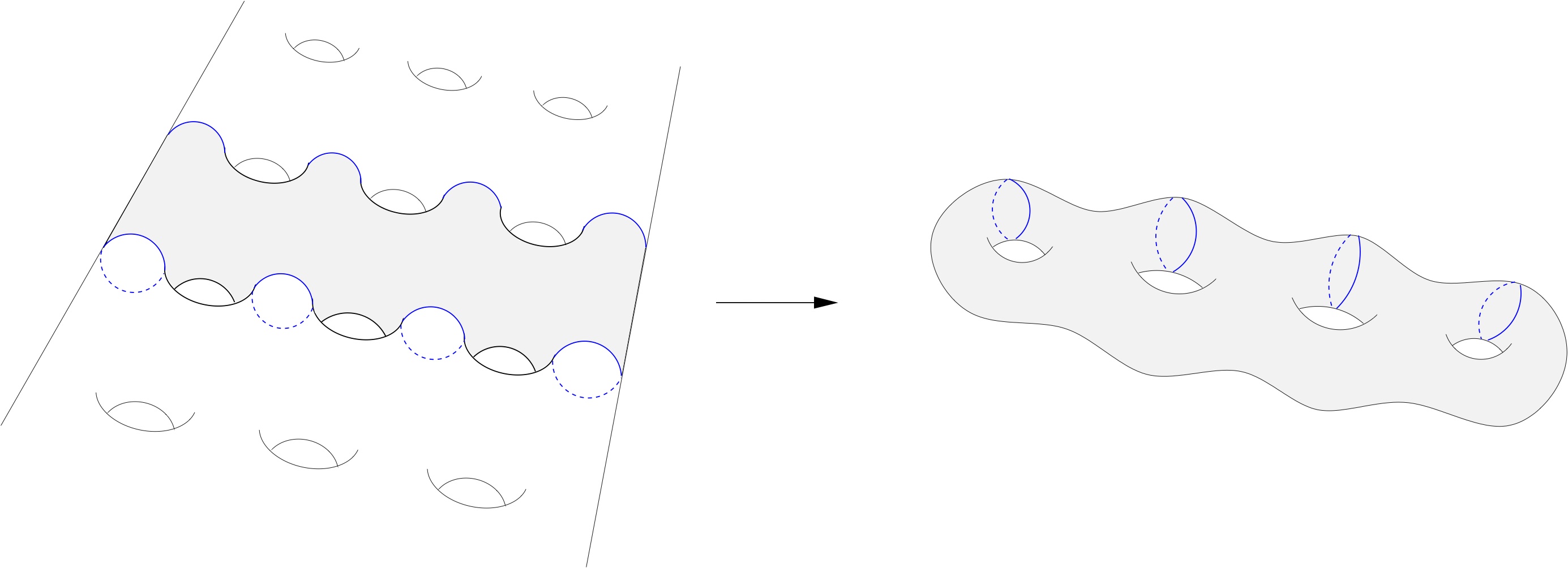
Figure 2: Construction of ladders

$\bullet$ Hyperbolic Flutes: these are, topologically, spheres with infinitely many punctures $e_{i}$ accumulating to one limit puncture $e$; the surface thus has one end for each puncture $e_{i}$ (called its finite ends), and an end corresponding to $e$, the infinite end of the flute. Geometrically, each end $e_{i}$ different from $e$ must be either a cusp (the quotient of a horoball $H_{\xi}$ of $\mathbf{H}^{2}$ by a parabolic subgroup $P_{\xi}$ fixing the center $\xi$ of $H_{\xi}$) or a funnel (the quotient of a half-plane of $\mathbf{H}^{2}$ by an infinite cyclic group of hyperbolic isometries).

We obtain workable models of flutes via infinitely generated Schottky groups. Define the attractive and repulsive domains $A(g,\tilde{o})$, $A(g^{-1},\tilde{o})$ of a parabolic or hyperbolic isometry $g$, with respect to some point $\tilde{o}\in\mathbf{H}^{2}$, respectively as

$$A(g^{\pm 1},\tilde{o})=\{x\in\mathbf{H}^{2}\;|\;d(x,\tilde{o})\geq d(x,g^{\pm 1}\tilde{o})\}$$

We say that $G$ is an infinitely generated Schottky group if it is generated by countable many hyperbolic isometries $S=(g_{n})$, in Schottky position with respect to some $\tilde{o}\in\mathbf{H}^{2}$, that is: $A(g_{n}^{\epsilon},\tilde{o})\cap A(g_{m}^{\epsilon^{\prime}},\tilde{o})=\emptyset\;\;\;\forall n,m\mbox{ and }\forall\epsilon,\epsilon^{\prime}\in\{\pm 1\}.$

By a ping-pong argument it follows that $G$ is discrete and free over the generating set $S$; moreover, its Dirichlet domain with respect to $\tilde{o}$ is

$$D(G,\tilde{o})=\mathbf{H}^{2}\setminus\bigcup_{g_{n}\in S}\left(A(g_{n},\tilde{o})\cup A(g_{n}^{-1},\tilde{o})\right)^{o}$$

If the axes of the hyperbolic generators do not intersect and the domains $A(g_{n}^{\pm 1},\tilde{o})$ accumulate to one boundary point $\zeta$ (or to different boundary points $E=\{\zeta_{k}\}$, all defining the same end of the quotient $X=G\backslash\mathbf{H}^{2}$) then the resulting surface $X=G\backslash\mathbf{H}^{2}$ is a hyperbolic flute: it has a cusp for every parabolic generator, a funnel for every hyperbolic generator, and an infinite end corresponding to $\zeta$ (or to the set $E$). For the construction of Schottky groups we will repeatedly make use of the following (cp. Appendix A.3 for a proof):

Lemma 39

Let $\tilde{o}\in\mathbf{H}^{2}$, and let $C,C^{\prime}$ two ultraparallel geodesics (i.e. with no common point in $\mathbf{H}^{2}\cup\partial\mathbf{H}^{2}$) such that $d(\tilde{o},C)=d(\tilde{o},C^{\prime})$. Then:

(i) there exists a unique hyperbolic isometry $g$ with axis perpendicular to $C,C^{\prime}$ and such that $g(C)=C^{\prime}$;

(ii) $g^{-1}\tilde{o}$ and $g\tilde{o}$ are obtained, respectively, by the hyperbolic reflections of $\tilde{o}$ with respect to $C,C^{\prime}$;

(iii) the Dirichlet domain $D(g,\tilde{o})$ has boundary $C\cup C^{\prime}$.

Example 40

The Asymmetric Hyperbolic Flute

We construct a hyperbolic flute $X=G\backslash\mathbf{H}^{2}$ with two rays $\alpha,\alpha^{\prime}$ having same origin such that:

(a) $\alpha^{\prime}\prec_{G}\alpha\not\prec_{G}\alpha^{\prime}$ (i.e. $\alpha^{\prime}\prec\alpha\not\prec\alpha^{\prime}$); therefore, $\alpha\not\approx_{G}\alpha^{\prime}$ and $B_{\alpha}\neq B_{\alpha^{\prime}}$;

(b) $d_{\infty}(\alpha,\alpha^{\prime})=\infty$.

We use the disk model for $\mathbf{H}^{2}$ with origin $\tilde{o}$. Let $\tilde{o}^{\prime}=-\frac{i}{10}$, and consider the geodesics $\widetilde{\alpha}=[\tilde{o},-i]$, $\widetilde{\alpha}^{\prime}=[\tilde{o},i]$. Then, let $R$ be the reflection with respect to the real axis, and consider the horoballs $H=H_{\tilde{\alpha}^{+}}(\tilde{o})$ and $H^{\prime}=H_{\tilde{\alpha}^{\prime+}}(\tilde{o}^{\prime})\supset R(H)$; finally, choose some positive sequence $\epsilon_{k}\searrow 0$.
Let $[\tilde{o},\zeta_{1}]$ be a ray making angle $\vartheta_{1}$ with $\widetilde{\alpha}$, let $\tilde{o}_{1}$ be the point on $[\tilde{o},\zeta_{1}]$ such that $d(\tilde{o}_{1},H)=\epsilon_{1}$, and let $C_{1}$ be the hyperbolic perpendicular bisector of the segment $[\tilde{o},\tilde{o}_{1}]$, with extremities $c_{1,+}$ and $c_{1,-}$, cp. Figure 3.a. Notice that, as $\epsilon_{1}>0$ the circle $C_{1}$ does not intersect $\widetilde{\alpha}$ (the extremity $c_{1,+}$ closest to $\tilde{\alpha}^{+}$ coincides with $\tilde{\alpha}^{+}$ if and only if $\tilde{o}_{1}\in\partial H$). Then, consider $R(C_{1})$ and rotate it clockwise around $\tilde{o}$ until it is tangent to $H^{\prime}$: call this new geodesic $C_{1}^{\prime}$ and its extremities $c_{1,+}^{\prime},c_{1,-}^{\prime}$.

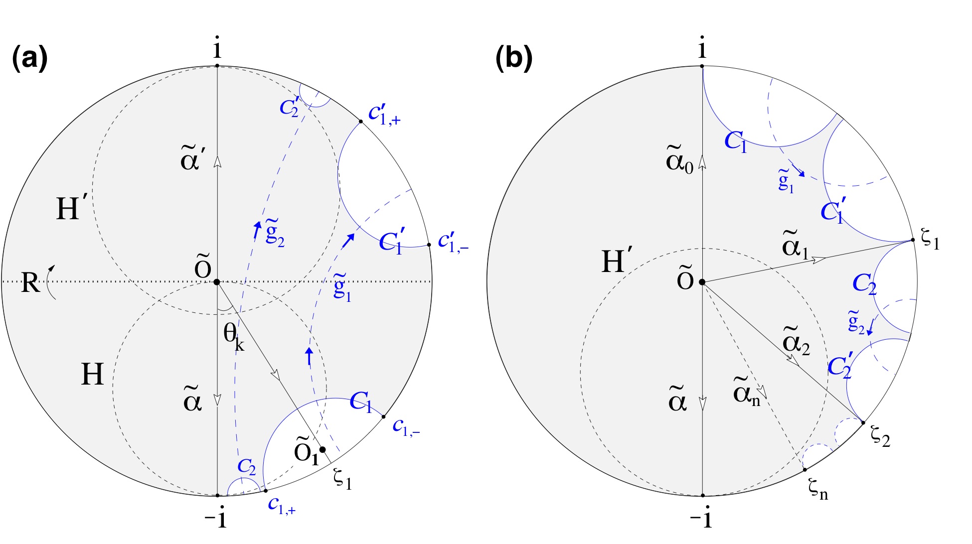
Figure 3: Asymmetric and Twisted Flutes

Let now $g_{1}$ be the hyperbolic isometry given by Lemma 39, with axis $\tilde{g}_{1}$ perpendicular to $C_{1},C^{\prime}_{1}$, and such that $g_{1}(C_{1})=C^{\prime}_{1}$ and $g_{1}^{-1}(\tilde{o})=\tilde{o}_{1}$. Then, construct $g_{2}$ analogously: that is, choose a ray $[\tilde{o},\zeta_{2}]$, for some $\zeta_{2}$ between $\widetilde{\alpha}^{+}$ and $c_{1,+}$, making angle $\vartheta_{2}<\vartheta_{1}$ with $\widetilde{\alpha}$; call $\tilde{o}_{2}$ the point on $[\tilde{o},\zeta_{2}]$ with $d(\tilde{o}_{2},H)=\epsilon_{2}$, and then let $C_{2}$, $C^{\prime}_{2}$, $\tilde{g}_{2}$ etc. as before. Repeating inductively this construction we obtain the infinitely generated group $G=<g_{1},g_{2},...,g_{k},...>$.

Moreover, choosing $\vartheta_{k+1}\ll\vartheta_{k}$, we can make the following conditions satisfied:

$$A(g_{n}^{\epsilon},\tilde{o})\cap A(g_{m}^{\tau},\tilde{o})=\emptyset\mbox{ for all }n\neq m\mbox{ and }\epsilon,\tau\in\{\pm 1\}$$ (12)

$$U_{n}(\widetilde{\alpha}\cup\widetilde{\alpha}^{\prime})\cap A(g_{n}^{\epsilon},\tilde{o})=\emptyset\mbox{ for all }n\in\mathbb{N}\mbox{ and }\epsilon\in\{\pm 1\}$$ (13)

where $U_{n}(\widetilde{\alpha}\cup\widetilde{\alpha}^{\prime})$ is the tubular neighbourhood of $\widetilde{\alpha}\cup\widetilde{\alpha}^{\prime}$ of width $n$.
Condition (12) says that $G$ is a discrete Schottky group. The quotient manifold $X=G\backslash\mathbf{H}^{2}$ is a hyperbolic flute, with infinite end corresponding to the set $E=\{\widetilde{\alpha}^{+},\widetilde{\alpha}^{\prime+}\}$. Let $\alpha$ and $\alpha^{\prime}$ be projections of $\widetilde{\alpha},\widetilde{\alpha}^{\prime}$ to $X$, with common origin $o$: they are rays, as their lifts stay in $D(G,\tilde{o})$ by construction.

Proof of Properties 40(a)&(b).

We have $\alpha\succ_{G}\alpha^{\prime}$ as $g_{n}\widetilde{\alpha}^{+}\rightarrow\widetilde{\alpha}^{\prime+}$ and $B_{\tilde{\alpha}}(\tilde{o},g_{n}^{-1}\tilde{o})\rightarrow 0$, by construction. On the other hand, for every sequence $h_{k}\in G$ such that $h_{k}\widetilde{\alpha}^{\prime+}\rightarrow\widetilde{\alpha}^{+}$, the points $h_{k}^{-1}\tilde{o}$ definitely lie in some of the attractive domains $A(g_{n},\tilde{o})$, which are exterior to $H^{\prime}$: thus, $B_{\tilde{\alpha}^{\prime}}(\tilde{o},h_{k}^{-1}\tilde{o})\!\geq\!\frac{1}{10}$ and does not tend to $0$. This proves that $\alpha\not\prec_{G}\alpha^{\prime}$. The other assertions in (a) follow from the construction of $G$ and Theorem 28. For (b), assume that $d_{\infty}(\alpha,\alpha^{\prime})<M$: then we could find arbitrarily large $t,t^{\prime}$ and $g_{t}\in G$ such that $d(\widetilde{\alpha}(t),g_{t}\widetilde{\alpha}^{\prime}(t^{\prime}))<M$. Let then $g_{n(t)}$ be the generator such that $g_{t}\widetilde{\alpha}^{\prime}\subset A(g_{n(t)}^{\epsilon},\tilde{o})$, for some $\epsilon\in\{\pm 1\}$. By (13) we deduce that $d(\widetilde{\alpha}(t),g_{t}\widetilde{\alpha}^{\prime}(t^{\prime}))\geq d(\widetilde{\alpha},A(g_{n(t)}^{\epsilon},\tilde{o}))\geq n(t)$ which shows that we necessarily have $n(t)=n$ for infinitely many, arbitrarily large $t$. Hence

$$\limsup_{t\rightarrow+\infty}d(\widetilde{\alpha}(t),g_{t}\widetilde{\alpha}^{\prime}(t^{\prime}))\geq\limsup_{t\rightarrow+\infty}d(\widetilde{\alpha}(t),A(g_{n}^{\epsilon},\tilde{o}))=\infty$$

a contradiction.$\Box$

Example 41

The Symmetric Hyperbolic Flute

We construct a hyperbolic flute $X=\widehat{G}\backslash\mathbf{H}^{2}$ with two rays $\alpha,\alpha^{\prime}$ having same origin such that:

(a) $\alpha\prec_{\widehat{G}}\succ\alpha^{\prime}$ (i.e. $\alpha\prec\succ\alpha^{\prime}$); therefore, $B_{\alpha}=B_{\alpha^{\prime}}$;

(b) $\alpha\not\approx_{G}\alpha^{\prime}$;

(c) $d_{\infty}(\alpha,\alpha^{\prime})=\infty$.

Let $G=<g_{1},...,g_{n},...>$ be the group constructed in the Example 40, and let $S$ be the symmetry with respect to $\tilde{o}$. Then, for every $n$, consider the hyperbolic translation $\hat{g}_{n}$ having axis $S[\tilde{g}_{n}]$ and attractive/repulsive domains $A(\hat{g}_{n}^{\pm 1},\tilde{o})=S[A(g_{n}^{\pm 1},\tilde{o})]$, and define $\hat{G}=<g_{1},\hat{g}_{1},...,g_{n},\hat{g}_{n},...>$.

Notice that, by symmetry, all these generators again satisfy the conditions (12) and (13), so $\hat{G}$ is a discrete Schottky group. Again, the quotient manifold $X=\hat{G}\backslash\mathbf{H}^{2}$ is a hyperbolic flute, with infinite end corresponding to the set $E=\{\widetilde{\alpha}^{+},\widetilde{\alpha}^{\prime+}\}$ and, with the same notations as above, the projections $\alpha$ and $\alpha^{\prime}$ on $X$ are rays.

Proof of Properties 41(a),(b)&(c).

We deduce as before that $\alpha\succ_{\hat{G}}\alpha^{\prime}$; but now we also have the sequence $\hat{g}_{n}$ such that $\hat{g}_{n}\widetilde{\alpha}^{\prime+}\rightarrow\widetilde{\alpha}^{+}$ and $B_{\alpha^{\prime}}(\tilde{o},\hat{g}_{n}^{-1}\tilde{o})\rightarrow 0$; so $\alpha^{\prime}\succ_{\hat{G}}\alpha$ too. As the rays $\alpha$ and $\alpha^{\prime}$ have a common origin, Theorem 28 implies that $B_{\alpha}=B_{\alpha^{\prime}}$. Again assertion (b) follows by construction, and (c) is proved as before.$\Box$

Example 42

The Twisted Hyperbolic Flute

We construct a hyperbolic flute $X=G\backslash\mathbf{H}^{2}$ with a family of rays $\alpha_{n}$ having same origin and converging to a ray $\alpha$ such that:

(a) $\;\alpha_{n}\approx_{G}\alpha_{m}$ $\forall n,m$; therefore, $d_{\infty}(\alpha_{n},\alpha_{m})<\infty$ and $B_{\alpha_{n}}=B_{\alpha_{m}}$ $\forall n,m$;

(b) $\;d_{\infty}(\alpha_{n},\alpha)=\infty$ $\forall n$;

(c) $B_{\alpha_{0}}=\lim_{n\rightarrow+\infty}B_{\alpha_{n}}\neq B_{\alpha}$.

Again, in the disk model for $\mathbf{H}^{2}$ with origin $\tilde{o}$, consider a sequence of boundary points $\zeta_{0}=i$, $\zeta_{n}=e^{i\vartheta_{n}}$, for a decreasing sequence $\frac{\pi}{2}\geq\vartheta_{n}\searrow-\frac{\pi}{2}$. Then, for every $n\geq 1$ choose a pair of ultraparallel geodesics $C_{n},C^{\prime}_{n}$ such that $d(\tilde{o},C_{n})=d(\tilde{o},C^{\prime}_{n})=d_{n}$, each cointained in the disk sector $[\zeta_{n-1},\tilde{o},\zeta_{n}]$, and with points at infinity respectively equal to $\zeta_{n-1}$, $\zeta_{n}$. Finally, let $g_{n}$ be the hyperbolic isometry with $g_{n}(C_{n})=C^{\prime}_{n}$ whose axis is perpendicular to $C_{n},C^{\prime}_{n}$, given by Lemma 39, cp. Figure 3.b, and set $\widetilde{\alpha}_{n}=[\tilde{o},\zeta_{n}]$, $\widetilde{\alpha}=[\tilde{o},-i]$.
Moreover, if $H^{\prime}=H_{\tilde{\alpha}^{+}}(\tilde{o}^{\prime})$ for $\tilde{o}^{\prime}=\frac{i}{10}$, we can choose the $d_{n}\gg 0$ in order that the following condition is satisfied:

$$H^{\prime}\cap A(g_{n}^{\pm 1},\tilde{o})=\emptyset\mbox{ for all }n$$ (14)

Define $G$ as the group generated by all the $g_{n}$. Again, $G$ is an infinitely generated Schottky group, and the quotient manifold $X=G\backslash\mathbf{H}^{2}$ is a flute whose infinite end corresponds to the set $E=\{\widetilde{\alpha}^{+},\widetilde{\alpha}_{n}^{+}\;|\;n\geq 0\}$. The projections $\alpha_{n}$ and $\alpha$ of all the $\widetilde{\alpha}_{n},\widetilde{\alpha}$ on $X$ are rays, by construction, such that $\alpha_{n}\rightarrow\alpha$.

Proof of Properties 42(a),(b)&(c).

The rays $\alpha_{n}$ are all $G$-equivalent by construction, as $\widetilde{\alpha}_{n}^{+}=g_{n}\widetilde{\alpha}_{n-1}^{+}$ for all $n$. The other assertions in (a) follow from the discussion after Definition 27(actually, as we are in strictly negative curvature, we have $d_{\infty}(\alpha_{n},\alpha_{m})=0$).On the other hand, by (14), all the images by $G$ of $\widetilde{\alpha}_{n}$ are exterior to the horoball $H^{\prime}$, exceptly for $\widetilde{\alpha}_{n}$ itself; thus if $s\gg 0$ we have $d(g\widetilde{\alpha}_{n},\widetilde{\alpha}(s))\!>\!s$ for all $g$. It follows that $d_{\infty}(\alpha_{n},\alpha)\geq\frac{1}{2}\limsup_{s\rightarrow+\infty}\inf_{g\in G}d(g\widetilde{\alpha}_{n},\widetilde{\alpha}(s))=+\infty$. To conclude we have to prove that $B_{\alpha_{0}}\neq B_{\alpha}$, and by Theorem 28 it is enough to show that $\alpha\not\succ_{G}\alpha_{0}$. But for any sequence $h_{n}$ with $h_{n}\widetilde{\alpha}^{+}\rightarrow\widetilde{\alpha}_{0}^{+}$ we have $B_{\tilde{\alpha}}(\tilde{o},h_{n}\tilde{o})<-\frac{1}{10}$, since by construction this is true for all nontrivial $g$ in $G$.$\Box$

Remark 43

The discontinuity (c) can be interpreted geometrically as follows.
Consider the maximal horoballs $H_{\tilde{\alpha}^{+}}^{max}(o^{\prime}),H_{\tilde{\alpha}_{n}^{+}}^{max}(o^{\prime})$, for the projection $o^{\prime}$ of $\tilde{o}^{\prime}$. It is easy to see that $H_{\tilde{\alpha}^{+}}^{max}(o^{\prime})=H_{\tilde{\alpha}^{+}}(\tilde{o}^{\prime})$, as all the $g\tilde{o}^{\prime}$, for $g\neq 1$, stay far away from $H^{\prime}$, by construction. Moreover, since $o^{\prime}\in\alpha_{0}$ and $\alpha_{0}$ is a ray, we also deduce that $H_{\tilde{\alpha}_{0}^{+}}^{max}(o^{\prime})=H_{\tilde{\alpha}_{0}^{+}}(\tilde{o}^{\prime})$ precisely. Now $B_{\alpha_{n}}(o,o^{\prime})=B_{\alpha_{0}}(o,o^{\prime})$, so formula (5) shows that $d(\tilde{o},H^{max}_{\tilde{\alpha}_{n}^{+}}(o^{\prime}))=d(\tilde{o},H^{max}_{\tilde{\alpha}_{0}^{+}}(o^{\prime}))$; then, by rotational symmetry, $H_{\tilde{\alpha}_{n}^{+}}^{max}(o^{\prime})$ is the horoball centred at $\tilde{\alpha}_{n}^{+}$ having the same Euclidean radius as $H_{\tilde{\alpha}_{0}^{+}}(\tilde{o}^{\prime})$. Therefore the discontinuity can be read in terms of a discontinuity in the limit of the maximal horoballs: in fact, the $H_{\tilde{\alpha}_{n}}^{max}(o^{\prime})$’s converge for $n\rightarrow\infty$ to $H_{\tilde{\alpha}^{+}}(-\tilde{o}^{\prime})$, which is strictly smaller than the maximal horoball $H_{\tilde{\alpha}^{+}}(\tilde{o}^{\prime})$ of the limit ray.

Example 44

The Hyperbolic Ladder

We construct a hyperbolic ladder which is a Galois covering $X\rightarrow\Sigma_{2}$ of a hyperbolic surface of genus $2$, with automorphisms group $\Gamma\cong\mathbb{Z}$, such that:

(a) $X$ has distance-asymptotic rays $\alpha,\alpha^{\prime}$ with $\alpha\prec\succ\alpha^{\prime}$, but $B_{\alpha}\neq B_{\alpha^{\prime}}$;

(b) ${\cal B}X$ consists of 4 points;

(c) $\partial X$ consists of a continuum of points;

(d) the limit set $L\Gamma=\overline{\Gamma x_{0}}\cap\partial X$ depends on the choice of the base point $x_{0}$, and for some $x_{0}$ it is included in $\partial X-{\cal B}X$.

We construct $X$ by glueing infinitely many pairs of hyperbolic pants.
The following properties of hyperbolic pants are well-known:

Lemma 45 ([16], [40])

Let $H^{+},H^{-}$ be two identical right-angled hyperbolic hexagons with alternating edges labelled respectively by $a^{\pm},b^{\pm},c^{\pm}$ and opposite edges $\alpha^{\pm},\beta^{\pm},\gamma^{\pm}$. Let $P$ the hyperbolic pant obtained by glueing them along $a^{\pm},b^{\pm},c^{\pm}$; the identified edges $a,b,c$ are called the seams of $P$, and the resulting boundaries $\alpha=\alpha^{+}\cup\alpha^{-},\beta=\beta^{+}\cup\beta^{-},\gamma=\gamma^{+}\cup\gamma^{-}$ of $P$ are closed geodesics called the cuffs. The seams are the shortest geodesic segments connecting the cuffs of $P$ and, reciprocally, the cuffs are the shortest ones connecting the seams.

Now, we start from infinitely many copies $P_{n}$, $P^{\prime}_{n}$, for $n\in\mathbb{Z}$, of the same pair of pants $P$, and we assume that $\ell(b)=\ell(c)=L>\ell=\ell(a)$. We glue them as in figure 4, by identifying via the identity the cuffs $\alpha_{n}$ with $\alpha^{\prime}_{n}$, and the cuffs $\beta_{n}$, $\beta^{\prime}_{n}$ with $\gamma_{n-1}$, $\gamma^{\prime}_{n-1}$ respectively (with no twist), obtaining a complete hyperbolic surface $X=N\backslash\mathbf{H}^{2}$. Remark that, if $\Sigma_{2}=G\backslash\mathbf{H}^{2}$ is the hyperbolic surface obtained from $P_{0}\cup P^{\prime}_{0}$ by identifying $\alpha_{0}$ to $\alpha^{\prime}_{0}$ and $\beta_{0}$, $\beta^{\prime}_{0}$ respectively to $\gamma_{0}$, $\gamma_{0}^{\prime}$, there is a natural covering projection $X\rightarrow\Sigma_{2}$, with automorphism group $\Gamma\cong\mathbb{Z}\cong G/N$. The group $\Gamma$ acts on $X$ by “translations” $T_{k}$, sending $P_{n}\cup P^{\prime}_{n}$ into $P_{n+k}\cup P^{\prime}_{n+k}$.

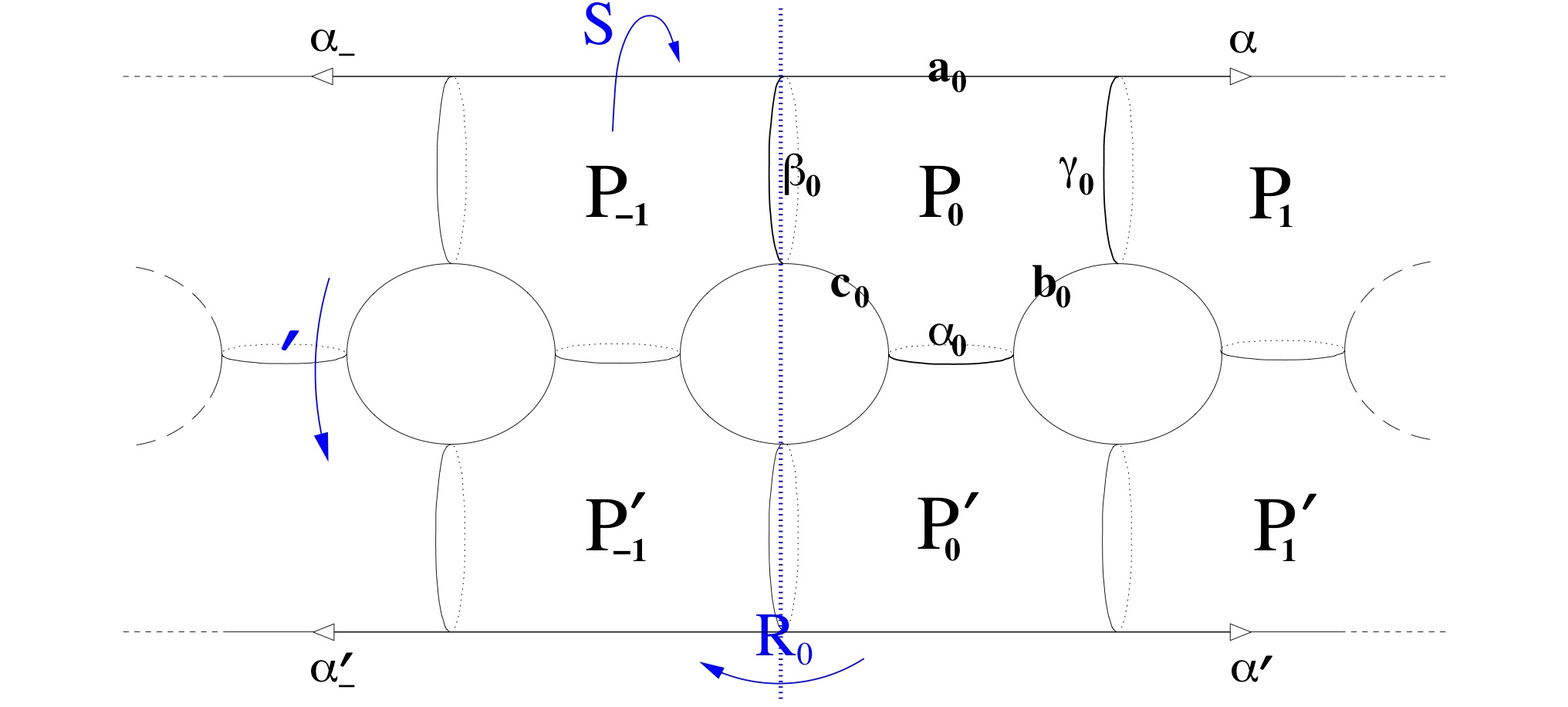
Figure 4: The Hyperbolic Ladder

We define $\alpha\!=\!\bigcup_{k\geq 0}a_{k}$, $\alpha_{-}\!=\!\bigcup_{k<0}a_{k}$, $\alpha^{\prime}\!=\!\bigcup_{k\geq 0}a^{\prime}_{k}$, $\alpha^{\prime}_{-}\!=\!\bigcup_{k<0}a^{\prime}_{k}$ and set $\mathcal{A}=\alpha\cup\alpha_{-}$, $\mathcal{A}^{\prime}=\alpha^{\prime}\cup\alpha^{\prime}_{-}$. Notice that the surface $X$ is also endowed of:

– a natural flip symmetry, denoted ^′, obtained by sending a point in $P_{k}$ to the corresponding point in $P^{\prime}_{k}$; let $\mathcal{F}=Fix(^{\prime})$ and call the top and the bottom of $X$ the (closure of) the two connected components of $X-\mathcal{F}$ interchanged by ^′;

– a natural mirror symmetry $S$, obtained interchanging each point on a pant $P_{k}$ (resp. $P^{\prime}_{k}$) with the corresponding point lying on the same pant, but on the opposite hexagon; if $\mathcal{M}=\bigcup_{k\in\mathbb{Z}}b_{k}\cup b^{\prime}_{k}\cup c_{k}\cup c^{\prime}_{k}$, we have $Fix(S)=\mathcal{A}\cup\mathcal{A}^{\prime}\cup\mathcal{M}$, and we will call the back and the front of $X$ the closure of the two connected components of $X-Fix(S)$ interchanged by $S$;

– a group of reflections $R_{n}$ with respect to $\beta_{n}\cup\beta^{\prime}_{n}$, exchanging $P_{n+k}\cup P^{\prime}_{n+k}$ with $P_{n-k-1}\cup P^{\prime}_{n+k-1}$.

Lemma 46

(i) Every minimizing geodesic does not cross twice neither $\mathcal{A}$, $\mathcal{A}^{\prime}$, $\mathcal{F}$ nor $\mathcal{M}$;

(ii) every quasi-ray is strongly asymptotic to one of the four rays $\alpha,\alpha_{-},\alpha^{\prime},\alpha^{\prime}_{-}$.

Proof.

(i) Assume that $\gamma$ is a minimizing geodesic between $x$ and $y$, crossing $\mathcal{A}$ twice, at two points $x_{1},y_{1}$. Break it as $\gamma=\gamma_{1}\cup[x_{1},y_{1}]\cup\gamma_{2}$, where $[x_{1},y_{1}]$ is the subsegment between $x_{1}$ and $y_{1}$. Then, using the mirror symmetry $S$, we would obtain a curve $\hat{\gamma}=\gamma_{1}\cup S[x_{1},y_{1}]\cup\gamma_{2}$ of same length, still connecting $x$ to $y$, but singular at $x_{1}$ and $y_{1}$; hence, it could be shortened, which is a contradiction. The proof is the same for $\mathcal{A}^{\prime},\mathcal{B}$, and using the flip simmetry ^′ one analogusly proves that a minimizing geodesic cannot cross twice $\mathcal{F}$.
For (ii), let us first show that, if $\gamma$ is a quasi-ray included, say, in the top-front of $X$, then either $d_{\infty}(\gamma,\alpha)=0$ or $d_{\infty}(\gamma,\alpha_{-})=0$. Actually, assume that $p_{n}=\gamma(t_{n})$ is a sequence such that $d(p_{n},\mathcal{A})>\epsilon$, for $n\geq 0$ and $t_{n}\rightarrow\infty$. Consider the projections $q_{n}$ of $p_{n}$ on $\mathcal{A}$, which we may assume at distance $d(q_{n},q_{n+1})\gg 0$; as $\gamma$ is included in a simply connected open set of $X$ containing the bi-infinite geodesic $\mathcal{A}$, we can use hyperbolic trigonometry (cp. Lemma 49 in the §A.3) to deduce that $\ell(\gamma|_{[t_{n},t_{n+1}]})\geq q_{n}q_{n+1}+\delta(\epsilon)$, for a universal function $\delta(\epsilon)>0$.
As $p_{0}p_{n}\leq q_{0}q_{n}+2\mbox{diam}(P)$, we obtain

$$\Delta(\gamma|_{[t_{0},t_{N}]})\geq\sum_{n=0}^{N-1}q_{n}q_{n+1}+N\delta(\epsilon)-q_{0}q_{N}-2\mbox{diam}(P)=N\delta(\epsilon)-2\mbox{diam}(P)$$

which diverges as $N\rightarrow\infty$; so, $\Delta(\gamma)$ is not bounded, a contradiction. As $\epsilon$ is arbitrary, this shows that $\gamma$ is strongly asymptotic either to $\alpha$ or to $\alpha_{-}$. Finally, if $\gamma$ is a quasi-ray which is not included in the top-front of $X$, we can use the symmetries $S$ and ^′ to define, from $\gamma$, a curve $\hat{\gamma}$ fully included in the top-front of $X$, by reflecting the subsegments which do not lie in the top-front of $X$. This new curve still has bounded excess (as it has the same lenght as $\gamma$ on every interval, and the distance between endpoints reduces at most of $2\mbox{diam}(P)$) so, as we just proved, it is strongly asymptotic either to $\alpha$ or to $\alpha_{-}$. In particular, $\hat{\gamma}$ finally does not intersect $C$; so, $\gamma|_{[t_{0},+\infty]}$, for some $t_{0}\gg 0$, is included in an $\epsilon$-neighborhood of $\mathcal{A}$, for arbitrary $\epsilon$, and therefore it is strongly asymptotic to one of the four rays $\alpha,\alpha_{-},\alpha^{\prime},\alpha^{\prime}_{-}$.$\Box$

Proof of 44(a),(b),(c)&(d) of Example 44.

(a) The geodesic segments $a_{n}$ are the shortest curves connecting the cuffs $\beta_{n},\gamma_{n}$ of $P_{n}$: this implies that $\alpha$ cannot be shortened, so it is a ray; similarly for $\alpha^{\prime}$. Let now $x_{0}=a_{0}\cap\beta_{0}$, $x_{n}=T_{n}(x_{0})$ and let $x^{\prime}_{n}$ be their flips; finally, consider a sequence of minimizing segments $\eta_{n}=[x_{0},x^{\prime}_{2n}]$ and their inverse paths $-\eta_{n}$. By (i) above, we know that $\eta_{n}$ is included in the front (or the back) of $X$; moreover, it can be broken as $\eta_{n}=\eta^{t}_{n}\cup\eta^{b}_{n}$ where $\eta^{t}_{n},\eta^{b}_{n}$ respectively are subsegments in the top and in the bottom of $X$ meeting at some $p_{n}\in\mathcal{F}$ . Therefore, each of these segments stays in a simply connected open set of $X$, isometric to an open set of $\mathbf{H}^{2}$; then, since $d(p_{n},\alpha)=d(p_{n},\alpha^{\prime})<\mbox{diam}(P)$ we can apply standard hyperbolic trigonometry to deduce that $\eta_{n}$ makes an angle $\vartheta_{n}$, with either $\alpha$ or $\alpha^{\prime}$, such that

$$\tan\vartheta_{n}\leq\frac{\tanh(diam(P))}{\sinh(n\ell)}\rightarrow 0,\;\mbox{ for }n\rightarrow\infty.$$

By possibly replacing $\eta_{n}$ with $R_{n}(-\eta_{n})^{\prime}$, we find a sequence of minimizing segments $[x_{0},x^{\prime}_{2n}]\rightarrow\alpha$, hence $\alpha^{\prime}\succ\alpha$. The converse relation $\alpha\succ\alpha^{\prime}$ is analogous. Let us now show that $B_{\alpha}\neq B_{\alpha^{\prime}}$. It is enough to show that $B_{\alpha}(x_{0},x^{\prime}_{0})>0$; then clearly, by the flip symmetry, we will deduce $B_{\alpha^{\prime}}(x_{0},x^{\prime}_{0})=B_{\alpha}(x^{\prime}_{0},x_{0})<0$. Let us compute $B_{\alpha}(x_{0},x_{0}^{\prime})=\lim_{n\rightarrow\infty}x_{0}x_{n}-x_{n}x_{0}^{\prime}$. Let $\nu_{n}=[x_{n},x_{0}^{\prime}]$ be a minimizing segment intersecting $\mathcal{F}$ at some $p\in\hat{\alpha}_{k}$, and break it as $\nu_{n}=\nu^{t}_{n}\cup\hat{\nu}_{n}\cup\nu^{b}_{n}$ where $\hat{\nu}_{n}$ is the maximal subsegment of $\nu_{n}$ included in $P_{k}\cup P^{\prime}_{k}$; then,

$$x_{n}x_{0}^{\prime}\geq\ell(\nu^{t}_{n})+d(\gamma_{k},\beta^{\prime}_{k})+\ell(\nu^{b}_{n})\geq(n-1)\ell+2L\geq(n+1)\ell$$

while clearly $x_{0}x_{n}=n\ell$; so, $B_{\alpha}(x_{0},x_{0}^{\prime})\geq\ell$.

(b) One proves analogously that $\alpha_{-}$ and $\alpha^{\prime}_{-}$ are rays defining different Busemann functions, while it is clear that $B_{\alpha}$ and $B_{\alpha^{\prime}}$ are different from $B_{\alpha_{-}},B_{\alpha^{\prime}_{-}}$. Therefore ${\cal B}X$ has at least 4 points. On the other hand, by Proposition 46(ii), every quasi-ray in $X$ is strongly asymptotic to one of the four above, thus defining the same Busemann function. This shows that ${\cal B}X$ has precisely four points.

(c)-(d) Clearly, the orbits $\Gamma x_{0}$ and $\Gamma x^{\prime}_{0}$ accumulate to $B_{\alpha}$ and $B_{\alpha^{\prime}}$. Let now $x(t)$ be a continuous curve from $x_{0}=x(0)$ to $x^{\prime}_{0}=x(1)$, and set $x_{n}(t)=T_{n}(x(t))$. For any fixed $t$, let $B_{(x_{n})(t)}$ be the limit of (a subsequence of) $x_{n}(t)$, for $n\rightarrow\infty$. The family $B_{(x_{n})(t)}$ defines a continuous curve in $\partial X$ connecting $B_{\alpha}$ to $B_{\alpha^{\prime}}$, as $\|B_{(x_{n})(t)}-B_{(x_{n})(s)}\|_{\infty}\leq 2d(x_{n}(t),x_{n}(s))$; since it is non-constant, its image is an uncountable subset of $\partial X$. It remains to exhibit an orbit accumulating to a point of $\partial X\setminus{\cal B}X$. Let $y_{0}\in\alpha_{0}$: we affirm that $y_{n}=T_{n}y_{0}$ is such an orbit. Actually, if $y_{n}$ converged to one of the four Busemann functions, say $B_{\alpha}$, then we would also have $y_{n}=y^{\prime}_{n}\rightarrow B_{\alpha^{\prime}}$, as the flip symmetry preserves the orbit and exchanges $\alpha$ with $\alpha^{\prime}$. Hence we would get $B_{\alpha}=B_{\alpha^{\prime}}$, a contradiction.$\Box$

Remark 47

The surface $X$ is quasi-isometric to $\mathbb{Z}$, hence it is a Gromov-hyperbolic metric space. Its boundary as a Gromov-hyperbolic space $X^{g}(\infty)$ (cp. [10], [34]) consists of two points. So, the Busemann boundary and the horoboundary prove to be finer invariants than $X^{g}(\infty)$ (as they are not defined up to bounded functions, so they are not invariant by quasi-isometries).

Appendix A Appendix

A.1 Rays on Riemannian manifolds.

Lemma 48

Let $\beta$ be a quasi-ray and $x,y\in X$ such that $B_{\beta}(x,y)\!=\!d(x,y).\!$ Then:

(i) $x$ and $y$ minimize the distance between the horospheres $H_{\beta^{+}}(x)$ and $H_{\beta^{+}}(y)$;

(ii) $y$ is the only projection to $H_{\beta^{+}}(y)$ of every $z\!\in\![x,y]$, exceptly possibly for $x$.

Proposition 14 For any quasi-ray $\beta$ we have: $\;B_{\beta}(x,y)=d(x,y)\;\Leftrightarrow\;\overrightarrow{xy}\prec\beta$. In particular, if $B_{\beta}(x,y)=d(x,y)$, the extension of any minimizing segment $[x,y]$ beyond $y$ is always a ray.

Theorem 16   Assume that $\alpha,\beta$ are rays in $X$ with origins $a,b$ respectively. The following conditions are equivalent:

(a) $B_{\alpha}(x,y)\!=\!B_{\beta}(x,y)$ $\forall x,y\in X$;

(b) $\alpha\prec\succ\beta$ and $B_{\alpha}(a,b)=B_{\beta}(a,b)$;

(c) $\alpha$ and $\beta$ are visually equivalent from every $o\in X$.

Proof of Lemma 48. (i) follows from the fact that any two points $x^{\prime},y^{\prime}$ respectively in $H_{\beta^{+}}(x),H_{\beta^{+}}(y)$ satisfy $d(x^{\prime},y^{\prime})\geq B_{\beta}(x^{\prime},y^{\prime})=B_{\beta}(x,y)=d(x,y)$. In particular, $y$ is a projection to $H_{\beta^{+}}(y)$ of any point $z\in[x,y]$, as

$$xz+zy=xy=d(x,H_{\beta^{+}}(y))\leq xz+d(z,H_{\beta^{+}}(y)).$$

Moreover, let $z\in[x,y]$, $z\neq x$, and assume that $q$ is a projection of $z$ on $H_{\beta}(y)$ different from $y$. Then, the angle between $[x,z]$ and $[z,q]$ would be different from $\pi$; hence $xq<xz+zq$ and

$$d(x,H_{\beta^{+}}(y))<xz+zq=xz+zy=d(x,H_{\beta^{+}}(y))$$

a contradiction.$\Box$

Proof of Proposition 14. Let $\alpha\!=\!\overrightarrow{xy}$, with $x\!=\!\alpha(0)$, $y\!=\!\alpha(\overline{s})$. Assume $\alpha\!\prec\!\beta$. So, there exist minimizing geodesic segments $\alpha_{n}=[a_{n},b_{n}]\rightarrow\alpha$ such that $a_{n}\!=\!\alpha_{n}(0)\rightarrow x$, $b_{n}\!=\!\alpha_{n}(s_{n})\!=\!\beta(t_{n})\rightarrow\beta^{+}$, for sequences $s_{n},t_{n}\rightarrow+\infty$. Let $s$ be fixed and $\epsilon$ arbitrary. There exists $N(s,\epsilon)$ such that $d(\alpha_{n}(s),\alpha(s))<\epsilon$ and $d(a_{n},x)<\epsilon$ for $n>N(s,\epsilon)$; therefore

$$B_{\beta}(x,\alpha(s))=\lim_{n\rightarrow\infty}xb_{n}-b_{n}\alpha(s)\eqsim_{\epsilon}\lim_{n\rightarrow\infty}xb_{n}-b_{n}\alpha_{n}(s)=s$$

and as $\epsilon$ is arbitrary, this shows that $B_{\beta}(x,\alpha(s))=s=d(x,\alpha(s))$ for all $s$, hence $B_{\beta}(x,y)=d(x,y)$. Conversely, assume that $B_{\beta}(x,y)=d(x,y)$. Then:

$$s=\overline{s}-(\overline{s}-s)\leq B_{\beta}(x,y)-B_{\beta}(\alpha(s),y)=B_{\beta}(x,\alpha(s))\leq s\;\;\;\forall s\in[0,\overline{s}]$$

and we deduce that $B_{\beta}(x,x^{\prime})=d(x,x^{\prime})$ for all $x,x^{\prime}$ on $\alpha$ between $x$ and $y$. Now, fix $0<\epsilon<\overline{s}$ and consider minimizing geodesic segments $\alpha^{\epsilon}_{n}=[\alpha(\epsilon),\beta(n)]$; up to a subsequence, they converge, for $n\rightarrow\infty$, to a ray $\alpha^{\epsilon}$ which is, by definition, a coray of $\beta$. So (as we previously proved)

$$B_{\beta}(\alpha(\epsilon),\alpha^{\epsilon}(s))=B_{\alpha^{\epsilon}}(\alpha(\epsilon),\alpha^{\epsilon}(s))=s\;\;\;\forall s>0$$

But then, for $s>\epsilon$, $\alpha(s)$ and $\alpha^{\epsilon}(s-\epsilon)$ are both projections of $\alpha(\epsilon)$ to the horosphere $H_{\beta^{+}}(\alpha(s))$ and, by Lemma 48(ii), we know that they coincide. This shows that $\alpha^{\epsilon}=\alpha|_{\epsilon,+\infty}$ and that $\alpha^{\epsilon\,\prime}_{n}(0)$ tend to $\alpha^{\prime}(\epsilon)$, for every fixed $\epsilon>0$; by a diagonal argument we then build a sequence of minimizing geodesic segments $\alpha_{k}=\alpha^{\epsilon_{k}}_{n_{k}}$, for $\epsilon_{k}\rightarrow 0$ and $n_{k}\rightarrow+\infty$, such that $\alpha_{k}\rightarrow\alpha$. Thus $\alpha\prec\beta$.$\Box$

Proof of Theorem 16.
Let us show that (a) $\Rightarrow$ (b). Assume that $B_{\alpha}=B_{\beta}$, and let $b=\beta(0),y=\beta(t)$. As $B_{\alpha}(b,y)=B_{\beta}(b,y)=d(b,y)$, we deduce by Proposition 14 that $\beta\prec\alpha$. One proves that $\alpha\prec\beta$ analogously.

Conversely, let us show that (b) $\Rightarrow$ (a). Assume that $\alpha\prec\beta$, so we have geodesic segments $\alpha_{n}=[a_{n},b_{n}]\rightarrow\alpha$ with $a_{n}=\alpha_{n}(0)\rightarrow a$, $b_{n}=\beta(t_{n})=\alpha_{n}(s_{n})\rightarrow\beta^{+}$; moreover, let as before $N(s,\epsilon)$ such that $d(\alpha_{n}(s),\alpha(s))<\epsilon$ for $n>N(s,\epsilon)$. Then, for every $x$ and $n>N(s,\epsilon)$:

$$a\alpha(s)-\alpha(s)x\;\eqsim_{\epsilon}\;s-\alpha_{n}(s)x\;\leq\;s-\left(b_{n}x-b_{n}\alpha_{n}(s)\right)$$

and, as $b_{n}\alpha_{n}(s)=s_{n}-s$ we deduce that

$$a\alpha(s)-\alpha(s)x\;\apprle_{\epsilon}\;s_{n}-b_{n}x\;=\;(s_{n}\!-\!t_{n})+(t_{n}\!-b_{n}x)\;\leq\;B_{\beta}(a_{n},b)+B_{\beta}(b,x)$$

by monotonicity of the Busemann cocycle. Taking limits for $s\rightarrow\infty$ we deduce that $B_{\alpha}(a,x)\apprle_{\epsilon}B_{\beta}(a,x)$ for all $x$ and, as $\epsilon$ is arbitrary, $B_{\alpha}(a,x)\leq B_{\beta}(a,x)$. From $\beta\prec\alpha$ we deduce analogously that $B_{\beta}(b,x)\leq B_{\alpha}(b,x)$. Therefore:

$$B_{\beta}(b,x)\leq B_{\alpha}(b,x)=B_{\alpha}(b,a)+B_{\alpha}(a,x)\leq B_{\alpha}(b,a)+B_{\beta}(a,b)+B_{\beta}(b,x)$$

and since $B_{\alpha}(b,a)=B_{\beta}(b,a)$ we get the conclusion.

Let us now prove that (a) $\Rightarrow$ (c). Assume again that $B_{\alpha}=B_{\beta}$, and let $o\in X$. Let $\gamma$ be a limit of (a subsequence of) geodesic segments $\gamma_{n}=[o,\alpha(n)]$; then $\gamma$ is a ray (by the Properties 9) and, by definition, is a coray to $\alpha$. Then, by Proposition 14

$$B_{\beta}(o,\gamma(t))=B_{\alpha}(o,\gamma(t))=d(o,\gamma(t))$$

which, by the same Proposition, also implies that $\gamma\prec\beta$.
Finally, let us show that (c) $\Rightarrow$ (a). The functions $B_{\alpha}(a,\cdot)$ and $B_{\beta}(b,\cdot)$ are Lipschitz, hence differentiable almost everywhere. Let $o$ be a point of differentiability for both $B_{\alpha}(a,\cdot)$ and $B_{\beta}(b,\cdot)$, and let $\gamma$ be a ray from $o$ which is a coray to $\alpha$ and $\beta$. Then $B_{\alpha}(o,\gamma(t))=d(o,\gamma(t))=B_{\beta}(o,\gamma(t))$ for all $t$, which implies that $grad_{o}B_{\alpha}(a,\cdot)=\gamma^{\prime}(0)=grad_{o}B_{\beta}(b,\cdot)$. So $B_{\alpha}(a,\cdot)$ and $B_{\beta}(b,\cdot)$ are Lipschitz functions whose gradient is equal almost everywhere, hence they differ by a constant and $B_{\alpha}=B_{\beta}$.$\Box$

A.2 Rays on Hadamard spaces.

Proposition 18 Let $\widetilde{X}$ be a Hadamard space:

(i) if $\alpha,\beta$ are rays, then $d_{\infty}(\alpha,\beta)<\infty\;\Leftrightarrow\;B_{\alpha}=B_{\beta}\;\;\Leftrightarrow\;\alpha\prec\beta$.

Moreover, two rays with the same origin are Busemann equivalent iff they coincide, so the restriction of the Busemann map $B_{o}\!:\!{\cal R}_{o}(\widetilde{X})\rightarrow\partial\widetilde{X}$ is injective;

(ii) for any $o\in\tilde{X}$, the restriction of the Busemann map $B_{o}:{\cal R}_{o}(\widetilde{X})\rightarrow\partial\widetilde{X}$ is surjective, hence ${\cal B}\tilde{X}={\cal B}_{o}\tilde{X}=\partial\tilde{X}$;

(iii) the Busemann map $B$ is continuous.

Uniform Approximation Lemma 19 Let $\widetilde{X}$ be a Hadamard space.
For any compact set $K$ and $\epsilon>0$, there exists a function $T(K,\epsilon)$ such that for any $x,y\in K$ and any ray $\alpha$ issuing from $K$, we have $|B_{\alpha}(x,y)-b_{\alpha(t)}(x,y)|\leq\epsilon$, provided that $t\geq T(K,\epsilon)$.

Proof of Lemma 19.

First notice that, by the cocycle condition (holding for $b_{\alpha(t)}$ as well as for $B_{\alpha}$ we can assume that $x=\alpha(0)=a$. Then, let $z=\alpha(t)$, $z^{\prime}=\alpha(t^{\prime})$ for $t^{\prime}>t$, and let us estimate $b_{z^{\prime}}(a,y)-b_{z}(a,y)=(yz+zz^{\prime})-yz^{\prime}$. Assume that $K\subset B(a,r)$, denote by $y^{\prime}$ the projection of $y$ on $\alpha$ and consider $\vartheta=\widehat{yza}$. The right triangle $[y,y^{\prime},z]$ has catheti $yy^{\prime}\leq r$ and $zy^{\prime}\geq t-r$ (as $ay^{\prime}\leq r$); by comparison with a Euclidean triangle, we deduce that $0<\vartheta\leq\vartheta_{0}<\pi$ with $\tan\vartheta_{0}=r/(t-r)$. Comparing now the triangle $[y,z,z^{\prime}]$ with an Euclidean triangle $[y_{0},z_{0},z_{0}^{\prime}]$ such that $\widehat{y_{0}z_{0}z^{\prime}_{0}}=\pi-\vartheta_{0}$ and $y_{0}z_{0}=yz$, $z_{0}z_{0}^{\prime}=zz^{\prime}$ we deduce that $yz^{\prime}\geq y_{0}z_{0}^{\prime}$. So,

$$b_{z^{\prime}}(a,y)-b_{z}(a,y)=(yz+zz^{\prime})-yz^{\prime}\leq(y_{0}z_{0}+z_{0}z_{0}^{\prime})-y_{0}z_{0}^{\prime}$$ (15)

Now a straightforward computation in the plane shows that this tends to zero uniformly on $y\in K$, for $t\rightarrow\infty$. Actually, consider the projection $y^{\prime}_{0}$ of $y_{0}$ on the line containing $z_{0},z^{\prime}_{0}$, and set $r_{0}=y_{0}y^{\prime}_{0}$, $s_{0}=z_{0}z^{\prime}_{0}$ and $\rho_{0}=y^{\prime}_{0}z_{0}$. Then, for $r$ fixed and $t$ tending to infinity, we have $t+r\geq yz\geq\rho_{0}=yz\cos\vartheta_{0}\rightarrow+\infty$ while $r_{0}=\rho_{0}\tan\vartheta_{0}\leq\frac{r(t+r)}{t-r}$ stays bounded. Therefore

$$(y_{0}z_{0}+z_{0}z_{0}^{\prime})-y_{0}z_{0}^{\prime}=\sqrt{r_{0}^{2}+\rho_{0}^{2}}+s_{0}-\sqrt{r_{0}^{2}+(\rho_{0}+s_{0})^{2}}\leq\frac{2r_{0}^{2}}{\sqrt{r_{0}^{2}+\rho_{0}^{2}}+\rho_{0}}\leq\epsilon$$

for $t>T(r,\epsilon)$. As $y^{\prime}=\alpha(t^{\prime})$ with $t^{\prime}$ arbitrarily greater than $t$, taking the limit in (15) for $t^{\prime}\rightarrow\infty$ proves the lemma.$\Box$

Proof of Proposition 18.

Let us first prove (iii). Let $\alpha,\beta$ be rays with origins $a,b$ and initial conditions $u=\alpha^{\prime}(0),v=\beta^{\prime}(0)$ and let $K$ be any fixed compact set containing $a,b$. We have to show that, for any arbitrary $\delta>0$, if $u$ is sufficiently close to $v$ then $|B_{\alpha}(x,y)-B_{\beta}(x,y)|\!<\!\delta$ for all $x,y\in K$. Now, the Uniform Approximation Lemma ensures that we can replace $B_{\alpha}(x,y)$ and $B_{\beta}(x,y)$ with $b_{\alpha(t)}(x,y)$ and $b_{\beta(t)}(x,y)$, making an error smaller than $\delta/3$, by taking any $t>T(K,\delta/3)$. But the difference between these two functions is smaller than $2d(\alpha(t),\beta(t))$; and this, for any fixed $t$, tends to zero as $u\rightarrow v$, on any Riemannian manifold.

Let us now prove (ii).
Assume that $(P_{k})\rightarrow\xi=B_{(P_{k})}(o,\cdot)$. Then, consider the geodesic segments $\alpha_{k}=[o,P_{k}]$ and their velocity vector $u_{k}=\alpha_{k}^{\prime}(0)$. Up to a subsequence, the $u_{k}$’s converge to some unitary vector $u\in S_{o}\tilde{X}$. As before, for any fixed compact set $K$, the Uniform Approximation Lemma ensures that $b_{\alpha_{k}(t)}(x,y)\simeq_{\epsilon}B_{\alpha_{k}}(x,y)$, for any $t\geq T(K,\epsilon)$ and for all $x,y\in K$; in particular, $b_{P_{k}}(x,y)\simeq_{\epsilon}B_{\alpha_{k}}(x,y)$ if $t_{k}=d(o,P_{k})>T(K,\epsilon)$. On the other hand, $B_{\alpha_{k}}(x,y)\simeq_{\epsilon}B_{\alpha}(x,y)$ if $k\gg 0$, by (iii); so passing to limits for $k\rightarrow\infty$, we deduce that $B_{(P_{k})}(x,y)=B_{\alpha}(x,y)$ on $K$ and, as $K$ is arbitrary, $B_{(P_{k})}=B_{\alpha}$.

We now prove the first equivalence $d_{\infty}(\alpha,\beta)<\infty\;\Leftrightarrow\;B_{\alpha}=B_{\beta}$ in (i).
Let $a=\alpha(0)$, $b=\beta(0)$ be the origins of $\alpha,\beta$. If $d_{\infty}(\alpha,\beta)<\infty$, by convexity of the distance in nonpositive curvature we deduce that there exist points $a_{k},b_{k}$ tending to infinity respectively along $\alpha$ and $\beta$, such that

$$\lim_{k\rightarrow\infty}a_{k}b_{k}=d=d(\alpha,\beta)$$

Clearly, the angles $\widehat{aa_{k}b_{k}}$ and $\widehat{bb_{k}a_{k}}$ tend to $\pi/2$. Now let $y$ be arbitrarily fixed, with $D=d(a,y)$. By comparison with the Euclidean case, the tangent of the angle $\widehat{aa_{k}y}$ is smaller than $D/(aa_{k}-D)$, which goes to zero for $k\rightarrow\infty$, so the angle $\vartheta_{k}=\widehat{ya_{k}b_{k}}\rightarrow\pi/2$. Now we know, by comparison geometry, that

$$(b_{k}y)^{2}\geq(a_{k}y)^{2}+(a_{k}b_{k})^{2}-2a_{k}y\cdot a_{k}b_{k}\cdot\cos\vartheta_{k}$$

hence $\liminf_{k\rightarrow\infty}b_{k}y-a_{k}y\geq-\lim_{k}a_{k}b_{k}\cos\vartheta_{k}=0$. One proves analogously that $\liminf_{k\rightarrow\infty}a_{k}y-b_{k}y=0$, hence we deduce that $\lim_{k\rightarrow\infty}b_{k}y-a_{k}y=0$. As $y$ is arbitrary, this shows that $B_{\beta}=B_{\alpha}$.

Conversely, assume that $d_{\infty}(\alpha,\beta)=\infty$. Up to possibly extending $\alpha$ and $\beta$ beyond their origins, we may assume that $a$ is the projection of $b$ over $\alpha$ and, moreover, that $\widehat{ab\beta(t)}\geq\pi/2$ (for $t\gg 0$). In fact, let $\widetilde{\alpha},\widetilde{\beta}$ be the bi-infinite geodesics extending $\alpha,\beta$: either $\limsup_{t\rightarrow-\infty}d(\widetilde{\alpha}(t),\widetilde{\beta}(t))$ is unbounded and, by convexity, there exists a minimal geodesic segment between $\widetilde{\alpha}$ and $\widetilde{\beta}$ (orthogonal to both $\widetilde{\alpha},\widetilde{\beta}$); or $\limsup_{t\rightarrow-\infty}d(\widetilde{\alpha}(t),\widetilde{\beta}(t))$ is bounded, so the angle $\widehat{\widetilde{\alpha}(t)a\widetilde{\beta}(t)}\;\;\rightarrow 0$ and $[a,b,\widetilde{\beta}(t)]$ tends to the limit triangle $\widetilde{\alpha}|_{\mathbb{R}^{-}}\cup[a,b]\cup\widetilde{\beta}|_{\mathbb{R}^{-}}$ for $t\rightarrow-\infty$; as the sum of its angles cannot exceed $\pi$, we deduce that $\widehat{ab\beta(t)}\geq\frac{\pi}{2}$ for $t\gg 0$.

So, now consider the triangle $[a,b,\beta(t)]$ for $t\gg 0$. The angle $\widehat{\alpha(t)a\beta(t)}$ does not tend to zero for $t\rightarrow+\infty$, otherwise $\alpha|_{\mathbb{R}^{+}}\cup[a,b]\cup\beta|_{\mathbb{R}^{+}}$ would be again a limit triangle, whose sum of angles necessarily would be $\pi$; thus, it would be flat and totally geodesic, and $\lim_{t\rightarrow+\infty}d(\alpha(t),\beta(t)$ would be bounded. Therefore, $\widehat{\alpha(t)a\beta(t)}\geq\vartheta_{0}>0$ for $t\rightarrow+\infty$. By comparing $[a,\alpha(s),\beta(t)]$, for $s,t\geq 0$, with an Euclidean triangle, we then get

$$(\alpha(s)\beta(t))^{2}\geq s^{2}+(a\beta(t))^{2}-2s\cdot a\beta(t)\cdot\cos\vartheta_{0}$$ (16)

so $B_{\beta}(a,\alpha(s))=\lim_{t\rightarrow+\infty}a\beta(t)-\beta(t)\alpha(s))\leq s\cos\vartheta_{0}<s=B_{\alpha}(a,\alpha(s))$. This shows that $B_{\alpha}\neq B_{\beta}$.

Proof of the equivalence $B_{\alpha}=B_{\beta}\;\Leftrightarrow\;\alpha\prec\beta$.
One implication is true on any Riemannian manifold, as we have seen in Theorem teorcoray. So, assume that $\alpha\prec\beta$: let $\alpha_{n}=\overrightarrow{a_{n}b_{n}}\rightarrow\alpha$ with $a_{n}\rightarrow a$, $b_{n}=\beta(t_{n})=\alpha_{n}(s_{n})$ for $t_{n},s_{n}\rightarrow+\infty$. Let $K$ be a compact set containing $a,b$, the $a_{n}$ and points $x,y$, and let $\epsilon>0$; then, choose $n\gg 0$ so that $s_{n},t_{n}>T(K,\epsilon)$ of Lemma 19 and such that $B_{\alpha_{n}}\eqsim_{\epsilon}B_{\alpha}$ on $K$, by (iii). By Lemma 19 and monotonicity of the Busemann cocycle we then get

$$B_{\alpha}(x,y)\eqsim_{\epsilon}B_{\alpha_{n}}(x,y)\eqsim_{\epsilon}b_{\alpha_{n}(s_{n})}(x,y)=b_{\beta_{n}(t_{n})}(x,y)\eqsim_{\epsilon}B_{\beta}(x,y)$$

and as $\epsilon$ is arbitrary, we deduce that $B_{\alpha}(x,y)=B_{\beta}(x,y)$.

Finally, if two rays $\alpha,\beta$ with common origin $o$ make angle $\vartheta_{0}\neq 0$, then $d(\alpha(s),\beta(t))$ grows at least as in the Euclidean case according to the formula (16), hence the rays are not Busemann equivalent, so the restriction of the Busemann map ${\cal R}_{o}(X)\rightarrow\partial X$ is injective.$\Box$

A.3 Hyperbolic computations.

Lemma 39 Let $\tilde{o}\in\mathbf{H}^{2}$, and let $C,C^{\prime}$ two ultraparallel geodesics (i.e. with no common point in $\mathbf{H}^{2}\cup\partial\mathbf{H}^{2}$) such that $d(\tilde{o},C)=d(\tilde{o},C^{\prime})$. Then:

(i) there exists a unique hyperbolic isometry $g$ with axis perpendicular to $C,C^{\prime}$ and such that $g(C)=C^{\prime}$;

(ii) $g^{-1}\tilde{o}$ and $g\tilde{o}$ are obtained, respectively, by the hyperbolic reflections of $\tilde{o}$ with respect to $C,C^{\prime}$;

(iii) the Dirichlet domain $D(g,\tilde{o})$ has boundary $C\cup C^{\prime}$.

Proof. By convexity of the distance function, there exists a unique common perpendicular $\tilde{g}$ to $C,C^{\prime}$, so $g$ is the unique hyperbolic translation along $\tilde{g}$ sending $C$ to $C^{\prime}$. Let $\Delta(g)$ the displacement of $g$, let $\tilde{o}_{0}$ be the projection of $\tilde{o}$ on $\tilde{g}$, and let $p=C\cap\tilde{g}$. By symmetry, $\Delta(g)=d(C,C^{\prime})=2\tilde{o}_{0}p$. Now consider the hyperbolic reflection $R$ with respect to $C$, and define $\tilde{c}=R(\tilde{o})$, $\tilde{c}_{0}=R(\tilde{o}_{0})$ and $q=[\tilde{o},\tilde{c}]\cap C$. Since $\tilde{g}$ is perpendicular to $C$, $R$ preserves $\tilde{g}$; we deduce that $[\tilde{c},\tilde{c}_{0}]=R([\tilde{o},\tilde{o}_{0}])$ is also perpendicular to $\tilde{g}$. As $\tilde{o}_{0}\tilde{c}_{0}=2\tilde{o}_{0}p=\Delta(g)$, it follows that $g^{-1}\tilde{o}=\tilde{c}$. Then, $C$ is one of the two boundaries of $D(g,\tilde{o})$, as it is the perpendicular bisector of $[\tilde{o},\tilde{c}]$. The verification for $g\tilde{o}$ and $C^{\prime}$ is the same.$\Box$

Lemma 49

There exists a positive function $\delta(t,\epsilon)$ for $t,\!\epsilon\!>\!0$, increasing in $t$, with the following property. Let $\alpha$ be any geodesic of $\mathbf{H}^{2}$ and assume that $p_{1},p_{2}$ are points with projections $q_{1},q_{2}$ on $\alpha$ such that $d(q_{1},q_{2})=t$: if $d(p_{1},\alpha)=\epsilon$, then $d(p_{1},p_{2})\geq t+\delta(t,\epsilon)$.

Proof. Consider the projection $p_{1}^{\prime}$ of $p_{1}$ on the geodesic containing $p_{2},q_{2}$ and let $d=p_{1}p^{\prime}_{1}\leq p_{1}p_{2}$. Let $c=p_{1}q_{2}$ and $\beta=\widehat{p_{1}q_{2}q_{1}}$. By the sinus and cosinus formula applied, respectively, to the triangles $[p_{1},p^{\prime}_{1},q_{2}]$ and $[p_{1},q_{1},q_{2}]$ we find

$$\sinh d=\sinh c\cdot\cos\beta=\cosh c\cdot\tanh t$$

and by Phytagora’s formula we deduce that $\sinh d=\cosh\epsilon\sinh t$. This shows that $d=t+\delta(t,\epsilon)$, for a positive function $\delta(t,\epsilon)$ when $t,\epsilon>0$. To see that $\delta(t,\epsilon)$ is increasing with $t$ we just compute the derivative

$$\partial_{t}\,\delta(t,\epsilon)=d(t)^{\prime}-1=\frac{\cosh\epsilon\cosh t}{\cosh d}-1=\frac{\cosh c}{\cosh d}-1>0$$

as $c>d$ for $\epsilon>0$.$\Box$

References

- [1] Anderson T., Schoen R. Positive Harmonic Functions on Complete Manifolds of Negative Curvature, Ann. Math., Second Series 121, no. 2 (1985), 429-461.
- [2] Apanasov B.N. Geometrically finite groups of transformations of space, Siberian Math. Journal 23 no. 6, 771-780 (1982)
- [3] Ballmann W. Lectures on spaces of nonpositive curvature. With an appendix by Misha Brin, DMV Seminar, 25. Birkhäuser Verlag, Basel (1995).
- [4] Ballmann W., Gromov M., Schroeder V. Manifolds of non positive curvature, Progress in Math. 61 Birkhäuser, Boston (1985).
- [5] Belegradek I., Kapovitch V. Classification of negatively pinched manifolds with amenable fundamental groups, Acta Math. 196 no. 2 , 229-260 (2006).
- [6] Bjorklund M. Central Limit Theorems for Gromov Hyperbolic Groups, to appear in Journal of Theoretical Probability, arXiv:0905.1297v1.
- [7] Bourdon M. Structure conforme au bord et flot géodésique d un -espace, Enseign. Math. (2) 41 (1995), p. 63-102.
- [8] Bowditch B.H. Geometrical finiteness with variable negative curvature, Duke Math. J. vol. 77 (1995), 229-274.
- [9] Bowditch B.H. Discrete parabolic groups, J. Diff. Geometry 8 (1993), 559-583.
- [10] Bridson M.R., Haefliger A. Metric Spaces of Non-Positive Curvature, Grundlehren der Mathematischen Wissenschaften vol.319, Springer-Verlag, Berlin (1999).
- [11] Busemann H., The geometry of geodesics, Academic Press Inc., New York (1955).
- [12] Dal’bo F. Trajectoires géodésiques et horocycliques, EDP Science/CNRS Editions (2007).
- [13] Dal’bo F., Starkov A. N. On a classification of limit points of infinitely generated Schottky groups, J. Dynam. Control Systems 6 (2000), no. 4, 561–578.
- [14] Eberlein P. Geometry of nonpositively curved manifolds, Chicago Lectures in Mathematics.
- [15] Eberlein P., O’Neill B. Visibility manifolds, Pac. J. Math. 46 (1973), 45-110.
- [16] Fathi A., Laudenbach F., Poénaru V. Travaux de Thurston sur les surfaces, Astérisque 66-67, Soc. Math. Fr., Paris (1979).
- [17] Gromov M. Hyperbolic manifolds, groups and actions, in Riemann surfaces and related topics: Proceedings of the 1978 Stony Brook Conference 182-213, Princeton University Press (1981).
- [18] Guivarc’h Y., Ji L., Taylor J.C. Compactifications of symmetric spaces, in Progress in Math., vol. 156, Birkhäuser, Boston (1998).
- [19] Haas A. Dirichlet points, Garnett points, and infinite ends of hyperbolic surfaces. I Ann. Acad. Sci. Fenn. Math. 21 (1996), no. 1, 3–29.
- [20] Hadamard J. Les surfaces à courbures opposées et leurs lignes géodésiques, Journal de mathématiques pures et appliquées 5e série, tome 4 (1898) 27-74.
- [21] Innami N. On the terminal points of co-rays and rays, Arch. Math. 45 (1985), 468-470.
- [22] Ji L., Macpherson R. Geometry of compactifications of locally symmetric spaces, Ann. Institut Fourier 52 no.2 (2002), 457-559.
- [23] Jeon M.J., Kim T.S. Points at infinity of complete open Riemannian manifolds, J. Korea Soc. Mat. Educ. Ser. B: Pure Appl. Math. 11 no.4 (2004), 309-321.
- [24] Klein T., Nicas A. The horofunction boundary of the Heisenberg group, Pacific Journal of Mathematics 242, No. 2 (2009), 299-310.
- [25] Ledrappier F., Wang X. An integral formula for the volume entropy with applications to rigidity, http://arxiv.org/abs/0911.0370 (2009).
- [26] Lewis G.M. Cut loci of points at infinity, Pacific J. Math. 43 (1972), 675-690.
- [27] McCarthy J.D., Papadopoulos A. The visual sphere of Teichmüller space and a theorem of Masur-Wolf, Ann. Acad. Sci. Fenn. Math 24, no.1 (1999), 147-154.
- [28] Morosawa S. Limit points for infinitely generated Fuchsian groups, Math. Proc. Camb. Phil. Soc. 104 (1988), 539-545.
- [29] Nasu, Y. On asymptotic conjugate points, Tohoku Math. J. (2) 7 (1955), 157-165.
- [30] Nicholls P.J. Garnett points for Fuchsian groups, Bull. London Math. Soc. 12 (1980), no. 3, 216-218.
- [31] Nicholls P.J. Ford and Dirichlet regions for discrete groups of hyperbolic motions, Trans. Amer. Math. Soc. 282 (1984), no. 1, 355-365.
- [32] Nicholls P.J., Waterman P.L. The boundary of convex fundamental domains of Fuchsian groups, Ann. Acad. Sci. Fenn. Ser. A I Math. 15 (1990), no. 1, 11-25.
- [33] Nicholls P.J., Waterman P.L. Limit points via Schottky pairings, Discrete Groups and Geometry (Birmingham, 1991), 190-195, London Math. Soc. Lecture Note Ser., 173, Cambridge Univ. Press, Cambridge, 1992.
- [34] Papadopoulos A. Metric Spaces, convexity and nonpositive curvature, Irma Lectures In Mathematics and Theoretical Physics, vol. 6, European Math.Soc. (2005).
- [35] Roblin T. Ergodicité et Équidistribution en courbure négative, Mémoires S.M.F. n.95 (2003).
- [36] Shiohama K.Topology of complete noncompact manifolds, Geometry of Geodesics and Related Topics, Adv. Studies in Pure Math. 3 (1984), 423-450.
- [37] Shioya T.The ideal boundaries of complete open surfaces, Tohoku Math. J. (2) Volume 43, Number 1 (1991), 37-59.
- [38] Starkov A. N.Fuchsian groups from dynamical viewpoints, Journal of Dynamical and Control Systems, vol. 1, no. 3 (1995), 427-445.
- [39] Sullivan D.The density at infinity of a discrete group of hyperbolic motions, Publ. Math. IHES, vol. 50 (1979), 171-202.
- [40] Thurston W.P.Three-Dimensional Geometry and Topology: Volume 1, edited by Silvio Levy, Princeton University Press (1997).
- [41] Walsh C.The horofunction boundary of the Hilbert geometry, Adv. Geom. 8 (2008), no. 4, 503–529.
- [42] Walsh C.The horofunction boundary of finite-dimensional normed spaces, Math. Proc. Cambridge Philos. Soc. 142 (2007), no. 3, 497–507.
- [43] Webster C., Winchester A.Busemann points of infinite graphs, Trans. Amer. Math. Soc. 358 (2006), no. 9, 4209-4224.
- [44] Yim J.-W.Convexity of the ideal boundary for complete open surfaces, Trans. Amer. Math. Soc. 347 (1995), no. 2, 687-700.