Abstract

Using effective field theory methods, we discuss the extraction of the mass and width of the scalar mesons $f_{0}(980)$ and $a_{0}(980)$ from the finite-volume spectrum in lattice QCD. In particular, it is argued that the nature of these states can be studied by invoking twisted boundary conditions, as well as investigating the quark mass dependence of the spectrum.

Pacs:	11.10.St, 11.15.Ha, 11.80.Gw, 13.75.Lb
Keywords:	Resonances in lattice QCD, field theory in a finite volume,
	scalar mesons, $\pi\pi$ scattering

1 Introduction

The scalar sector of the low-energy QCD is controversial. In particular, in the experimental spectrum there are too many candidates for the scalar $q\bar{q}$ nonet. In the phenomenological approaches, alternative solutions to this problem have been suggested. One of the possible solutions is to treat some of these mesons as tetraquark states (see, e.g., [1, 2, 3, 4]). Another suggestion is that $a_{0}(980)$ and $f_{0}(980)$ are to be considered as $K\bar{K}$ molecules [5, 6, 7]. Further, in Refs. [8] these states were described as a combination of a bare pole and the rescattering contribution. The investigations carried out within the framework of QCD sum rules are, in particular, indicative of the non-$q\bar{q}$ nature of $a_{0}(980)$ [9]. In the Jülich meson-exchange model, $f_{0}(980)$ appears to be a bound $K\bar{K}$ state, whereas $a_{0}(980)$ is a dynamically generated threshold effect [10]. In the view of the above controversial identifications we wish to stress that all these, in general, are model-dependent and can not be unambiguously interpreted in quantum field theory. However, in case when the states are very close to some 2-particle threshold (as it is indeed the case with $a_{0}(980)$ and $f_{0}(980)$), it is possible to make a model-independent statement, whether these resonances are molecular states or not. The “compositeness criterium,” which is applied here, was first introduced by Weinberg [11]. This approach is related to the “pole counting” method, considered in Refs. [12, 13]. The above methods were used, e.g., in Refs. [14, 15, 16, 17, 18] to study the nature of $a_{0}(980)$ and $f_{0}(980)$ resonances. In particular, in Ref. [16], the position of the $S$-matrix poles in the vicinity of the $K\bar{K}$ threshold in the scalar sector of QCD is expressed through the so-called Flatté parameters, which describe a resonance located in the vicinity of a 2-particle threshold and which are in principle measurable in the scattering experiments. Note, however that the compositeness criterium (or the pole counting method) is designed to distinguish a near threshold molecular state from a tightly bound system of quarks. The question about the precise nature of this quark compound ($q\bar{q}$ state, or tetraquark, or a glueball, or something else), can not be resolved by this criterium.

It is often stated that the study of the scalar spectrum in lattice QCD can eventually lead to the understanding of the nature of these states. Indeed, recent years have seen considerable activity, concerning the calculation of the spectrum of the scalar mesons on the lattice (see, e.g., [19, 20, 21, 22, 23, 24, 25]). However, alone the calculations of the excited spectrum do not answer the question. Additional criteria are usually applied. It should be noted that, as compared to the phenomenological approaches, lattice QCD has in general more tools at its disposal which can be exploited in order to separate the exotic states from the conventional $q\bar{q}$ spectrum. We mention, as one example, the method of hybrid boundary conditions (HBC) [21], which is used to distinguish the scattering states from the tightly bound quark-antiquark systems. Another example is given by the calculations of the spectrum of the $q^{2}\bar{q}^{2}$ mesons, which were done in the quenched approximation and in the absence of $q\bar{q}$ annihilation diagrams [19]. In the latter paper it has been argued that, due to the above approximations, and due to the fact that the quark masses used in the simulations were rather high, mixing of the $q\bar{q}$ channel to the tetraquark states is suppressed, so that the observed spectrum can be readily attributed to the latter. However, even if these arguments might look intuitively plausible, they explicitly refer to certain approximations and, for this reason, can not be regarded completely consistent. It is evident that, in order to be able to systematically study the nature of the scalar resonances, one should put the existing methods under the renewed scrutiny and look for rigorous criteria, which will not be based on the malevolent modifications of the original theory.

In the present paper we make an attempt to answer the question, how the observables of the low-lying scalar mesons $a_{0}(980)$ and $f_{0}(980)$ can be (at least in principle) determined from lattice QCD simulations. It is clear that, due to the proximity of the inelastic threshold, finite-volume effects should be very important and could significantly distort the structure of the energy levels. Although the finite-volume corrections have been considered in partially quenched ChPT at one loop (see, e.g. [25]), a systematic investigation of the problem, to the best of our knowledge, is still lacking. The present paper, in particular, intends to fill this gap.

In addition, we discuss, which conclusions (if any) about the nature of the scalar resonances $a_{0}(980)$ and $f_{0}(980)$ can be drawn in a model-independent fashion from the calculations on the lattice. Namely, we reformulate the criterium of Refs. [11, 12, 14, 13] for energy spectrum of lattice QCD in a finite box, whose volume-dependence can be studied within the Lüscher framework [26]. In order to achieve the goal, using the so-called twisted boundary condition [27] has proven to be advantageous. We further investigate the relation of our approach to the HBC method of Ref. [21].

Further, we discuss a criterium, which can be used to distinguish between the $q\bar{q}$ mesons and the tetraquarks (but which does not distinguish between the tightly bound tetraquarks and the $K\bar{K}$ molecules). The criterium is based on the study of the strangeness content of these states. By using Feynman-Hellman theorem, this quantity can be related to the quark mass dependence of the exotic state masses and thus can be measured on the lattice.

The layout of the paper is as follows. In section 2 we briefly review the phenomenological determination of the position of $a_{0}(980)$ and $f_{0}(980)$ poles in the complex plane and discuss the “pole counting” method. The generalization of this method to a finite volume is considered in section 3. In section 4 we consider the strangeness content of the scalar mesons and formulate a criterium for the tetraquark candidates. Section 5 contains our conclusions.

2 Phenomenological analysis of the $\pi\pi$ scattering amplitude near $K\bar{K}$ threshold

In the following, we restrict ourselves to the discussion of the $f_{0}(980)$. The case of the $a_{0}(980)$ can be considered along a similar path.

It is a well-known fact that $\pi\pi$ scattering below $K\bar{K}$ threshold is almost elastic (the inelasticity parameter is close to unity in this region). For this reason, in the vicinity of the $K\bar{K}$ threshold, where the $f_{0}(980)$ resonance is located, it is convenient to parameterize the $\pi\pi$ scattering amplitude in terms of the coupled-channel $K$-matrix with the following 2-particle channels: “1”=$\pi\pi$ and “2”=$K\bar{K}$. The coupled-channel $T$-matrix in the S-wave obeys the equation

$$T_{ij}(s)=K_{ij}(s)+\sum_{n}K_{in}(s)\,iq_{n}(s)\,T_{nj}(s)\,,\quad\quad i,j,n=1,2\,,$$ (1)

where $q_{1}(s)=\sqrt{s/4-M_{\pi}^{2}+i0}$, $q_{2}(s)=\sqrt{s/4-M_{K}^{2}+i0}$ and $s$ denotes the pertinent Mandelstam variable. Note that a similar equation has been used in our treatment of the $\bar{K}N$ scattering length [28]. However, in difference to Refs. [28, 29], we do not refer to the non-relativistic effective theory in the derivation of Eq. (1). Consequently, the functions $K_{ij}(s)$ are no more assumed to be low-energy polynomials in the whole interval between $\pi\pi$ and $K\bar{K}$ thresholds. In principle, $K_{ij}(s)$ has a small imaginary part above $4\pi$ threshold. However, in the following, we shall neglect this effect.

The S-wave $\pi\pi$ scattering amplitude is given by

$$T_{11}(s)=\frac{1}{w_{11}^{-1}-iq_{1}}\,,\quad\quad w_{11}=K_{11}+\frac{iq_{2}\,K_{12}^{2}}{1-iq_{2}K_{22}}\,.$$ (2)

In the literature, different phenomenological parameterizations of the $K$-matrix are used. We distinguish between the parameterizations which have a pre-existing real pole(s) in the vicinity of the $K\bar{K}$ threshold (see, e.g., Ref. [30]) and those which are regular in this region (e.g., [31, 6]). In the latter case, the $K$-matrix elements can be expanded in Taylor series $K_{ij}(s)=K^{(0)}_{ij}+q_{2}^{2}(s)\,K^{(1)}_{ij}+O(q_{2}^{4})$, whereas in the former, an additional pole term should be also included. The location of the $S$-matrix pole(s) in either case is uniquely determined by the behavior of the $K$-matrix in the threshold region. This defines the two-step strategy in the study of scalar mesons. In particular, we shall demonstrate below that, measuring the energy spectrum in a finite volume, one may uniquely determine the $K$-matrix elements that amounts to measuring, for instance, the coefficients $K^{(0)}_{ij},K^{(1)}_{ij}$ (this statement is a generalization of Lüscher method to the multichannel case). At the next stage, continuing the $K$-matrix into the complex plane by using the Taylor (Laurent) expansion, one finds the location of the $S$-matrix poles in the threshold region from the secular equation

$$1-iq_{1}(s)K_{11}(s)-iq_{2}(s)K_{22}(s)-q_{1}(s)q_{2}(s)(K_{11}(s)K_{22}(s)-K_{12}(s)^{2})=0\,.$$ (3)

Assuming further that the quantity $w_{11}^{-1}$ in Eq. (2) can be expanded in Taylor series in the variable $q_{2}$, one arrives at the so-called Flatté parameterization [32] which modifies the usual Breit-Wigner parameterization when a nearby threshold is present

$$T_{11} = \frac{\mbox{const}}{m_{R}^{2}-s+O(q_{2}^{4})-im_{R}(g_{\pi}\,\hat{q}_{1}+g_{K}\,q_{2}(s)+O(q_{2}^{2}))}\,,$$ (4)

where $\hat{q}_{1}=q_{1}(s)\biggr{|}_{s=4M_{K}^{2}}$ and the parameters $m_{R},g_{\pi},g_{K}$ can be expressed through the quantities $K_{ij}^{(0)},K_{ij}^{(1)}$. However, it turns out that, for the known phenomenological parameterizations, the Taylor expansion of $w_{11}^{-1}$ has a very small radius of convergence. For this reason, it is safer to use the secular equation, Eq.3 to find the location of the poles.

The compositeness criterium [11, 12, 14, 13] states that, for the molecular states, only one of the poles is located in the vicinity of threshold, whereas the nonmolecular state correspond to a pair of poles, both lying in the proximity of the threshold. In terms of Flatté parameters, the situation $g_{K}\gg g_{\pi}$ corresponds to the $K\bar{K}$ molecular state and vice versa.

To summarize, it is clear that the quantities to be measured in the lattice simulations are the $K$-matrix elements in the vicinity of the $K\bar{K}$ threshold. These, in turn, determine the position of the poles in the $S$-matrix, that is, the energy and the width of $f_{0}(980)$. Consequently one can answer the question, whether $f_{0}(980)$ is a molecular state or not. If the answer is negative this framework does not allow to further elaborate on the structure of this state. For that the method discussed in Section 4 has to be used.

3 $K$-matrix formalism in a finite volume

In Ref. [33] it is shown that the elastic scattering length can be extracted from lattice data, studying the volume dependence of the ground state energy. This result is readily obtained by Taylor expansion of a more general formula, which enables one to evaluate the elastic scattering phase from the finite-volume energy spectrum [26]. At threshold, this scattering phase is determined by the effective-range expansion parameters (scattering length, effective range, etc), which are thus also obtained from the analysis of the lattice data. Moreover, from the phase shift determined on the lattice, one may (in principle) extract the position and width of the elastic resonances. A further generalization of the approach allows one to address the measurement of the resonance formfactors [34]. For an alternative method to directly extract the resonance position in the complex plane from the measured two-point function at finite times, see Ref. [35].

In the literature there have been attempts to generalize Lüscher approach to the case of the inelastic scattering (see, e.g. [28, 36]). In particular, in Ref. [28], the use of a volume-dependent spectrum for the determination of the $K$-matrix elements, which are real quantities was proposed. The (complex) scattering length can be then expressed through these $K$-matrix elements.

The main difference between the approach, Ref. [28] and the present one consists in the fact that in the former only the periodic boundary conditions have been used. For this reason, it was not possible to determine all three quantities $K_{ij},~{}i,j=1,2$ only from the data taken exactly at one energy. Although the effects, coming from the momentum dependence of $K_{ij}$ are power-suppressed at large volumes, they still can represent a source of error, if the volume is not very large. In the present paper we show that using twisted boundary conditions allows one to circumvent this problem.

Before formulating the approach in a finite volume, few remarks are in order.

• The equation, which determines the finite-volume spectrum, has been obtained in Refs. [28, 29] by using the non-relativistic effective theory. This is the easiest and the most transparent way of derivation which, however, implicitly assumes that the potential (or the $K$-matrix) is a low-energy polynomial. In other words, it is assumed that the Taylor expansion of the potential in the momentum space in powers of the relative 3-momenta converges for all energies of interest.

  The above requirement is certainly too restrictive, if one considers $\pi\pi$ scattering up to 1 GeV. On the other hand, this requirement is also superfluous. What is required, is that the effective potentials, obtained by the 3-dimensional reduction of the coupled-channel $\pi\pi-K\bar{K}$ Bethe-Salpeter equation, are volume-independent up to exponential corrections. In fact, this is the path of reasoning, adopted in the original papers by Lüscher [33, 26].

  The generalization of the arguments of Refs. [33, 26] to the coupled channel scattering is relatively straightforward. To this end, first consider the (fictitious) situation where $2M_{\pi}>M_{K}$. Then, 2-pion and kaon-antikaon states are two states with the lowest energy. The 2-particle irreducible Bethe-Salpeter kernels $U_{ij}(P;p,q),~{}i,j=1,2$ in the infinite volume are analytic functions of the center-of-mass energy $P_{0}$ in the range $2M_{\pi}<P_{0}<4M_{\pi}$. Then, the regular summation theorem [33] implies that the finite-volume corrections to these kernels at large volumes vanish faster than any inverse power of the volume.

  Finally, one should perform analytic continuation in the pion mass. If both pion and kaon masses are taken physical, inelastic thresholds move below the $K\bar{K}$ threshold. Strictly speaking, it is not true any more that corrections to the Bethe-Salpeter kernels are exponentially suppressed in the energy interval we are considering. However, as already mentioned, the coupling to the inelastic channels is extremely weak: the inelasticity parameter $\eta\geq 0.98$ below $K\bar{K}$ threshold. This means that the coupling to the inelastic channels can significantly influence the spectrum obtained in the absence of these channels, if the two-particle and multiparticle energy levels in a given volume accidentally come very close to each other. Neglecting this possibility, we expect that inelastic channels effectively decouple and the kernels can be considered to be almost volume-independent. We shall use this assumption below.

• On the cubic lattice the rotational symmetry is broken down and mixing of all partial waves occur. For the problem in question this mixing, however, is strongly suppressed. In order to see this, let us recall that if the cubic symmetry is not broken, the S-waves mix with the partial waves with the orbital momentum $l\geq 4$ [26]. Below 1 GeV, the partial wave with $l=4$ is however very small (see, e.g. [37]). Using Eq. (6.15) of Ref. [26] and the parameterization of the G-waves from Ref. [37], we have estimated the correction term arising from the mixing. In the region of interest it does not exceed a few percent. In the following, we neglect the mixing altogether.

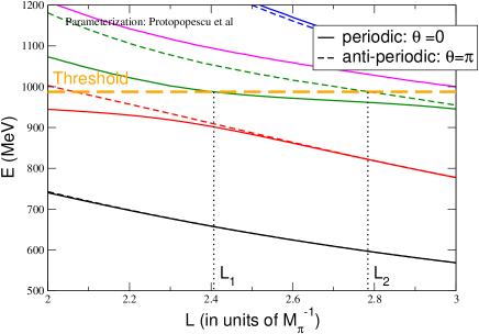
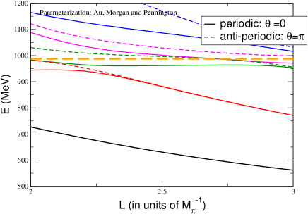
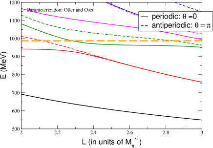
Figure 1: Energy levels $E_{n},~{}n=1,2,\cdots$ of the two-pion states in a finite box. Solid lines correspond to the periodic boundary conditions ($\theta=0$), and the dashed lines to the antiperiodic boundary conditions for the $s$-quark ($\theta=\pi$). Horizontal dashed line depicts the $K\bar{K}$ threshold. Different parameterizations of the $K$-matrix from Refs. [31, 30, 6] have been used.

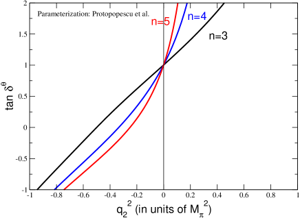
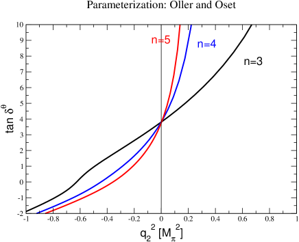
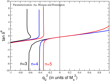
Figure 2: The tangent of the pseudophase in the vicinity of the $K\bar{K}$ threshold, in case of the periodic boundary conditions ($\theta=0$). The pseudophase was extracted from the excited energy levels $E_{n}$ with $n=3,4,5$. Different parameterizations have been used.

To summarize, with the above assumptions, the generalization of Eq. (1) to the finite-volume case is straightforward, and the result is similar in form to that given in Ref. [28]:

$$T_{ij}(s)=K_{ij}(s)+\frac{2}{\sqrt{\pi}L}\,\sum_{n}K_{in}(s)\,Z_{00}(1,k_{n}^{2})\,T_{nj}(s)\,,\quad\quad i,j,n=1,2\,,$$ (5)

where $k_{n}(s)=\dfrac{q_{n}(s)L}{2\pi}$ and $Z_{00}(1;k^{2})$ stands for Lüscher zeta-function [33, 26].

The equation (5) implies periodic boundary conditions on both pion and kaon fields. Below, we explore the possibility of using the so-called twisted boundary conditions, which we opt to impose only on the strange quark field, whereas $u$- and $d$-quarks obey periodic boundary conditions

$$u({\bf x}+L{\bf e}_{i})=u({\bf x})\,,\quad d({\bf x}+L{\bf e}_{i})=d({\bf x})\,,\quad s({\bf x}+L{\bf e}_{i})=\mbox{e}^{i\theta}s({\bf x})\,,\quad\quad 0\leq\theta<2\pi\,.$$ (6)

In this relation, ${\bf e}_{i},~{}i=1,2,3$ denote unit vectors along the lattice axes, and $V=L^{3}$ is the spatial volume of the lattice. The vacuum angle theta is chosen the same in all spatial directions, in order to avoid the breaking of the cubic symmetry. This choice, however, may be changed, if needed.

In the effective theory, the angle theta will appear in the boundary condition for the kaon field and not for the pion field.

$$K^{\pm}({\bf x}+L{\bf e}_{i})=\mbox{e}^{\mp i\theta}K^{\pm}({\bf x})\,,\quad K^{0}({\bf x}+L{\bf e}_{i})=\mbox{e}^{-i\theta}K^{0}({\bf x})\,,\quad\bar{K}^{0}({\bf x}+L{\bf e}_{i})=\mbox{e}^{i\theta}\bar{K}^{0}({\bf x})\,.$$ (7)

If $\theta\neq 0$, the $K\bar{K}$ pair at rest has the minimum relative momentum $\pm\biggl{(}\dfrac{\theta}{L},\dfrac{\theta}{L},\dfrac{\theta}{L}\biggr{)}$ and the energy $2\sqrt{M_{K}^{2}+\dfrac{3\theta^{2}}{L^{2}}}$. In other words, the $K\bar{K}$ threshold can be moved by adjusting $\theta$. Exactly this property makes the twisted boundary conditions particularly useful to study scalar mesons, which are located very close to this threshold.

Twisted boundary conditions can be straightforwardly implemented in the two-channel Lüscher equation (5). To this end, it suffices to replace $Z_{00}(1;k_{2}^{2})\to Z_{00}^{\theta}(1;k_{2}^{2})$, where

$$Z_{00}^{\theta}(1,k_{2}^{2})=\frac{1}{\sqrt{4\pi}}\lim_{s\to 1}\sum_{{\bf n}\in Z^{3}}\frac{1}{\left(\sum_{i=1}^{3}(n_{i}+\frac{\theta}{2\pi})^{2}\right)-k_{2}^{2}}\,,$$ (8)

whereas $Z_{00}(1;k_{1}^{2})$ stays put.

The energy levels are given by the secular equation, which is obtained from Eq. (5)

$$1-\frac{2}{\sqrt{\pi}L}\,Z_{00}(1;k_{1}^{2})\,K_{11}(s)-\frac{2}{\sqrt{\pi}L}\,Z_{00}^{\theta}(1;k_{2}^{2})\,K_{22}(s)$$ (9)

$$+ \frac{2}{\sqrt{\pi}L}\,Z_{00}(1;k_{1}^{2})\,\frac{2}{\sqrt{\pi}L}\,Z_{00}^{\theta}(1;k_{2}^{2})\,(K_{11}(s)K_{22}(s)-K_{12}(s)^{2})=0\,.$$

Our aim is to describe a procedure, which enables one to extract the $K$-matrix elements $K_{ij}$ in the vicinity of threshold from the lattice. We shall illustrate this procedure on the example of the synthetic data, which were produced, using different phenomenological parameterizations for the $\pi\pi$ S-wave phase shift and the Eq. (9) to determine the spectrum for various values of $\theta$. We have tested the parameterizations, given in Refs. [31, 30, 6] (these are shortly described in appendix A), and produced the spectrum which is shown in Fig. 1. In this figure, the spectra at $\theta=0$ (solid lines) and $\theta=\pi$ (dashed lines) are displayed. These spectra show quite similar behavior despite the fact that the pertinent $K$-matrices have very different properties. For example, the $K$-matrix from Ref. [30] has a real pole very close to the $K\bar{K}$ threshold, whereas the $K$-matrix from Refs. [31, 6] is regular near threshold. As expected, the spectrum is almost independent on the twist parameter $\theta$ away from threshold. Maximal variation is introduced in the vicinity of the threshold where the rearrangement of the levels occurs: the levels with $\theta=\pi$ for small values of $L$ are “pushed up” one level high as compared to the case with $\theta=0$. Consequently, the measurements for different values of $\theta$ provide an independent piece of information in the threshold region, where the $\theta$-dependence is maximal. Since we are looking for the resonances exactly in this region, twisted boundary conditions can be used to fix the location of these resonances. On the other hand, it is also clear from Fig. 1 that the attempts to identify separate levels with either the resonance or scattering states are not very informative. In particular, tuning the parameters $L,\theta$, one may easily move a single energy level above or below the threshold.

In order to facilitate the extraction of the $K$-matrix elements from the data, according to Ref. [28], it is convenient to define the pseudophase

$$\tan\delta^{\theta}(q_{1})=-\tan\phi(k_{1})\,,\quad\quad k_{1}=\frac{q_{1}L}{2\pi}\,,\quad\tan\phi(k_{1})=-\frac{\pi^{3/2}k_{1}}{Z_{00}(1;k_{1}^{2})}\,.$$ (10)

The ($\theta$-dependent) energy spectrum $q_{1}=q_{1}(L)$ can be (in principle) measured on the lattice. Consequently, the right-hand side of Eq. (10) (and, hence, the pseudophase) are measurables. The physical meaning of the pseudophase is the following: apply Lüscher formula to the measured energy spectrum, assuming that the scattering is elastic (in our case, this means that only $\pi\pi$ threshold is taken into account). Thus, below the inelastic $K\bar{K}$ threshold, the pseudophase coincides with the usual scattering phase. This is not the case above the inelastic threshold.

From Eq. (9) one may express the pseudophase through the $K$-matrix elements as follows:

$$\tan\delta^{\theta}(q_{1})=q_{1}\biggl{(}K_{11}(s)+\frac{\frac{2}{\sqrt{\pi}L}\,Z_{00}^{\theta}(1;k_{2}^{2})\,K_{12}(s)^{2}}{1-\frac{2}{\sqrt{\pi}L}\,Z_{00}^{\theta}(1;k_{2}^{2})\,K_{22}(s)}\biggr{)}\,.$$ (11)

Suppose, for a moment, that $\theta=0$ and we tuned the box size so that the energy is exactly equal to $2M_{K}$ (this corresponds to $L=L_{1}$ in Fig. 1) and measured the pseudophase for this box size. Recalling that $Z_{00}(1;k_{2}^{2})=-\dfrac{1}{\sqrt{4\pi}k_{2}^{2}}-2.514488997+O(k_{2}^{2})$ as $k_{2}^{2}\to 0$, from Eq. (11) we readily get

$$\lim_{k_{2}^{2}\to 0}\tan\delta^{\theta}(q_{1})\biggr{|}_{\theta=0}=\hat{q}_{1}\biggl{(}K_{11}^{(0)}-\frac{(K_{12}^{(0)})^{2}}{K_{22}^{(0)}}\biggr{)}\,.$$ (12)

This equation gives one relation between three quantities $K_{ij}^{(0)}$.

We repeat this procedure for a different value $L$ and adjust the parameter $\theta$ so that energy of the measured level is exactly $2M_{K}$ again. For example in Fig. 1 this corresponds to $L=L_{2}$ at $\theta=\pi$. After performing three measurements at threshold energy and different values of $L,\theta$, we get enough equations to determine all $K_{ij}^{(0)}$ separately. Moreover, there is nothing special about the threshold energy: the same procedure can be repeated at $\sqrt{s}\neq 2M_{K}$, scanning the matrix elements $K_{ij}(s)$ in the vicinity of threshold. In this way, one may e.g., answer the question, whether the $K$-matrix contains the pre-existing poles in the threshold region.

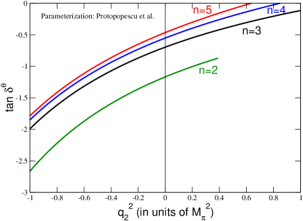
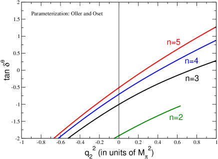
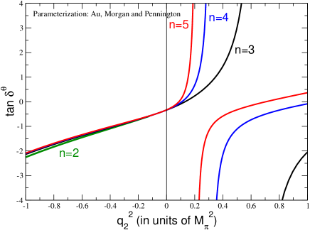
Figure 3: The same as in Fig. 2, but with antiperiodic boundary conditions $\theta=\pi$.

From Figs. 2 and 3 one may conclude that the difference between different parameterizations of the $K$-matrix is more clearly visible in the pseudophase that in the structure of the energy levels which all show a similar behavior. Moreover, it is seen that the behavior of the pseudophase changes dramatically when $\theta$ changes from $0$ to $\pi$. On the basis of this observation one may expect that the equations that relate the matrix elements $K_{ij}(s)$ with the measured pseudophases at the same energy are not degenerate and will enable one to neatly extract these matrix elements from the data.

Last but not least, we wish to comment on the relation of the approach suggested in the present paper with the method of HBC [21]. We shall do this, adapting the argumentation of Refs. [21] to a choice of the boundary conditions used in the present article. Namely, as already mentioned above, varying the parameter $\theta$ from $0$ to $\pi$ amounts to floating the $K\bar{K}$ threshold, whereas the $\pi\pi$ threshold stays put. Consequently, one interprets a given state as a $K\bar{K}$ scattering state if it is dragged along by the $K\bar{K}$ threshold, and as a “genuine quark state,” if it does not move. On the other hand, from the expression of the pseudophase Eq. (11) one may conclude that the energy level in the vicinity of the threshold does not move if the matrix element $K_{12}$ that describes the coupling of $\pi\pi$ and $K\bar{K}$ channels, is small. In terms of Flatté parameters, this corresponds to a small value of $g_{K}$, see Eq.4. In this case, a pair of poles appears in the $S$-matrix near the $K\bar{K}$ threshold. To summarize, it is seen that the approach proposed in the present paper is a natural generalization of the HBC method and enables one to extract and to quantify the information about the nature of the resonances in the threshold region.

Finally, we wish to mention that we performed the calculation of the energy levels and the pseudophases (for the different values of the twisting angle $\theta$) for the case of the $a_{0}(980)$ resonance as well, using the parameterization of Ref. [6]. The results turn out to be qualitatively similar to the case of the $f_{0}(980)$.

4 Strangeness content of the exotic states

As mentioned in the introduction, different methods are used at present to distinguish tetraquarks from ordinary $q\bar{q}$ mesons in lattice QCD. Usually, a state is said to be a tetraquark if it is seen in the two-point function of the operators $\bar{q}q\bar{q}q$ and not seen in the two-point function of the operators $\bar{q}q$. More precisely, this means that the overlap of the one particle state with the state produced from the vacuum by the operator $\bar{q}q\bar{q}q$ is much larger than with the state produced by the operator $q\bar{q}$. Furthermore, one may invoke arguments based on the behavior of the spectrum in quenched approximation [19]. However, one should take these arguments with a grain of salt. For example, the the matrix elements used in the above argumentation are scale-dependent and, in addition, depend on the way the operators are constructed from the quark fields. It is clear that a mathematically consistent and model-independent criterium would be highly desirable.

It should be pointed out that, generally speaking, the question whether the composition of a particular state is $q\bar{q}$ or $q^{2}\bar{q}^{2}$, makes sense e.g., in the non-relativistic quark models but not in the field theory. In the latter, any operator with appropriate quantum numbers can be used as an interpolating field for a given particle. Thus, we have to look for a criterium formulated in terms of observable quantities, which in the non-relativistic limit is coherent with our understanding of ordinary $q\bar{q}$ and tetraquark states. We shall use this strategy in the following.

Note first that the quark model wave functions of the states in the non-relativistic limit are eigenfunctions of the operator

$${\bf S}_{i}=\int d^{3}{\bf x}\,:\bar{q}_{i}(x)q_{i}(x):\,,\quad\quad i=u,d,s$$ (13)

with the eigenvalues $N_{i}+N_{\bar{i}}$, where $N_{i}$ and $N_{\bar{i}}$ denote the number of quarks and antiquarks of a flavor $i$ which are contained in this state.

Consider now the $SU(3)$ nonets with maximal mixing for the $q\bar{q}$ and $q^{2}\bar{q}^{2}$ mesons (the wave functions of the $q^{2}\bar{q}^{2}$ states are given, e.g., in Ref. [38]). Further, define the strangeness content of a state $B$ that belongs to these nonets in a standard manner

$$y_{B}=\frac{2\langle B|\bar{s}s|B\rangle}{\langle B|\bar{u}u+\bar{d}d|B\rangle}\,.$$ (14)

In the non-relativistic case, in order to calculate $y_{B}$, one has just to count the number of the quarks (antiquarks) of a given species in a state $B$. Using the wave functions from table 1, we may easily evaluate the values of $y_{B}$. The results are given in the same table.

$B$	$q\bar{q}$		$q^{2}\bar{q}^{2}$
$I=0$, nonstrange	$\frac{u\bar{u}+d\bar{d}}{\sqrt{2}}$,	$y_{B}=0$	$[ud][\bar{u}\bar{d}]$,	$y_{B}=0$
$I=0$, strange	$s\bar{s}$,	$y_{B}=\infty$	$\frac{[su][\bar{s}\bar{u}]+[sd][\bar{s}\bar{d}]}{\sqrt{2}}$,	$y_{B}=2$
$I=\frac{1}{2}$	$u\bar{s},~{}d\bar{s}\,+$ conj.,	$y_{B}=2$	$[su][\bar{u}\bar{d}],~{}[sd][\bar{u}\bar{d}]\,+$ conj.,	$y_{B}=\frac{2}{3}$
$I=1$	$u\bar{d},~{}\frac{u\bar{u}-d\bar{d}}{\sqrt{2}}\,~{}d\bar{u}$,	$y_{B}=0$	$[su][\bar{s}\bar{d}],~{}\frac{[su][\bar{s}\bar{u}]-[sd][\bar{s}\bar{d}]}{\sqrt{2}},~{}[sd][\bar{s}\bar{u}]$,	$y_{B}=2$

Table 1: The wave functions and the strangeness content of $q\bar{q}$ and $q^{2}\bar{q}^{2}$ mesons in the non-relativistic quark model with ideal mixing.

As one sees from table 1, the patterns followed by $y_{B}$ are very different for the $q\bar{q}$ mesons and tetraquarks. Note also that, in case of arbitrary mixing, these two nonets can be still distinguished due to the fact that $y_{B}$ for $I\neq 0$ does not depend on the mixing angle.

Next, we mention that the quantity $y_{B}$ is a well-defined quantity in QCD (it is scale-independent) and can be directly evaluated on the lattice e.g., by studying the quark mass dependence of the scalar meson masses and applying Feynman-Hellmann theorem

$$y_{B}=2\biggl{(}\frac{dM_{B}}{dm_{s}}\biggr{)}\cdot\biggl{(}\frac{dM_{B}}{d\hat{m}}\biggr{)}^{-1}\,,$$ (15)

where we have assumed that isospin is conserved: $m_{u}=m_{d}=\hat{m}$.

Now we are in a position to formulate our proposal. The quantity $y_{B}$ is a well-defined quantity in QCD and can be measured on the lattice. On the other hand, in the non-relativistic quark models this quantity clearly distinguishes between the $q\bar{q}$ and $q^{2}\bar{q}^{2}$ states. Therefore we can use the measured pattern of the quantity $y_{B}$ for the nonet states in order to define, what we understand under tetraquark states within relativistic quantum field theory. In contrast to the criteria used in the literature so far, this definition, e.g., does not operate with the quantities that are scale-dependent (like the matrix elements of multiquark operators). Note that we took advantage here of being able to vary quark masses on the lattice freely. Such a possibility is not available in the phenomenological approaches based on the experimental input and the above definition will be harder to use there.

Finally, note that the scalar mesons under consideration are resonances, not stable particles. Since the width of these resonances is very small, it is natural to continue using Eqs. (14) and (15). For example, $M_{B}$ in Eq. (15) is to be now understood as the resonance pole position. This means that the measured energy levels should be first “purified” with respect to the finite volume effects, as described in the previous sections. The method should be applied at the final stage, to the resonance poles extracted from the spectrum. If this is not done, the $K\bar{K}$ threshold, which will be moving if quark masses are varied, could strongly influence nearby energy levels, and this may result in wrong conclusions about the quark mass dependence of the true resonance energies.

Interestingly, the kaon mass dependence of the scalar mesons can also be used as a signature of the molecular picture. For a such a scenario, the leading Fock component of the scalar meson wave function has two quarks and two anti-quarks, much like the just discussed tetraquark states. However, while these are expected to be compact, a molecule is loosely bound and thus spatially extended. The molecular nature leads to a very peculiar kaon mass dependence of the molecule as shown in Ref. [39]. The mass of a $\bar{K}K$-molecule can be written as $M_{\rm mol}=M_{K}+M_{\bar{K}}-\epsilon$, with $\epsilon$ the small binding energy, $\epsilon\ll M_{K}$. Consequently, the kaon mass dependence of $M_{\rm mol}$ is expected to be linear with a slope of two, with correction of the order ${\cal O}(r^{2}\epsilon M_{\rm mol)}$, where $r$ denotes the range of forces. This is dramatically different from a tetraquark, where the kaon mass dependence is generated either from the strange valence or the strange sea quarks and is thus expected to depend on $m_{s}$ linearly or as $m_{s}^{3/2}$, generating a leading kaon mass dependence as $M_{K}^{2}$ or $M_{K}^{3}$, respectively. For a more detailed discussion on this issue, we refer to Ref. [39].

5 Conclusions

The main results of this investigation can be summarized as follows:

• Obviously, the measured excited spectrum can not be directly identified with the experimentally observed scalar mesons. This simple fact becomes crystal clear by looking at Fig. 1, where one has freely used the parameters $L$ and $\theta$ to move an energy level below or above $2M_{K}$. What defines the energy and the width of a resonance is the position of the $S$-matrix pole in the complex plane. This position can be determined, extracting $K$-matrix elements from the spectrum measured on the lattice.

• The procedure of determining $K$-matrix elements at the inelastic threshold, which was described in the present paper, is the generalization of Lüscher’s method to the elastic scattering length. It is also an improvement of the method described in Ref. [28]. Namely, using twisted boundary conditions, as proposed in the present paper, enables one to determine all three quantities $K_{ij}(s)$ in the vicinity of the inelastic threshold.

• Lüscher’s approach implies the study of the response of the energy spectrum on the variation of the box size $L$. We have shown that, for certain quantities, studying the dependence on the twisting angle $\theta$ may partly substitute studying the volume dependence. In other words, one may use the twisting parameter $\theta$ to scan the energy region in the vicinity of the $K\bar{K}$ threshold.

• The study of the $L$- and $\theta$-dependence of the energy spectrum of scalar mesons as proposed in the present paper is beyond any doubt a very demanding enterprise. The authors bear no illusion that the whole program can be realized in lattice calculations at physical quark masses anytime soon, especially for the $f_{0}(980)$ meson (the situation with $a_{0}(980)$ could be slightly better). However, we still find it important to formulate a rigorous way to treat the problem in question, which can be used one day.

• We show that the use of the twisted boundary conditions allows one to distinguish between the loosely bound molecular states and the compact quark compounds. We in addition argue that if the latter possibility is realized, the measured values of the strangeness content for the different members of the $SU(3)$ nonet allow one to interpret these states either as conventional $\bar{q}q$ states or $q^{2}\bar{q}^{2}$ tetraquark states. Thus the measurement of the strangeness content on the lattice, which can be achieved by studying the quark mass dependence of the resonance energies, enables one to gain detailed information about the structure of the scalar mesons. We have also pointed out that the molecular picture can be further tested from the measurement of the kaon mass dependence of the mass of the scalar mesons - for a molecular state this would be linear with slope two (modulo small corrections).

Acknowledgments. We would like to thank V. Baru, J. Gasser, C. Hanhart, B. Metsch, B. Moussallam, J. Oller, J. Pelaez, S. Prelovsek and C. Urbach for useful discussions. This work is supported in part by DFG (SFB/TR 16, “Subnuclear Structure of Matter”) and by the Helmholtz Association through funds provided to the virtual institute “Spin and strong QCD” (VH-VI-231). We also acknowledge the support of the European Community-Research Infrastructure Integrating Activity “Study of Strongly Interacting Matter” (acronym HadronPhysics2, Grant Agreement n. 227431) under the Seventh Framework Programme of EU. A.R. acknowledges support of the Georgia National Science Foundation (Grant #GNSF/ST08/4-401).

Appendix A Different parameterizations of the two-channel
$K$-matrix

A particular parameterization of the $K$-matrix elements from the paper Protopopescu et al., Ref. [31], which is used in the present paper, is given by

$$K_{ij}=(M^{-1})_{ij}\,,\quad\quad M_{ij}(s)=M_{ij}^{(0)}+(s-s_{t})M_{ij}^{(1)}\,,\quad\quad s_{t}=4M_{K}^{2}\,,$$ (A.1)

where the coefficients $M_{ij}^{(n)}$ take the following values

	$M_{11}^{(n)}$	$M_{12}^{(n)}$	$M_{22}^{(n)}$
$n=0$	$3.38\,M_{\pi}$	$2.40\,M_{\pi}$	$0.071\,M_{\pi}$
$n=1$	0	0	$-0.0038\,M_{\pi}^{-1}$

The scattering matrix in the paper by Oller and Oset, Ref. [6], is given by a solution of the 2-channel Bethe-Salpeter equation

$$T_{ij}(s)=V_{ij}(s)+\sum_{n}V_{in}(s)G_{n}(s)T_{nj}(s)\,,\quad\quad i,j,n=1,2\,,$$ (A.2)

where $V_{ij}(s)$ are the tree-level meson-meson scattering amplitudes, calculated in Chiral Perturbation Theory

$$V_{11}=-{\cal N}\,\frac{2s-M_{\pi}^{2}}{2F_{\pi}^{2}}\,,\quad V_{12}=V_{21}=-{\cal N}\,\frac{\sqrt{3}s}{4F_{\pi}^{2}}\,,\quad V_{22}=-{\cal N}\,\frac{3s}{4F_{\pi}^{2}},\quad{\cal N}=-(8\pi\sqrt{s})^{-1}$$ (A.3)

with $F_{\pi}\simeq 93~{}\mbox{MeV}$ and the loop functions $G_{k}(s)$ are given by

$$G_{n}={\cal N}^{-1}\biggl{\{}-\frac{1}{8\pi^{2}}\,\ln\frac{q^{\sf max}}{M_{n}}\biggl{(}1+\frac{w^{\sf max}_{n}}{q^{\sf max}}\biggr{)}+\frac{\sigma_{n}}{16\pi^{2}}\,\ln\frac{\sigma_{n}w^{\sf max}_{n}/q^{\sf max}+1}{\sigma_{n}w^{\sf max}_{n}/q^{\sf max}-1}\biggr{\}}\doteq G_{n}^{\sf R}+iq_{n}(s)\,.$$ (A.4)

In the above expression, $\sigma_{n}=\sqrt{1-\frac{4M_{n}^{2}}{s}+i0}$, $q^{\sf max}=\sqrt{\Lambda^{2}-M_{K}^{2}}$ is the cutoff momentum in the loops and $w^{\sf max}_{n}=\sqrt{M_{n}^{2}+(q^{\sf max})^{2}}$. The cutoff parameter $\Lambda$ is chosen to be $\Lambda\simeq 1020~{}\mbox{MeV}$.

The $K$-matrix elements are given by a solution of the equation

$$K_{ij}(s)=V_{ij}(s)+\sum_{n}V_{in}(s)G_{n}^{\sf R}(s)K_{nj}(s)\,.$$ (A.5)

In analogy to the parameterization by Protopopescu et al., the above $K$-matrix elements are regular in the vicinity of the $K\bar{K}$ threshold. The resonance emerges due to the rescattering effect.

In difference to this, the parameterization of the $K$-matrix in the paper by Au et al.,, Ref. [30] contains the pre-existing pole in the vicinity of the $K\bar{K}$ threshold. This parameterization looks as follows

$$K_{ij}=\frac{s-s_{0}}{4M_{K}^{2}}\,\biggl{\{}\frac{f_{i}f_{j}}{(s_{1}-s)(s_{1}-s_{0})}+\sum_{n=0}^{4}c^{n}_{ij}\biggl{(}\frac{s}{4M_{K}^{2}}-1\biggr{)}\biggr{\}}\,$$ (A.6)

where $s_{0}=-0.0162$, $s_{1}=0.9383$, $f_{1}=-0.1659$, $f_{2}=0.5852$ and the values of the coefficients $c^{n}_{ij}$ are given by

	$c_{11}^{n}$	$c_{12}^{n}$	$c_{22}^{n}$
$n=0$	0.4247	-3.1401	-2.8447
$n=1$	-0.5822	-0.1359	6.9164
$n=2$	2.5478	1.0286	5.2846
$n=3$	-1.7387	-2.3029	-0.9646
$n=4$	0.8308	0.1944	0

All dimensionful quantities are given in powers of GeV.

References

- [1] R. L. Jaffe, Phys. Rev. D 15 (1977) 267.
- [2] D. Black et al, Phys. Rev. D 59 (1999) 074026 [arXiv:hep-ph/9808415].
- [3] N. N. Achasov and A. V. Kiselev, Phys. Rev. D 68 (2003) 014006 [arXiv:hep-ph/0212153].
- [4] J. R. Pelaez, Mod. Phys. Lett. A 19 (2004) 2879 [arXiv:hep-ph/0411107].
- [5] J. D. Weinstein and N. Isgur, Phys. Rev. Lett. 48 (1982) 659.
- [6] J. A. Oller and E. Oset, Nucl. Phys. A 620 (1997) 438 [Erratum-ibid. A 652 (1999) 407] [arXiv:hep-ph/9702314];
- [7] J. A. Oller, E. Oset and J. R. Pelaez, Phys. Rev. Lett. 80 (1998) 3452 [arXiv:hep-ph/9803242]; J. A. Oller, E. Oset and J. R. Pelaez, Phys. Rev. D 59 (1999) 074001 [Erratum-ibid. D 60 (1999 ERRAT,D75,099903.2007) 099906] [arXiv:hep-ph/9804209].
- [8] J. A. Oller and E. Oset, Phys. Rev. D 60 (1999) 074023 [arXiv:hep-ph/9809337]; J. A. Oller, E. Oset and J. R. Pelaez, Phys. Rev. D 59 (1999) 074001 [Erratum-ibid. D 60 (1999 ERRAT,D75,099903.2007) 099906] [arXiv:hep-ph/9804209].
- [9] S. Peris, M. Perrottet and E. de Rafael, JHEP 9805 (1998) 011 [arXiv:hep-ph/9805442]; V. Elias, A. H. Fariborz, F. Shi and T. G. Steele, Nucl. Phys. A 633 (1998) 279 [arXiv:hep-ph/9801415].
- [10] G. Janssen, B. C. Pearce, K. Holinde and J. Speth, Phys. Rev. D 52 (1995) 2690 [arXiv:nucl-th/9411021].
- [11] S. Weinberg, Phys. Rev. 130 (1963) 776; Phys. Rev. 131 (1963) 440; Phys. Rev. 137 (1965) B672.
- [12] D. Morgan, Nucl. Phys. A 543 (1992) 632.
- [13] N. A. Törnqvist, Phys. Rev. D 51 (1995) 5312 [arXiv:hep-ph/9403234].
- [14] D. Morgan and M. R. Pennington, Phys. Lett. B 258 (1991) 444 [Erratum-ibid. B 269 (1991) 477]; Phys. Rev. D 48 (1993) 1185.
- [15] V. Baru, J. Haidenbauer, C. Hanhart, Yu. Kalashnikova and A. E. Kudryavtsev, Phys. Lett. B 586 (2004) 53 [arXiv:hep-ph/0308129].
- [16] V. Baru, J. Haidenbauer, C. Hanhart, A. E. Kudryavtsev and U.-G. Meißner, Eur. Phys. J. A 23 (2005) 523 [arXiv:nucl-th/0410099].
- [17] C. Hanhart, Eur. Phys. J. A 31 (2007) 543 [arXiv:hep-ph/0609136].
- [18] C. Hanhart, Eur. Phys. J. A 35 (2008) 271 [arXiv:0711.0578 [hep-ph]].
- [19] M. G. Alford and R. L. Jaffe, Nucl. Phys. B 578 (2000) 367 [arXiv:hep-lat/0001023].
- [20] T. Kunihiro, S. Muroya, A. Nakamura, C. Nonaka, M. Sekiguchi and H. Wada [SCALAR Collaboration], Phys. Rev. D 70 (2004) 034504 [arXiv:hep-ph/0310312].
- [21] F. Okiharu et al., arXiv:hep-ph/0507187; H. Suganuma, K. Tsumura, N. Ishii and F. Okiharu, PoS LAT2005 (2006) 070 [arXiv:hep-lat/0509121]; Prog. Theor. Phys. Suppl. 168 (2007) 168 [arXiv:0707.3309 [hep-lat]].
- [22] N. Mathur et al., Phys. Rev. D 76 (2007) 114505 [arXiv:hep-ph/0607110].
- [23] C. McNeile and C. Michael [UKQCD Collaboration], Phys. Rev. D 74 (2006) 014508 [arXiv:hep-lat/0604009]; A. Hart, C. McNeile, C. Michael and J. Pickavance [UKQCD Collaboration], Phys. Rev. D 74 (2006) 114504 [arXiv:hep-lat/0608026].
- [24] H. Wada, T. Kunihiro, S. Muroya, A. Nakamura, C. Nonaka and M. Sekiguchi, Phys. Lett. B 652 (2007) 250 [arXiv:hep-lat/0702023].
- [25] S. Prelovsek, C. Dawson, T. Izubuchi, K. Orginos and A. Soni, Phys. Rev. D 70 (2004) 094503 [arXiv:hep-lat/0407037]; S. Prelovsek, T. Draper, C. B. Lang, M. Limmer, K. F. Liu, N. Mathur and D. Mohler, arXiv:1002.0193 [hep-ph]; arXiv:1005.0948 [hep-lat].
- [26] M. Lüscher, Nucl. Phys. B 354 (1991) 531.
- [27] P. F. Bedaque, Phys. Lett. B 593 (2004) 82 [arXiv:nucl-th/0402051]. G. M. de Divitiis, R. Petronzio and N. Tantalo, Phys. Lett. B 595 (2004) 408 [arXiv:hep-lat/0405002]. G. M. de Divitiis and N. Tantalo, arXiv:hep-lat/0409154. C. T. Sachrajda and G. Villadoro, Phys. Lett. B 609 (2005) 73 [arXiv:hep-lat/0411033].
- [28] M. Lage, U.-G. Meißner and A. Rusetsky, Phys. Lett. B 681 (2009) 439 [arXiv:0905.0069 [hep-lat]].
- [29] V. Bernard, M. Lage, U. G. Meissner and A. Rusetsky, JHEP 0808 (2008) 024 [arXiv:0806.4495 [hep-lat]].
- [30] K. L. Au, D. Morgan and M. R. Pennington, Phys. Rev. D 35 (1987) 1633.
- [31] S. D. Protopopescu et al., Phys. Rev. D 7 (1973) 1279.
- [32] S. M. Flatte, Phys. Lett. B 63 (1976) 224.
- [33] M. Lüscher, Commun. Math. Phys. 105 (1986) 153.
- [34] D. Hoja, U.-G. Meißner and A. Rusetsky, arXiv:1001.1641 [hep-lat].
- [35] U.-G. Meißner, K. Polejaeva and A. Rusetsky, arXiv:1007.0860 [hep-lat].
- [36] C. Liu, X. Feng and S. He, Int. J. Mod. Phys. A 21 (2006) 847 [arXiv:hep-lat/0508022].
- [37] J. R. Pelaez and F. J. Yndurain, Phys. Rev. D 71 (2005) 074016 [arXiv:hep-ph/0411334].
- [38] G. ’t Hooft, G. Isidori, L. Maiani, A. D. Polosa and V. Riquer, Phys. Lett. B 662 (2008) 424 [arXiv:0801.2288 [hep-ph]].
- [39] M. Cleven, F. K. Guo, C. Hanhart and U.-G. Meißner, arXiv:1009.3804 [hep-ph].