Spin effects in transport through single-molecule magnets in the sequential and cotunneling regimes

Abstract

We analyze the stationary spin-dependent transport through a single-molecule magnet weakly coupled to external ferromagnetic leads. Using the real-time diagrammatic technique, we calculate the sequential and cotunneling contributions to current, tunnel magnetoresistance and Fano factor in both linear and nonlinear response regimes. We show that the effects of cotunneling are predominantly visible in the blockade regime and lead to enhancement of tunnel magnetoresistance (TMR) above the Julliere value, which is accompanied with super-Poissonian shot noise due to bunching of inelastic cotunneling processes through different virtual spin states of the molecule. The effects of external magnetic field and the role of type and strength of exchange interaction between the LUMO level and the molecule’s spin are also considered. When the exchange coupling is ferromagnetic, we find an enhanced TMR, while in the case of antiferromagnetic coupling we predict a large negative TMR effect.

I Introduction

Owing to recent advances in experimental techniques, it is now possible to study transport properties of individual nanoscale objects, like quantum dots, van der Wiel et al. (2002) nanotubes,Tans et al. (1997, 1998); Tsukagoshi et al. (1999); Cleuziou et al. (2006) and other molecules. Reed et al. (1997); Porath et al. (1997, 2000); Park et al. (2000); Reichert et al. (2002); Grose et al. (2008) Investigation of electron transport through molecules is stimulated by the prospect of a new generation of molecule-based electronic and spintronic devices. It turns out that owing to their unique optical, magnetic and mechanical properties, molecules are ideal candidates for constructing novel hybrid devices of functionality which would be rather hardly accessible in the case of conventional silicon-based electronic systems. Joachim et al. (2000); Nitzan and Ratner (2003); Tao (2006); Bogani and Wernsdorfer (2008) For instance, one interesting feature of nanomolecular systems, which does not have counterpart in bulk materials, concerns the interplay between the quantized electronic and mechanical degrees of freedom. Park et al. (2000)

In this paper we deal with one specific class of molecules which possess an intrinsic magnetic moment, referred to as single-molecule magnets (SMMs). Caneschi et al. (1999); Christou et al. (2000); Gatteschi et al. (2006) Such molecules are characterized by a significant Ising-like magnetic anisotropy and a high spin number $S$, which give rise to an energy barrier that the molecule has to overcome to reverse its spin orientation. At higher temperatures, the SMM’s spin can freely rotate, whereas below a certain temperature it becomes trapped in one of two metastable orientations. Since magnetic bistability is one of the key properties to be utilized in information processing technologies, SMMs have attracted much attention and a great deal of effort was undertaken to measure electronic transport through a SMM. Heersche et al. (2006); Ni et al. (2006); Jo et al. (2006); Henderson et al. (2007); Voss et al. (2008) The experiments carried out to date have concerned only the case of SMMs coupled to nonmagnetic electrodes. However, it has been suggested recently that spin-polarized currents (when the leads are ferromagnetic, for instance) can be used to manipulate the magnetic state of a SMM. Misiorny and Barnaś (2007a, b); Timm and Elste (2006); Elste and Timm (2006); Misiorny and Barnaś (2009a) Such a current-induced magnetic switching (CIMS) of a SMM takes place as a consequence of the angular momentum transfer between the molecule and conduction electrons.

When considering coupling strength between the molecule and external leads, one can generally distinguish between weak and strong coupling regimes. In the latter case, i.e. when resistance of the contact between the molecule and electrodes becomes smaller than the quantum resistance, the electronic correlations may lead to formation of the Kondo effect. Romeike et al. (2006a, b); Leuenberger and Mucciolo (2006); Roosen et al. (2008); Gonzalez et al. (2008) These correlations result in a screening of the SMM’s spin by conduction electrons of the leads, giving rise to a peak in the density of states and full transparency through the molecule. On the other hand, in the weak coupling regime, the Coulomb correlations lead to blockade phenomena. Grabert (1992) For voltages lower than a certain threshold value, sequential tunneling processes through the molecule are then exponentially suppressed due to Coulomb correlations and/or size quantization. However, once the bias voltage exceeds the threshold value, the electrons can tunnel one-by-one through the molecule. The latter regime is known as the sequential tunneling regime, and the former one is often referred to as the Coulomb blockade or cotunneling regime. Averin and Odintsov (1989); Averin and Nazarov (1990) It should be noted, however, that although the sequential processes are suppressed in the Coulomb blockade regime, current still can flow due to second- and higher-order tunneling processes, which involve correlated tunneling through virtual states of the molecule. Furthermore, although higher-order processes play a substantial role mainly in the cotunneling regime, they remain active in the whole range of transport voltages, especially on resonance, leading to renormalization of the molecule levels and smearing of the Coulomb steps. König (1999) Therefore a suitable theoretical method should be used to properly investigate transport through molecules in the regime where both the sequential and cotunneling processes coexist and determine transport properties. The existing analytical studies of electronic transport through SMMs in the weak coupling regime were based on the standard perturbation approach, Misiorny and Barnaś (2007b); Timm and Elste (2006); Misiorny and Barnaś (2009a); Elste and Timm (2006); Misiorny and Barnaś (2009b, c) and they dealt separately either with the sequential or cotunneling regime, with one attempt of combining them. Elste and Timm (2007) Nevertheless, to properly take into account the nonequilibrium many-body effects such as for example on-resonance level renormalization or level splitting due to an effective exchange field, simple rate equation arguments are not sufficient.

The main objective of the present paper is thus a systematic analysis of charge and spin transport through a SMM. This has been achieved by employing the real-time diagrammatic technique, Schoeller and Schön (1994) which enables accurate study of transport properties in the full weak coupling regime. In particular, including the first- and second-order self-energy diagrams, we calculate the current, tunnel magnetoresistance (TMR) and shot noise in the presence of sequential tunneling, cotunneling and cotunneling-assisted sequential tunneling processes. We show that the second-order processes determine transport in the Coulomb blockade regime, leading for instance to enhanced tunnel magnetoresistance effect as compared to the value based on the Julliere model, Julliere (1975) and to super-Poissonian shot noise due to bunching of inelastic cotunneling processes through the molecule. In addition, we also discuss the effects due to external magnetic field as well as the role of strength and type of exchange interaction between the molecule’s spin and conduction electrons.

The paper is organized as follows. In section II we describe the model of a single-molecule magnet coupled to ferromagnetic leads. The real-time diagrammatic technique used in calculations is presented briefly in section III. Section IV is devoted to numerical results and their discussion. In particular, the conductance, tunnel magnetoresistance and shot noise in the linear and nonlinear response regimes are analyzed in subsections A and B, respectively. The dependence of transport properties on the strength of exchange coupling is discussed in subsection C, while the effects of longitudinal external magnetic field are considered in subsection D. Furthermore, we also briefly discuss transport characteristics in the case when the exchange coupling is antiferromagnetic, subsection E. Finally, conclusions are given in section V.

II Description of model

In this paper we consider a model SMM which is attached to two metallic ferromagnetic electrodes, see Fig. 1. The molecule is assumed to be weakly coupled to the leads, whose magnetizations form a collinear configuration, either parallel or antiparallel. The limit of strong coupling, where interesting phenomena such as the Kondo effect Romeike et al. (2006a, b); Leuenberger and Mucciolo (2006); Roosen et al. (2008); Gonzalez et al. (2008) can be observed, is not considered here.

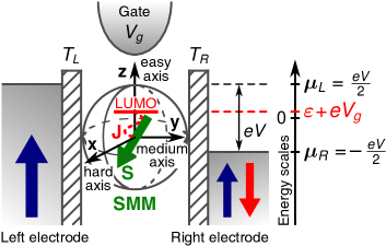
Figure 1: (color online) Schematic representation of the system under consideration. The system consists of a SMM weakly coupled to two ferromagnetic electrodes with the collinear configuration of their magnetic moments, i.e. either parallel or antiparallel. Due to symmetrically applied bias voltage $V=(\mu_{L}-\mu_{R})/e$, where $\mu_{L(R)}$ denotes the electrochemical potential of the left (right) lead, the LUMO level is independent of $V$. Position of the LUMO level, however, can be tuned by the gate voltage $V_{g}$.

Electronic transport through the molecule is assumed to take place only via the lowest unoccupied molecular orbital (LUMO) of the SMM, which is coupled to the internal magnetic core of the molecule via exchange interaction. Moreover, we also neglect all other unoccupied levels which are assumed to be well above the LUMO level and therefore cannot take part in transport for voltages of interest. Misiorny and Barnaś (2009a) Furthermore, following previous theoretical studies, Misiorny and Barnaś (2007a, b); Timm and Elste (2006); Elste and Timm (2006) we restrict our considerations to the case of molecules with vanishingly small transverse anisotropy.

Taking the above into account, a SMM coupled to external leads can be described by Hamiltonian of the general form

$$\mathcal{H}=\mathcal{H}_{\textrm{SMM}}+\mathcal{H}_{\textrm{leads}}+\mathcal{H}_{\textrm{T}}\,.$$ (1)

The first term on the right hand side describes the SMM and is assumed in the following form:

$$\mathcal{H}_{\textrm{SMM}}= -\Big{[}D+\sum_{\sigma}D_{1}\,c_{\sigma}^{\dagger}c_{\sigma}+D_{2}\,c_{\uparrow}^{\dagger}c_{\uparrow}c_{\downarrow}^{\dagger}c_{\downarrow}\Big{]}S_{z}^{2}$$

$$+\sum_{\sigma}\varepsilon\,c_{\sigma}^{\dagger}c_{\sigma}+U\,c_{\uparrow}^{\dagger}c_{\uparrow}c_{\downarrow}^{\dagger}c_{\downarrow}-J\textbf{s}\cdot\textbf{S}$$

$$+g\mu_{\textrm{B}}(S_{z}+s_{z})H_{z}.$$ (2)

The first line of Eq. (II) accounts for the uniaxial magnetic anisotropy of a SMM, characterized by the uniaxial anisotropy constant $D$ of a free-standing (neutral) molecule. When a bias voltage is applied, the LUMO level can be charged with up to two electrons, which in turn can affect the magnitude of the uniaxial anisotropy. The relevant corrections are included by the constants $D_{1}$ and $D_{2}$. Moreover, $S_{z}$ denotes the $z$ component of the internal (core) spin operator S, whereas $c_{\sigma}^{\dagger}$ $(c_{\sigma})$ is the creation (annihilation) operator of an electron in the LUMO level. We note that the Hamiltonian (2) is applicable to situations where electronic structure of the molecules’s magnetic core is not changed by adding one or two electrons to the LUMO level, except for modification of the anisotropy constants.

The second line of the Hamiltonian $\mathcal{H}_{\textrm{SMM}}$ describes the LUMO level of energy $\varepsilon$, with $U$ being the Coulomb energy of two electrons of opposite spins that can occupy this level. Although the position of the LUMO level can be modified by the gate voltage $V_{g}$, it remains independent of the symmetrically applied bias voltage $V$. An important term for the present discussion is the last one, given explicitly by

$$J\textbf{s}\cdot\textbf{S}=\frac{J}{2}c_{\uparrow}^{\dagger}c_{\downarrow}S_{-}+\frac{J}{2}c_{\downarrow}^{\dagger}c_{\uparrow}S_{+}+\frac{J}{2}\Big{[}c_{\uparrow}^{\dagger}c_{\uparrow}-c_{\downarrow}^{\dagger}c_{\downarrow}\Big{]}S_{z}\,,$$ (3)

which stands for exchange coupling between the magnetic core of a SMM, represented by the spin S, and electrons in the LUMO level, described by the local spin operator $\textbf{s}=\frac{1}{2}\sum_{\sigma\sigma^{\prime}}c_{\sigma}^{\dagger}\bm{\sigma}_{\sigma\sigma^{\prime}}c_{\sigma^{\prime}}$, where $\bm{\sigma}$ is the vector of Pauli matrices. This interaction can be either of ferromagnetic ($J>0$) or antiferromagnetic ($J<0$) type. Finally, the last term of $\mathcal{H}_{\textrm{SMM}}$ describes the Zeeman splitting associated with the magnetic field applied along the easy axis of the molecule, where $g$ stands for the Landé factor, and $\mu_{\textrm{B}}$ is the Bohr magneton.

In general, the molecular Hamiltonian $\mathcal{H}_{\textrm{SMM}}$ is not diagonal, except for the case of a free-standing (uncharged) uniaxial SMM. It has been shown Timm and Elste (2006); Misiorny and Barnaś (2007b, 2009a) that for the molecules with no transverse anisotropy, $\mathcal{H}_{\textrm{SMM}}$ commutes with the $z$th component ($S_{t}^{z}$) of the total spin $\textbf{S}_{t}\equiv\textbf{S}+\textbf{s}$, hence allowing us to analytically diagonalize it in the basis represented by the eigenvalues $m$ of $S_{t}^{z}$ and the corresponding occupation number $n$ of the LUMO level. In a general case, on the other hand, the problem can be dealt with numerically by performing a unitary transformation $U^{\dagger}\mathcal{H}_{\textrm{SMM}}U=\widetilde{\mathcal{H}}_{\textrm{SMM}}$ to a new basis in which $\widetilde{\mathcal{H}}_{\textrm{SMM}}$ is diagonal. Consequently, we obtain the set of relevant eigenvectors $|\chi\rangle$ and the corresponding eigenvalues $\varepsilon_{\chi}$ satisfying $\widetilde{\mathcal{H}}_{\textrm{SMM}}|\chi\rangle=\varepsilon_{\chi}|\chi\rangle$.

The second term of Eq. (1) describes ferromagnetic electrodes, and the $q$th electrode ($q=L,R$) is characterized by noninteracting itinerant electrons with the dispersion relation $\varepsilon_{\textbf{k}\sigma}^{q}$, where k denotes a wave vector and $\sigma$ is the electron’s spin. As a result, the lead Hamiltonian can be written as

$$\mathcal{H}_{\textrm{leads}}=\sum_{q}\sum_{\textbf{k},\sigma}\varepsilon_{\textbf{k}\sigma}^{q}\>a_{\textbf{k}\sigma}^{q{\dagger}}a_{\textbf{k}\sigma}^{q}\,,$$ (4)

where $a_{\textbf{k}\sigma}^{q{\dagger}}$ ($a_{\textbf{k}\sigma}^{q}$) is the creation (annihilation) operator for an electron in the $q$th electrode. The degree of spin polarization of the ferromagnetic lead $q$ can be described by the parameter $P_{q}$, $P_{q}=(D_{+}^{q}-D_{-}^{q})/(D_{+}^{q}+D_{-}^{q})$, with $D_{\pm}^{q}$ denoting the density of states for majority (upper sign) and minority (lower sign) electrons at the Fermi level in the lead $q$.

Finally, the last term $\mathcal{H}_{\textrm{T}}$ of the total Hamiltonian (1) describes tunneling processes between the molecule and the leads, and it is given by

$$\mathcal{H}_{\textrm{T}}=\sum_{q}\sum_{\textbf{k},\sigma}\Big{[}T_{q}\,a_{\textbf{k}\sigma}^{q{\dagger}}c_{\sigma}+T_{q}^{*}c_{\sigma}^{\dagger}a_{\textbf{k}\sigma}^{q}\Big{]}\,,$$ (5)

with $T_{q}$ denoting the tunnel matrix element between the molecule and the $q$th lead. Due to the tunneling processes, the LUMO level of the molecule acquires a finite spin-dependent width, $\Gamma_{\sigma}=\sum_{q}\Gamma_{\sigma}^{q}$, where $\Gamma_{\sigma}^{q}=2\pi|T_{q}|^{2}D_{\sigma}^{q}$. The parameters $\Gamma^{q}_{\pm}$ can be also expressed in terms of the spin polarization $P_{q}$ of the lead $q$ as $\Gamma^{q}_{\pm}=\Gamma_{q}(1\pm P_{q})$ for spin-majority (upper sign) and spin-minority (lower sign) electrons, where $\Gamma_{q}=(\Gamma^{q}_{+}+\Gamma^{q}_{-})/2$. In the following these parameters will be used to describe the strength of coupling between the LUMO level and the leads. Unless stated otherwise, the couplings are assumed to be symmetric, $\Gamma_{\rm L}=\Gamma_{\rm R}=\Gamma/2$.

III Method of calculations

Among different available methods, only a few enable us to analyze spin-dependent transport of the considered system in both the sequential and Coulomb blockade regimes within one fully consistent theoretical approach. Timm (2008) In particular, here, we employ the real-time diagrammatic technique, Schoeller and Schön (1994); König et al. (1996); König (1999); Thielmann et al. (2003, 2005); Weymann et al. (2005) which has already proven its reliability and versatility in studying transport properties of various nanoscopic systems.

The basic idea of this technique relies on a systematic perturbation expansion of the reduced density matrix of the system under discussion and the operators of interest with respect to the coupling strength $\Gamma$ between the LUMO level and the leads. All quantities, such as the current $I$, differential conductance $G$ and the (zero-frequency) current noise $S$ are essentially determined by the nonequilibrium time evolution of the reduced density matrix for the molecule’s degrees of freedom. In the case considered in this paper, the density matrix has only diagonal matrix elements, $p_{\chi}(t)$, which correspond to probability of finding the molecule in state $|\chi\rangle$ at time $t$. Following the matrix notation introduced by Thielmann et al., Thielmann et al. (2003) the vector $\textbf{p}(t)$ of the probabilities is given by the relation Schoeller and Schön (1994); König et al. (1996); König (1999)

$$\textbf{p}(t)=\bm{\Pi}(t,t_{0})\textbf{p}(t_{0})\,,$$ (6)

where $\bm{\Pi}(t,t_{0})$ is the propagator matrix whose elements, $\Pi_{\chi^{\prime}\chi}(t,t_{0})$, describe the time evolution of the system that propagates from a state $|\chi\rangle$ at time $t_{0}$ to a state $|\chi^{\prime}\rangle$ at time $t$, and $\textbf{p}(t_{0})$ is a vector representing the distribution of initial probabilities. In principle, the whole dynamics of the system is governed by the time evolution of the reduced density matrix. Furthermore, this time evolution can be schematically depicted as a sequence of irreducible diagrams on the Keldysh contour, König (1999) which after summing up correspond to irreducible self-energy blocks $W_{\chi^{\prime}\chi}(t^{\prime},t)$. Thielmann et al. (2003) The self-energy matrix $\textbf{W}(t^{\prime},t)$ is therefore one of the central quantities of the real-time diagrammatic technique, as its elements $W_{\chi^{\prime}\chi}(t^{\prime},t)$ can be interpreted as generalized transition rates between two arbitrary molecular states: $|\chi\rangle$ at time $t$ and $|\chi^{\prime}\rangle$ at time $t^{\prime}$. Consequently, the Dyson equation for the propagator is obtained in the form König (1999); Thielmann et al. (2003); Schoeller and Schön (1994); König et al. (1996)

$$\bm{\Pi}(t,t_{0})=\textbf{1}+\int_{t_{0}}^{t}\textrm{d}t_{2}\int_{t_{0}}^{t_{2}}\textrm{d}t_{1}\textbf{W}(t_{2},t_{1})\bm{\Pi}(t_{1},t_{0})\,.$$ (7)

By multiplying Eq. (7) from the right hand side with $\textbf{p}(t_{0})$, and differentiating it with respect to time $t$, one gets the general kinetic equation for the probability vector $\textbf{p}(t)$,

$$\frac{\textrm{d}}{\textrm{d}t}\textbf{p}(t)=\int_{t_{0}}^{t}\textrm{d}t_{1}\textbf{W}(t,t_{1})\textbf{p}(t_{1})\,.$$ (8)

In the limit of stationary transport the aforementioned formula reduces to the steady state master-like equation Schoeller and Schön (1994); Thielmann et al. (2003); König et al. (1996); König (1999)

$$\Big{(}\widetilde{\textbf{W}}\textbf{p}^{\textrm{st}}\Big{)}_{\chi}=\Gamma\delta_{\chi\chi_{0}}\,,$$ (9)

where $\textbf{p}^{\textrm{st}}=\lim_{t\rightarrow\infty}\textbf{p}(t)=\lim_{t_{0}\rightarrow-\infty}\textbf{p}(0)$ is the stationary probability vector, independent of initial distribution. On the other hand, $\widetilde{\textbf{W}}$ denotes the Laplace transform of the self-energy matrix $\textbf{W}(t^{\prime},t)$, whose one arbitrary row $\chi_{0}$ has been replaced with $(\Gamma,\ldots,\Gamma)$ to include the normalization condition for the probabilities $\sum_{\chi}p_{\chi}^{\textrm{st}}=1$. Knowing the probabilities, the electric current flowing through the system can be calculated from the formula Thielmann et al. (2003)

$$I=\frac{e}{2\hbar}\textrm{Tr}\left[\textbf{W}^{I}\textbf{p}^{st}\right]\,,$$ (10)

where the matrix $\textbf{W}^{I}$ denotes the self-energy matrix in which one internal vertex originating from the expansion of tunneling Hamiltonian $\mathcal{H}_{\textrm{T}}$ has been substituted with an external vertex for the current operator.

In order to calculate the transport quantities in both the deep Coulomb blockade and the sequential tunneling regime in each order in tunneling processes, we perform the perturbation expansion in $\Gamma$ adopting the so-called crossover perturbation scheme, Weymann et al. (2005) i.e. we expand the self-energy matrices, $\widetilde{\textbf{W}}=\sum_{n=1}^{\infty}\widetilde{\textbf{W}}^{\raisebox{-4.0pt}{\scalebox{0.7}{(n)}}}$ and $\textbf{W}^{I}=\sum_{n=1}^{\infty}\textbf{W}^{I(n)}$. Here, the first order of expansion ($n=1$) corresponds to sequential tunneling processes, while the second-order contribution ($n=2$) is associated with cotunneling processes. In the present calculations we take into account both the first- and second-order diagrams, which allows us to resolve the transport properties in the full weak coupling regime, i.e. in the cotunneling as well as in the sequential tunneling regimes. Furthermore, by considering the $n=1$ and $n=2$ terms of the expansion, we systematically include the effects of LUMO level renormalization, cotunneling-assisted sequential tunneling, as well as effects associated with an exchange field exerted by ferromagnetic leads on the molecule. König and Martinek (2003); Weymann et al. (2005); Weymann and Barnaś (2007) For $n\leq 2$, the stationary probabilities can be found from Eq. (9), with $\widetilde{\textbf{W}}=\widetilde{\textbf{W}}^{\raisebox{-4.0pt}{\scalebox{0.7}{(1)}}}+\widetilde{\textbf{W}}^{\raisebox{-4.0pt}{\scalebox{0.7}{(2)}}}$. On the other hand, the current is explicitly given by Eq. (10) where one has to take $\textbf{W}^{I}=\textbf{W}^{I(1)}+\textbf{W}^{I(2)}$. The key problem is now the somewhat lengthy but straightforward calculation of the respective self-energy matrices, which can be done using the corresponding diagrammatic rules. Schoeller and Schön (1994); König et al. (1996); König (1999); Thielmann et al. (2003); Weymann et al. (2005) An example of explicit formula for a second-order self-energy between arbitrary states $|\chi\rangle$ and $|\chi^{\prime}\rangle$ can be found in Ref. [Weymann, 2008].

With recent progress in detection of ultra-small signals, it has become clear that the information about the system transport properties can also be extracted from the measurement of current noise. Blanter and Büttiker (2000) In fact, the shot noise contains information about various correlations, coupling strengths, effective charges, etc., which is sometimes unaccessible just from measurements of electric current. Therefore, to make the analysis more self-contained, in this paper we will also calculate and discuss the zero-frequency shot noise. The shot noise is usually defined as the correlation function of the current operators, and its Fourier transform in the limit of low frequencies is given by Blanter and Büttiker (2000) $S=2\int_{-\infty}^{0}\textrm{d}t\big{[}\big{\langle}I(t)I(0)+I(0)I(t)-2\langle I\rangle^{2}\big{\rangle}\big{]}$. For $|eV|>k_{\rm B}T$, the current noise is dominated by fluctuations associated with the discrete nature of charge (shot noise), while for low bias voltages, the thermal noise dominates. Blanter and Büttiker (2000) The general formula for the current noise within the language of real-time diagrammatic technique can be found in Ref. [Thielmann et al., 2005].

IV Numerical results and discussion

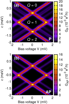
Figure 2: (color online) The total (first plus second order) differential conductance in the parallel (a) and antiparallel (b) configurations for the parameters: $S=2$, $J=0.2$ meV, $D=0.05$ meV, $D_{1}=-0.005$ meV, $D_{2}=0.002$ meV, $U=1$ meV, $k_{\rm B}T=0.04$ meV, $P_{L}=P_{R}=0.5$, and $\Gamma=0.002$ meV.

In this section we present and discuss numerical results on charge current, differential conductance, shot noise (Fano factor) and tunnel magnetoresistance (TMR) in the linear and nonlinear response regimes. The Fano factor

$$F=\frac{S}{2e|I|}\,,$$ (11)

describes deviation of the current noise from its Poissonian value, $S_{P}=2e|I|$, which is characteristic of uncorrelated in time tunneling processes. On the other hand, the TMR is defined as Julliere (1975); Barnaś and Fert (1998); Weymann et al. (2005)

$${\rm TMR}=\frac{I_{\rm P}-I_{\rm AP}}{I_{\rm AP}}\,,$$ (12)

where $I_{\rm P}$ ($I_{\rm AP}$) is the current flowing through the system in the parallel (antiparallel) magnetic configuration at a constant bias voltage $V$. The TMR describes a change of transport properties when magnetic configuration of the device varies from antiparallel to parallel alignment – the conductance is usually larger in the parallel configuration and smaller in the antiparallel one, although opposite situation is also possible.

Numerical results have been obtained for a hypothetical SMM characterized by the spin number $S=2$ and strong uniaxial magnetic anisotropy. However, we note that although in the following we assume $S=2$, our considerations are still quite general and qualitatively valid for molecules with larger spin numbers. In fact, the choice of low molecule’s spin allows us to perform a detailed analysis of various molecular states mediating the first and second-order tunneling processes. A large number of molecular states for $S\gg 1$ would make the discussion rather obscure. Apart from this, we assume a symmetrical coupling of the molecule to the two external leads ($P_{L}=P_{R}=P$) and ferromagnetic exchange coupling between the molecule’s magnetic core and electrons in the LUMO level. Later on, however, we will relax the latter restriction and consider the situation where the exchange coupling is antiferromagnetic. For clarity reasons, we disregard the effects due to the negative sign of electron charge, i.e. assume that charge current and particle (electron) current flow in the same direction ($e>0$).

We start from some basic transport characteristics of the system under consideration. In Fig. 2 we show the differential conductance in the parallel and antiparallel configurations as a function of the bias voltage and position of the LUMO level. The latter can be experimentally changed by sweeping the gate voltage. The density plot of the conductance displays the well-known Coulomb diamond pattern. The average charge accumulated in the LUMO level is $Q=\sum_{\chi}n(\chi)p_{\chi}^{\textrm{st}}$ (in the units of $e$), where $n(\chi)=0,1,2$ denotes the number of additional electrons on the molecule in the state $|\chi\rangle$. When lowering energy of the LUMO level, the latter becomes consecutively occupied with electrons. This leads to two peaks in the linear conductance, separated approximately by $U$, which correspond to single and double occupancy, respectively, see Fig. 2 for $V=0$.

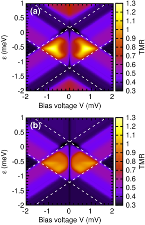
Figure 3: (color online) Density plot of the total (first plus second order) TMR (a) and TMR calculated in the sequential tunneling approximation (b) plotted in the same scale and for the same parameters as in Fig. 2. The sequential TMR is smaller than the total TMR. The dashed lines are only a guide for eyes, and they represent positions of the main conductance peaks, Fig. 2, separating thus regions corresponding to different occupation states of the LUMO level.

Furthermore, in the nonlinear response regime, the differential conductance shows additional lines due to tunneling through excited states of the molecule. These features are visible in both magnetic configurations. On the other hand, the hallmark of spin-depended tunneling is the difference in magnitude of the conductance in parallel and antiparallel configurations – the conductance in the parallel configuration is generally larger than in the antiparallel one, see Fig. 2. This difference is due to spin asymmetry of tunneling processes, which leads to suppression of the conductance when configuration changes from parallel to antiparallel one.

The density plot of the TMR corresponding to Fig. 2 is shown in Fig. 3(a). As one can note, the magnitude of TMR strongly depends on the transport regime. More precisely, TMR can range from approximately ${\rm TMR}\approx P^{2}/(1-P^{2})=1/3$ (for $P=0.5$), which is characteristic of sequential tunneling regime where all states of the LUMO level are active in transport, Weymann et al. (2005) to roughly twice the value resulting from the Julliere model, Julliere (1975) ${\rm TMR}\approx{\rm TMR^{Jull.}}=4P^{2}/(1-P^{2})=4/3$, which can be observed in the nonlinear response regime of the Coulomb blockade diamond ($Q=1$), see Fig. 3(a). For comparison, in Fig. 3(b) we display the TMR calculated using only the sequential tunneling processes. One can see that the first-order TMR is generally smaller than the total (first plus second order) TMR. Furthermore, it is also clear that the second-order tunneling processes modify TMR mainly in the Coulomb blockade regime ($Q=1$) as well as in the cotunneling regimes where the LUMO level is either empty ($Q=0$) or doubly ($Q=2$) occupied. On the other hand, out of the cotunneling regime, the sequential processes dominate transport and the role of second-order tunneling is relatively small. As a consequence, the two results become then comparable in these regions, see Fig. 3(a) and Fig. 3(b).

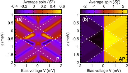
Figure 4: (color online) The average value of the $z$th component of the molecules’s total spin $\langle S_{t}^{z}\rangle$ for the parallel (a) and antiparallel (b) magnetic configurations. All parameters as in Fig. 2.

Spin-dependent transport through a SMM has a significant impact on its magnetic state. In Fig. 4 we show the average value of the molecule’s spin $z$th component in the stationary state, $\langle S_{t}^{z}\rangle$, calculated as a function of the bias voltage $V$ and energy of the LUMO level $\varepsilon$. In the antiparallel magnetic configuration, Fig. 4(b), the orientation of the molecule’s spin is straightforwardly related to the bias voltage, and for $V>0$ the spin is aligned along the easy axis $+z$, whereas for $V<0$ it is aligned along the $-z$ axis. Note, that in the regions corresponding to $Q=0$ and $Q=2$ the spin is equal to that of magnetic core, while for $Q=1$ it also includes the contribution from an electron in the LUMO level. By contrast, in the parallel configuration, Fig. 4(a), the value of $\langle S_{t}^{z}\rangle$ in the stationary state can be both positive and negative for each sign of the bias voltage, and it varies in a rather limited range close to zero. Moreover, $\langle S_{t}^{z}\rangle$ in the parallel (antiparallel) magnetic configuration is an even (odd) function of the bias voltage $V$.

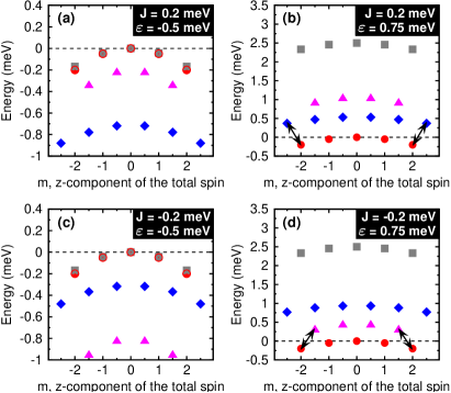
Figure 5: (color online) Energy spectrum of the molecule under consideration (relevant parameters given in the caption of Fig. 2) for $\varepsilon=-0.5$ meV (a,c) and $\varepsilon=0.75$ meV (b,d) in the case of ferromagnetic (a)-(b) and antiferromagnetic (c)-(d) coupling between the SMM’s core spin and the spin of electrons in the LUMO level. The dashed line represents the Fermi level of the leads when no external voltage bias is applied ($V=0$). Different sets of molecular states correspond to different values of the SMM’s total spin $S_{t}$, and/or the occupation number of the LUMO level: $|2;0,m\rangle$ ($\bullet$), $|5/2;1,m\rangle$ ($\blacklozenge$), $|3/2;1,m\rangle$ ($\blacktriangle$), and $|2;2,m\rangle$ ($\blacksquare$). Note that in (a) and (c) the degeneracy between states $|2;0,m\rangle$ and $|2;2,m\rangle$ takes place only for $m=0$.

To account for the transport properties in different regimes, especially of TMR and shot noise, in the following we present and discuss the gate and bias voltage dependence corresponding to various cross-sections of the relevant density plots mentioned above. More specifically, we will first consider transport properties in the linear response regime (Sec. IV.1), and then transport in the nonlinear regime (Sec. IV.2). In addition, whenever advisable and possible, we will also compare and relate our findings to existing results on quantum dot systems. At this point, it is however worth emphasizing that the problem of electron transport through a SMM is much more complex and physically richer than in the case of single quantum dots. Barnaś and Weymann (2008) This is because now the transfer of electrons occurs through many different many-body states of the coupled LUMO level and molecule’s magnetic core, see Eq. (II).

Since transport properties of a system are determined by its energy spectrum, it is instructive to analyze it in more detail. For molecules with only uniaxial anisotropy considered in this paper, the molecule’s Hamiltonian $\mathcal{H}_{\textrm{SMM}}$ can be diagonalized analytically (the relevant formulas can be found in Ref. [Misiorny and Barnaś, 2009a], from where the notation for molecular states has also been adopted). Energy spectrum of the molecule under consideration is presented in Fig. 5 for two different values of the LUMO level energy $\varepsilon$ and two values of the coupling parameter $J$. Each molecular state $|S_{t};n,m\rangle$ is labelled by the total spin number $S_{t}$, the occupation number $n$ of the LUMO level, and the eigenvalue $m$ of the $z$th component of the molecule’s total spin, $S_{t}^{z}\equiv S_{z}+\frac{1}{2}(c_{\uparrow}^{\dagger}c_{\uparrow}-c_{\downarrow}^{\dagger}c_{\downarrow})$, where the second term stands for the contribution from electrons in the LUMO level. The change of the LUMO level energy leads to the change in the energetic position of the spin-multiplets $|5/2;1,m\rangle$, $|3/2;1,m\rangle$ and $|2;2,m\rangle$ with respect to $|2;0,m\rangle$. The latter multiplet corresponds to uncharged molecule and therefore is independent of $\varepsilon$, see Fig. 5.

IV.1 Transport in the linear response regime

In this subsection we will focus on transport in the linear response regime. As we have already mentioned above, conductance in the linear response regime (see Fig. 2 for $V=0$), displays two resonance peaks separated approximately by $U$. For $J>0$ and $D(2S-1)\gg k_{\textrm{B}}T$, one can assume that the molecule is in the spin states of lowest energy. The position of the conductance peaks (resonances) corresponds then to $\varepsilon=\varepsilon_{01}$,

$$\varepsilon_{01}=\frac{JS}{2}+D_{1}S^{2}+\frac{g\mu_{\textrm{B}}|H_{z}|}{2},$$ (13)

for the transition from zero to single occupancy of the LUMO level, and to $\varepsilon=\varepsilon_{12}$,

$$\varepsilon_{12}=-\frac{JS}{2}-U+(D_{1}+D_{2})S^{2}-\frac{g\mu_{\textrm{B}}|H_{z}|}{2},$$ (14)

for the transition from single to double occupancy. It is worth noting that the above expressions may be useful for estimating the coupling constant $J$ from transport measurements. Moreover, from the above formulas one can conclude that the middle of the Coulomb blockade ($Q=1$ in Fig. 2) regime corresponds to $\varepsilon=\varepsilon_{m}$, with

$$\varepsilon_{m}=-\frac{U}{2}+\frac{2D_{1}+D_{2}}{2}S^{2}\,,$$ (15)

which for the parameters assumed in calculations gives $\varepsilon_{m}=-0.516$ meV. Interestingly, $\varepsilon_{m}$ is independent of the exchange coupling $J$, anisotropy constant $D$, and external magnetic field $H_{z}$, but it depends on the Coulomb interaction $U$, corrections $D_{1}$ and $D_{2}$ to the anisotropy due to finite occupation of the LUMO level, and the molecule’s spin number $S$. In fact, owing to finite constants $D_{1}$ and $D_{2}$, the particle-hole symmetry is broken, which manifests itself in an asymmetric behavior of transport properties, as will be shown below.

Figure 6(a) shows the total TMR in the linear response regime, where for comparison TMR in the sequential transport regime is also displayed (dash-dotted line). Clearly, the results obtained within the sequential tunneling approximation, which yield a constant TMR equal to $P^{2}/(1-P^{2})$, are not sufficient as the total (first plus second order) linear TMR displays a nontrivial dependence on the gate voltage. This behavior stems from the dependence of the second-order processes on the occupation number of the LUMO level.

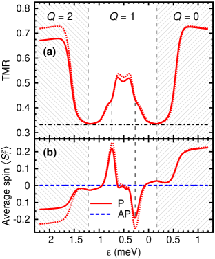
Figure 6: (color online) (a) TMR in the linear response regime for the parameters as in Fig. 2 (solid line). The dot-dashed line shows the TMR calculated in the first-order approximation. (b) Average value of the $z$th component of the molecule’s total spin in the (P) parallel (solid line) and (AP) antiparallel (dashed line) magnetic configurations. The dotted lines in (a) and (b) correspond to the case of $D_{1}=D_{2}=0$.

Generally, cotunneling processes can be divided into two groups with respect to whether or not the molecule remains in its initial state after a cotunneling process, Fig. 7(a)-(b). Although the cotunneling events do not change the charge state of the molecule, they can, however, modify its spin state (inelastic cotunneling). Moreover, the inelastic cotunneling processes can lead to magnetic switching of the molecule’s spin between two lowest energy states, as shown schematically in Fig. 7(b). We note that in addition to double-barrier cotunneling processes which transfer charge between two different electrodes, there are also single-barrier cotunneling processes, where an electron involved in the cotunneling process returns back to the same electrode. Although the latter processes do not contribute directly to the current flowing through the system, they can affect all the transport properties in an indirect way, by altering spin state of the molecule.

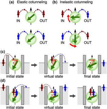
Figure 7: (color online) (a)-(b) Schematic representation of the elastic and inelastic electron cotunneling processes. The two bottom panels show examples of inelastic cotunneling processes leading to increase of the $z$th component of the SMM’s spin in the situation when the LUMO level is: (c) empty ($Q=0$) and (d) doubly occupied ($Q=2$). Note that $V\to 0$ in the linear response regime, so we assume $\mu_{L}=\mu_{R}+0^{+}$. When in the ground state the molecule is occupied by a single electron, $Q=1$, inelastic processes can generally occur via two virtual states associated with empty and doubly occupied LUMO level.

IV.1.1 Cotunneling regime with empty and doubly occupied LUMO level

When the LUMO level is either empty ($Q=0$) or fully occupied ($Q=2$), the total TMR in the corresponding cotunneling regions is slightly larger than the Julliere value, Julliere (1975) ${\rm TMR^{Jull.}}=2P^{2}/(1-P^{2})$ (${\rm TMR^{Jull.}}=2/3$ for $P=0.5$), see Fig. 6(a). Electron transport in these regions is primarily due to elastic cotunneling processes which change neither the electron spin in the LUMO level nor the spin of molecule’s core, and thus are fully coherent. An example of such process is sketched in Fig. 7(a). The enhancement of TMR above the Julliere value is then associated with the exchange coupling of the LUMO level to the molecule’s core spin, which additionally admits inelastic cotunneling processes in these regions. In addition, the enhanced TMR may also result from the fact that by using the crossover perturbation scheme, Weymann et al. (2005) we also include some effects associated with third-order processes, which may further increase the TMR. Moreover, unlike the case of a single quantum dot, Barnaś and Weymann (2008); Weymann et al. (2005) the maximal values of TMR reached for $Q=0$ and $Q=2$ do not necessarily have to be equal, see Fig. 6(a). Below, we discuss these new features in more details.

From the energy spectrum displayed in Fig. 5(b) follows that the dominant elastic transfer of electrons between the leads for $Q=0$ takes place via the following virtual transitions: $|2;0,-2\rangle\leftrightarrow|5/2;1,-5/2\rangle$ and $|2;0,2\rangle\leftrightarrow|5/2;1,5/2\rangle$ [indicated with black arrows in Fig. 5(b)]. In the parallel configuration, the former transitions establish the transport channel for minority electrons, whereas the latter ones for majority electrons. The asymmetry between the occupation probabilities of the states $|2;0,-2\rangle$ and $|2;0,2\rangle$ (with $|2;0,2\rangle$ being favored), which occurs due to inelastic cotunneling processes, gives rise to increased transport of majority electrons. On the other hand, there is no such asymmetry in the antiparallel configuration. This, in turn, leads to an enhancement of the TMR above the Julliere value, Fig. 6(a).

Similar arguments also hold for the case of $Q=2$, where the molecular states $|2;2,m\rangle$ correspond to double occupancy of the LUMO level. The main difference as compared to the situation discussed above is that now in a cotunneling process the electron first has to tunnel out of the LUMO level and then another electron can tunnel onto the molecule [Fig. 7(d)]. Analysis similar to that for $Q=0$ shows that in the parallel configuration the inelastic cotunneling processes result in lowering of the $z$th component of the SMM’s spin, see Fig. 6(b). Moreover, the asymmetry between the occupation probabilities of the states $|2;2,-2\rangle$ and $|2;2,2\rangle$, where now $|2;2,-2\rangle$ is favored, leads to increased elastic cotunneling of spin majority electrons and therefore gives rise to enhanced TMR for $Q=2$.

Another interesting feature of TMR in the linear response regime, shown in Fig. 6(a), is the difference in its magnitude in the cotunneling regions corresponding to $Q=0$ and $Q=2$. This is contrary to the case of Anderson model, where the linear TMR was found to be symmetric with respect to the particle-hole symmetry point, $\varepsilon=-U/2$. Weymann et al. (2005) In the case considered here, the situation is different due to coupling of the LUMO level to the molecule’s spin, and also due to occupation dependent corrections to the anisotropy constant, see Eq. (II). These corrections reduce the uniaxial anisotropy of the molecule with increasing number of electrons in the LUMO level. As a result, the height of the energy barrier between the two lowest molecular spin states is also diminished for $Q=1$ and $Q=2$, and so are the energy gaps between neighboring molecular states within the relevant spin multiplets. For this reason, the probability distribution of the molecular states for $Q=2$ (and also for $Q=1$) is more uniform than for $Q=0$, see the solid line in Fig. 6(b). Consequently, the value of TMR for $Q=2$ is smaller than for $Q=0$. Thus, the observed asymmetry with respect to $\varepsilon=\varepsilon_{m}$ is due to the lack of particle-hole symmetry in the system when $D_{1}$ and $D_{2}$ are nonzero. However, if the influence of the LUMO level’s occupation on the anisotropy were negligible, $D_{1}\approx D_{2}\approx 0$ (the states $|2;0,m\rangle$ and $|2;2,m\rangle$ in Fig. 5(a) were then degenerate for every $m$), the symmetry with respect to $\varepsilon=\varepsilon_{m}=-U/2$ would be restored. This situation is presented by the dotted curves in Fig. 6, which clearly show that the asymmetric behavior of TMR and $\langle S_{t}^{z}\rangle$ is related to the corrections to anisotropy constants and the lack of particle-hole symmetry.

IV.1.2 Cotunneling regime with singly occupied LUMO level

Interestingly, in the Coulomb blockade regime, with one electron in the LUMO level ($Q=1$), the TMR reaches local maxima close to the center of the Coulomb gap, and a shallow local minimum just in the middle, i.e. for $\varepsilon=\varepsilon_{m}$. This behavior is different from that observed in single-level quantum dots, where linear TMR in the Coulomb blockade regime becomes suppressed and reaches a global minimum when $\varepsilon=-U/2$. Weymann et al. (2005) As in the case of $Q=0$ and $Q=2$ discussed above, the origin of increased TMR for $Q=1$ can be generally assigned to the modification of the probability distribution of molecular states due to inelastic cotunneling processes, Fig. 7(b). In turn, the appearance of the local minimum in the center of the $Q=1$ region is related to the fact that when $\varepsilon=\varepsilon_{m}$, the virtual states for leading inelastic cotunneling processes, which belong to spin multiplets $|2;0,m\rangle$ and $|2;2,m\rangle$, become pairwise degenerate (in the present situation, $|2;0,\pm 2\rangle$ with $|2;2,\pm 2\rangle$). This means that in the parallel configuration cotunneling processes involving empty and doubly occupied virtual states occur at equal rates. As a consequence, the average spin on the molecule tends to zero, see Fig. 6(b), and TMR displays a local minimum for $\varepsilon=\varepsilon_{m}$.

IV.1.3 Resonant tunneling regime

For resonant energies, Eqs. (13)-(14), where the occupancy $Q$ of the molecule changes, the sequential tunneling processes play a dominant role. This results in the reduction of TMR to approximately half of the Julliere value, Julliere (1975) see the boundaries between the hatched and non-hatched areas in Fig. 6. The rate of first-order tunneling processes increases whenever the two neighboring charge states of the molecule become degenerate, provided that the conditions $|\Delta n|=1$ and $|\Delta S_{t}^{z}|=1/2$ are simultaneously satisfied, where $|\Delta n|$ and $|\Delta S_{t}^{z}|$ describe change in the occupation and spin of the molecule. This means that for $\varepsilon=\varepsilon_{01}\approx 0.18$ meV the degeneration between the empty and singly occupied states, $|2;0;\pm 2\rangle$ and $|5/2;1,\pm 5/2\rangle$, is observed, whereas for $\varepsilon=\varepsilon_{12}\approx-1.21$ meV the states with a single and two electrons on the LUMO level, $|5/2;1,\pm 5/2\rangle$ and $|2;2;\pm 2\rangle$, are degenerate. Moreover, we also note that for $\Gamma\approx k_{B}T$, TMR can be reduced further due to increased role of second-order processes giving rise to the renormalization of the LUMO level. Weymann et al. (2005)

IV.2 Transport in the nonlinear response regime

The influence of sequential tunneling on transport characteristics, as well as on magnetic state of the SMM, grows with increasing bias voltage. For voltages above the threshold for sequential tunneling, first-order processes determine transport and the influence of cotunneling is rather small. However, when applied voltage is below the threshold, sequential tunneling becomes exponentially suppressed and second-order processes give the dominant contribution to the current, and need to be taken into account to get a proper physical picture. Figure 8 shows the bias dependence of the current, differential conductance, TMR and Fano factor, calculated for $\varepsilon=-0.5$ meV and $\varepsilon=0.75$ meV. The former case corresponds to the situation where the LUMO level in equilibrium is singly occupied, Fig. 5(a), while in the latter case it is empty, Fig. 5(b). One can see that cotunneling significantly modifies the first-order results in the blockade regimes and this modification is most pronounced for TMR and shot noise.

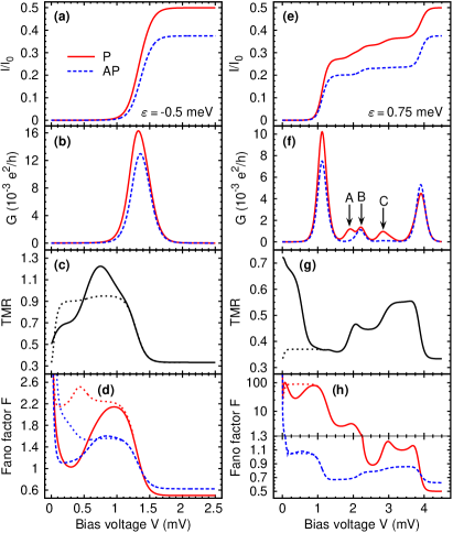
Figure 8: (color online) Bias dependence of the current (a,e), differential conductance (b,f), Fano factor (d,h) in the parallel (solid lines) and antiparallel (dashed lines) configurations and TMR (c,g) for $\varepsilon=-0.5$ meV (a)-(d) and $\varepsilon=0.75$ meV (e)-(h). The parameters are the same as in Fig. 2, and $I_{0}=e\Gamma/\hbar\approx 0.5$ nA. The dotted lines show the results obtained taking into account only first-order tunneling processes. The effect of cotunneling is most pronounced in the TMR and Fano factor.

IV.2.1 Transport characteristics in the case of $\varepsilon_{01}>\varepsilon>\varepsilon_{12}$

Consider first the case when in equilibrium the LUMO level is singly occupied (left panel of Fig. 8). At low temperatures and low voltages, the molecule with almost equal probabilities is in one of the two ground states $|5/2;1,\pm 5/2\rangle$, Fig. 5(a). When a small bias voltage is applied, some current flows due to cotunneling processes through virtual states of the system. If the bias voltage exceeds threshold for sequential tunneling, the current significantly increases and becomes dominated by first-order processes, when electrons tunnel one-by-one through the molecule.

Since elastic cotunneling in the antiparallel configuration occurs essentially through the minority-majority and majority-minority channels, whereas for parallel alignment through the majority-majority and minority-minority ones, one observes growth of TMR with increasing bias voltage, which reaches a local maximum just before the threshold for sequential tunneling. This is associated with nonequilibrium spin accumulation in the LUMO level for the antiparallel configuration, which leads to suppression of charge transport and thus to enhanced TMR. Further increase of transport voltage results in a decrease of TMR to approximately 1/3 (for $P_{L}=P_{R}=0.5$), which is typical of the sequential tunneling regime, when all molecular states actively participate in transport. Barnaś and Weymann (2008); Weymann et al. (2005) In the parallel magnetic configuration all states are then equally populated, so that average magnetic moment of the molecule vanishes, $\langle S_{t}^{z}\rangle$=0. This differs from the antiparallel case, in which only the states with large positive $z$th component of the SMM’s spin have remarkable probabilities. Finally, we note that the slight shift between the peaks in differential conductance corresponding to different magnetic configurations, see Fig. 8(b), is a consequence of nonequilibrium spin accumulation in the LUMO level in the antiparallel configuration. Similar behavior has been observed in the case of transport through ferromagnetic single-electron transistors. Weymann and Barnaś (2006)

The Fano factor in the parallel ($F_{\textrm{P}}$) and antiparallel ($F_{\textrm{AP}}$) configurations is shown in Fig. 8(d). For low bias voltages, the shot noise is determined by thermal Johnson-Nyquist noise, which results in a divergency of the Fano factor for $V\to 0$ (current tends to zero). When a finite bias voltage is applied to the system, the Fano factor in both magnetic configurations drops to the value close to unity, which indicates that transport occurs mainly due to elastic cotunneling processes. Such processes are stochastic and uncorrelated in time, so the shot noise is Poissonian. When bias voltage increases further, the shot noise is enhanced due to bunching of inelastic cotunneling processes and reaches maximum just before threshold for sequential tunneling. At the threshold voltage, sequential tunneling processes begin to dominate transport and the noise becomes sub-Poissonian. This indicates that tunneling processes in the sequential tunneling regime are correlated due to Coulomb correlation and Pauli principle, which generally gives rise to suppressed shot noise as compared to the Poissonian value. Furthermore, another feature clearly visible in the Coulomb blockade regime is the difference in Fano factors for parallel and antiparallel magnetic configurations. More specifically, shot noise in the parallel configuration is larger than in the antiparallel one. This behavior is associated with the fact that transport in the parallel configuration occurs mainly through two competing majority-majority and minority-minority spin channels, which in turn increases fluctuations, thus $F_{\textrm{P}}>F_{\textrm{AP}}$.

IV.2.2 Transport characteristics in the case of $\varepsilon>\varepsilon_{01}$

Let us consider now the situation shown in the right panel of Fig. 8, i.e. when the LUMO level of the molecule is empty at equilibrium, Fig. 5(b). The initial large value of TMR, whose origin was discussed above, drops sharply as the bias voltage approaches the threshold value for sequential transport. In turn, the first pronounced peak in differential conductance appears when the following transitions become allowed: $|2;0,\pm 2\rangle\leftrightarrow|5/2;1,\pm 5/2\rangle$ [denoted by arrows is Fig. 5(b)]. It is important to note that, when a spin-multiplet enters the transport energy window, the first states that take part in transport are those with the largest $|\langle S_{t}^{z}\rangle|$ (lowest energy). Consequently, in the parallel magnetic configuration the system can be temporarily trapped in some molecular spin states of lower energy. For larger bias voltage, additional small peaks appear in the conductance for parallel configuration, and some of them are also visible in the antiparallel configuration. In general, these peaks are related to transitions involving states from the multiplet $|3/2;1,m\rangle$: $|2;0,\pm 1\rangle\leftrightarrow|3/2;1,\pm 3/2\rangle$ (A), $|2;0,\pm 2\rangle\leftrightarrow|3/2;1,\pm 3/2\rangle$ (B) and $|3/2;1,\pm 3/2\rangle\leftrightarrow|2;2,\pm 2\rangle$ (C), respectively, see Fig. 8(f). In the parallel configuration all the three peaks are visible, whereas for antiparallel alignment only the peak B can be clearly resolved. Since in the antiparallel configuration tunneling processes tend to increase the $z$th component of the SMM’s total spin, the probability of finding the molecule in any of the spin states $|2;0,m\rangle$ differs significantly from zero only for $m=2$. As a consequence, in the antiparallel configuration most favorable transitions are those having the initial state $|2;0,2\rangle$, and thus the peaks A and C are suppressed, see Fig. 8(f).

Furthermore, as soon as all states within a certain spin-multiplet become energetically accessible, the probability of finding the molecule in each of these states becomes roughly equal. On the other hand, in the antiparallel configuration the system tends towards maximum value (for $V>0$) of the $z$th component of SMM’s spin. For these reasons, some regions of the increased TMR are present in Fig. 8(g).

The corresponding Fano factor is shown in Fig. 8(h). At low bias, the Fano factor drops with increasing voltage. However, its bias dependence is distinctively different in both magnetic configurations. In the antiparallel configuration, the Fano factor tends to unity, indicating that transport is due to uncorrelated tunneling events. In the parallel configuration, on the other hand, we observe large super-Poissonian shot noise. The increased current fluctuations result mainly from the interplay between different cotunneling processes and bunching of inelastic cotunneling. In addition, as mentioned previously, in the parallel configuration the molecule can be temporarily trapped in some molecular spin states of lower energy, which also gives rise to super-Poissonian shot noise. When the bias voltage is increased above the threshold for sequential tunneling, the Fano factor becomes suppressed and the shot noise is generally sub-Poissonian. Finally, we also note that super-Poissonian shot noise in the cotunneling regime has already been observed in quantum dots and carbon nanotubes, Cottet et al. (2004); Onac et al. (2006); Zhang et al. (2007); Barnaś and Weymann (2008) where the increased noise was associated with bunching of inelastic spin-flip cotunneling events.

IV.3 Dependence on exchange coupling strength

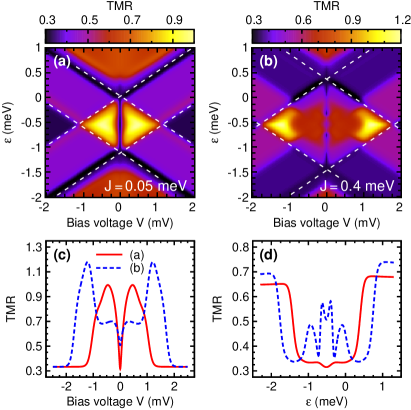
Figure 9: (color online) Density plot of TMR for $J=0.05$ meV (a) and $J=0.4$ meV (b). The bottom panels display cross-sections of (a) and (b) for the constant energy of the molecule’s LUMO level $\varepsilon=-0.5$ meV (c) and the constant bias voltage $V=0$ mV (d). Other parameters are the same as in Fig. 2.

Tunnel magnetoresistance may become significantly changed by altering the strength of ferromagnetic exchange coupling between the LUMO level and the SMM’s core spin, as shown in Fig. 9. With decreasing $J$, the energy separation between the relevant molecule states corresponding to the single occupancy of the LUMO level is also diminished (slanted squares and triangles in Fig. 5 start then approaching each other). This, in turn, leads to a reduction in size of the central diamond-shaped region, representing transport in the Coulomb blockade regime through the molecule with one electron in the LUMO level. As follows from Fig. 9(a), behavior of TMR for small values of $J$ starts bearing some resemblance to that of a single-level quantum dot. Barnaś and Weymann (2008); Weymann et al. (2005) Furthermore, in the linear response regime, Fig. 9(d), the enhanced TMR around the electron-hole symmetry point is no longer visible, and instead a global minimum develops there. In fact, in the limit of $J=0$ one observes a simple quantum-dot-like transport behavior. Weymann et al. (2005); Barnaś and Weymann (2008)

In the opposite limit of large $J$ shown in Fig. 9(b), the maxima in the total linear TMR are shifted away from the zero bias point. This is a consequence of increased energy gaps between the ground states $|5/2;1,\pm 5/2\rangle$ and the nearest lying states satisfying $|\Delta n|=1$ and $|\Delta S_{t}^{z}|=1/2$, i.e. $|2;0(2),\pm 2\rangle$. Another interesting feature of TMR visible in the linear response regime is the presence of additional two local minima around $\varepsilon=\varepsilon_{m}$, see Fig. 9(d). Some precursors of these minima can be actually seen also in Fig. 6(a) as two steep steps on both sides of the plot’s central part. Generally, they stem from an uneven probability distribution of the molecular spin states with positive and negative $z$th component of the SMM’s spin in the parallel magnetic configuration, see Fig. 6(b). This in turn means that elastic cotunneling processes occur mainly through the minority-minority spin channel, so that transport is effectively suppressed. In the present situation, the minima are more distinct due to larger energy separation between the spin-multiplets $|5/2;1,m\rangle$ and $|3/2;1,m\rangle$.

In the nonlinear response regime, on the other hand, the TMR exhibits a minimum at zero bias and starts increasing with the bias voltage to reach a maximum around the threshold for sequential tunneling. This is associated with nonequilibrium spin accumulation in the LUMO level, which is present in the antiparallel configuration. We note that although the magnitude and position of the TMR maxima in the nonlinear response regime of the Coulomb blockade depend significantly on the exchange constant $J$, the general qualitative behavior of TMR is rather independent of $J$, see Figs. 9(c) and 8(c).

IV.4 Transport in the presence of a longitudinal external magnetic field

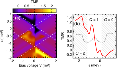
Figure 10: (color online) (a) Density plot of TMR in the case when the external magnetic field $H_{z}=0.216$ T ($g\mu_{\textrm{B}}H_{z}=0.025$ meV) is applied along the easy axis of the molecule. (b) TMR in the linear response regime (solid line). For comparison, TMR in the absence of external magnetic field (dotted line in (b)) is also shown. The other parameters are the same as in Fig. 2.

Let us consider now the main effects due to a finite magnetic field applied to the system. When the field is along the easy axis of the molecule, its effects occur via modification of the energy of molecular spin states. On the other hand, when the field possesses also a transversal component, it leads to symmetry-breaking effects and the $z$th component of the SMM’s total spin is no more a good quantum number. Timm (2007) If the magnetic field is additionally time-dependent, one can expect the phenomenon of quantum tunneling of magnetization to occur. Chudnovsky and Tejada (1998); Gatteschi and Sessoli (2003); Misiorny and Barnaś (2009a) Since the primary focus of the present paper is on transport through SMMs with uniaxial anisotropy, in the following we consider only a longitudinal magnetic field.

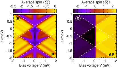
Figure 11: (color online) Average value of the $z$th component of the total molecule’s spin in the parallel (a) and antiparallel (b) magnetic configurations, when an external field $H_{z}=0.216$ T is applied along the $z$-axis. The other parameters are the same as in Fig. 2.

Figure 10(a) shows the density plot of TMR for a magnetic field applied along the easy axis of a SMM. Despite rather modest value of the field (for comparison, in the experiment on the $\textrm{Mn}_{12}$ molecule attached to nonmagnetic metallic electrodes by Jo et al., the field of 8 T was used, Ref. [Jo et al., 2006]), a drastic change in transport properties of the system is observed [contrast Fig. 10(a) with Fig. 3(a)]. First, the field breaks the symmetry with respect to the bias reversal. Second, it admits the situation when conductance in the antiparallel magnetic configuration is larger than in the parallel one (black regions corresponding to negative TMR). Furthermore, in the parallel configuration the average spin $\langle S_{t}^{z}\rangle$ in the Coulomb blockade region can take large negative values, while in the absence of magnetic field the SMM’s spin prefers orientation in the plane normal to the easy axis. This implies that for parallel alignment of leads’ magnetizations, the molecule’s spin tends to align antiparallel to the $z$-axis, Fig. 11(a). However, when the sequential tunneling processes are allowed, this tendency is generally reduced. In the antiparallel configuration, on the other hand, the behavior of the average molecule’s spin is similar to that for $H_{z}=0$, see Figs. 11(b) and 4(b).

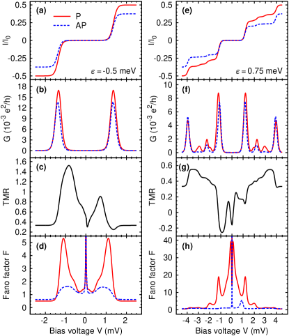
Figure 12: (online color) The current (a,e), differential conductance (b,f), Fano factor (d,h) in the parallel (solid lines) and antiparallel (dashed lines) configurations, and the TMR (c,g) for $\varepsilon=-0.5$ meV (a)-(d) and $\varepsilon=0.75$ meV (e)-(h) as a function of the bias voltage. An external magnetic field $H_{z}=0.216$ T is applied along the $z$-axis, while the other parameters are the same as in Fig. 2.

In the linear response regime, a large change of TMR is observed when $\varepsilon$ is comparable to $\varepsilon_{m}$, i.e. in the middle of the Coulomb blockade regime, see Fig. 10(b). This stems from the fact that at this point the dominating spin-dependent channel for transport due to cotunneling processes in the parallel magnetic configuration switches from the minority-minority channel (for $\varepsilon>\varepsilon_{m}$) to majority-majority one (for $\varepsilon<\varepsilon_{m}$). In the antiparallel configuration, on the other hand, the dominant channel is rather associated with majority-minority spin bands, irrespective of the position of the LUMO level. As a consequence, for $\varepsilon>\varepsilon_{m}$ the current in the parallel configuration is smaller than that in the antiparallel one, leading to negative TMR, whereas for $\varepsilon<\varepsilon_{m}$ the situation is opposite and one finds a large positive TMR effect, see Fig. 10(b).

The transport characteristics in the nonlinear response regime, and in the presence of external magnetic field, are shown in Fig. 12, where the left (right) panel corresponds to the situation where in the ground state the molecule is singly occupied (empty). The asymmetry with respect to the bias reversal is clearly visible, especially in the tunnel magnetoresistance, see Fig. 12(c) and (g). Interestingly, this asymmetric behavior is mainly observed in the cotunneling regime, as can be also seen in Fig. 10(a). This results from the fact that the degeneracy of the molecule’s ground state is removed for $H_{z}\neq 0$ and the SMM becomes polarized. In turn, transport in the cotunneling regime depends mainly on the system’s ground state, which is the initial state for the cotunneling processes. As a consequence, in the parallel configuration the current is always mediated by electrons belonging to the same spin bands of the leads, whereas in the antiparallel configuration, the dominant transport channel is associated either with majority or minority electrons, depending on the direction of the current flow. Thus, the current in the antiparallel configuration becomes in general asymmetric with respect to the bias reversal, which gives rise to the associated asymmetric behavior of TMR.

For voltages larger than the splitting due to the Zeeman term ($g\mu_{\textrm{B}}H_{z}=0.025$ meV), the inelastic cotunneling processes start taking part in transport. The competition between the elastic and inelastic cotunneling leads in turn to large super-Poissonian shot noise, which in the parallel configuration is enhanced due to additional fluctuations associated with cotunneling through majority-majority and minority-minority spin channels, see Fig. 12(d) and (h). On the other hand, when the voltage exceeds threshold for sequential tunneling, more states take part in transport and the asymmetry with respect to the bias reversal is suppressed. The same tendency is observed in the shot noise, which in the sequential tunneling regime becomes generally sub-Poissonian.

IV.5 Antiferromagnetic coupling between the LUMO level and SMM’s core spin

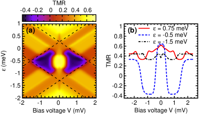
Figure 13: (color online) (a) The total tunnel magnetoresistance in the case of antiferromagnetic coupling between the SMM’s core spin and the spin in the LUMO level, calculated for $J=-0.2$ meV and other parameters as in Fig. 2. (b) Representative cross-sections of the density plot in (a) for several values of the LUMO level energy $\varepsilon$.

The numerical results presented up to now concerned the case of ferromagnetic coupling ($J>0$) between the LUMO level and the SMM’s core spin. However, since the type of such an interaction generally depends on the SMM’s internal structure, the exchange coupling can be also of antiferromagnetic type ($J<0$). In this subsection we discuss how the main transport properties of the system change when the exchange coupling becomes antiferromagnetic.

First of all, we note that in the case of antiferromagnetic coupling between the LUMO level and molecule’s core spin the formulas estimating the position of conductance resonances need some modification. Equations (13)-(14) were derived assuming the degeneracy between the states $|2;0,\pm 2\rangle$ ($|5/2;1,\pm 5/2\rangle$) and $|5/2;1,\pm 5/2\rangle$ ($|2;2,\pm 2\rangle$). For $J<0$, however, the condition has to be modified by changing $|5/2;1,\pm 5/2\rangle$ into $|3/2;1,\pm 3/2\rangle$, where the upper signs apply for $H_{z}<0$, and the lower ones for $H_{z}>0$. The relevant equations take now the following form:

$$\varepsilon_{01}=\frac{|J|}{4}+D_{1}S^{2}-\Delta\varepsilon$$ (16)

for the transition from empty to singly occupied states, and

$$\varepsilon_{12}=-\frac{|J|}{4}-U+(D_{1}+D_{2})S^{2}+\Delta\varepsilon$$ (17)

for the transition between singly and doubly occupied states, where

$$\Delta\varepsilon =D^{(1)}\frac{2S-1}{2}+\frac{g\mu_{\textrm{B}}|H_{z}|}{2}$$

$$-\sqrt{D^{(1)}(D^{(1)}+|J|)\frac{(2S-1)^{2}}{4}+\frac{J^{2}}{16}(2S+1)^{2}},$$ (18)

with $D^{(1)}=D+D_{1}$.

The most apparent new feature of the total TMR for $J<0$, as shown in Fig. 13(a), is its negative value in the Coulomb blockade regime ($Q=1$). The negative TMR occurs in transport regimes where the maximum of TMR was observed for $J>0$, i.e. close to the threshold for sequential tunneling, see Fig. 3(a). Such behavior of TMR originates from the fact that now spin-multiplets $|5/2;1,m\rangle$ and $|3/2;1,m\rangle$ exchange their positions, Fig. 5(c)-(d), so that the multiplet corresponding to smaller total spin of the molecule for antiferromagnetic coupling corresponds to lower energy. Consequently, in the Coulomb blockade the current flowing in the antiparallel configuration is larger than that in the parallel configuration, which gives rise to the negative TMR effect.

The linear response TMR is shown in Fig. 14(a). Unlike the case of ferromagnetic coupling, the values of TMR for $Q=0$ and $Q=2$ are smaller as compared to those in the case of transport through single-level quantum dots. Barnaś and Weymann (2008); Weymann et al. (2005) On the other hand, for $Q=1$ the TMR can take values exceeding those found in the case of ferromagnetic exchange coupling. For $\varepsilon>\varepsilon_{01}$, the equilibrium probability distribution of different molecular spin states $|2;0,m\rangle$ becomes changed owing to inelastic cotunneling processes, similarly as described in Sec. IV.1. The key difference with respect to $J>0$ is that now dominating elastic cotunneling transitions for $Q=0$ are those with initial states $|2;0,\pm 2\rangle$ and virtual states $|3/2;1,\pm 3/2\rangle$ [indicated by black arrows in Fig. 5(d)].

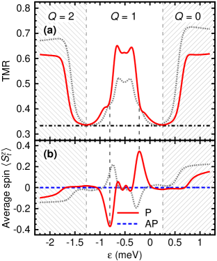
Figure 14: (color online) Tunnel magnetoresistance (a) and the $z$th component of the molecule’s total spin (b) calculated in the linear response regime for the antiferromagnetic coupling of the SMM’s core spin with the spin of the LUMO level ($J=-0.2$ meV and other parameters as in Fig. 2). Dotted lines show the results obtained for the case of ferromagnetic exchange coupling, see Fig. 6 – in (b) the dotted line corresponds to the parallel configuration.

V Summary and conclusions

We have systematically analyzed the transport properties of a single-molecule magnet coupled to ferromagnetic leads in both sequential and cotunneling regimes. The transport processes in such a system occur due to tunneling through the LUMO level which is exchange coupled to the molecule’s core spin. By employing the real-time diagrammatic technique, we have calculated the current, tunnel magnetoresistance and shot noise in both the linear and nonlinear response regimes. The results show that the inclusion of second-order processes is crucial for a proper description of transport characteristics.

Assuming the ferromagnetic coupling between the LUMO level and the molecule’s core spin, we have shown that TMR in the Coulomb blockade regime can be enhanced above the Julliere value. This enhancement is associated with nonequilibrium spin accumulation in the molecule. Moreover, we have found an asymmetric behavior of the linear response TMR with respect to the middle of the Coulomb blockade regime, and its strong dependence on the number of electrons in the LUMO level. The asymmetry is associated with corrections to anisotropy constant due to a nonzero occupation of the molecule, which breaks the particle-hole symmetry in the system. In addition, we have shown that the competition between the elastic and inelastic second-order processes leads to large super-Poissonian shot noise. The shot noise is further enhanced in the parallel configuration due to additional fluctuations associated with majority-majority and minority-minority spin channels for electronic transport. On the other hand, for bias voltages above the threshold for sequential tunneling, the shot noise becomes generally sub-Poissonian, indicating the role of correlations in sequential transport.

We have also discussed how transport properties depend on the strength of the exchange coupling $J$ between the LUMO level and the molecule’s core spin. When the exchange coupling is relatively weak, the transport behavior of the system resembles that of single-level quantum dots, whereas with increasing exchange constant, the transport characteristics change in a nontrivial way and become distinctively different from those of quantum dots. In addition, it turned out that the position of maxima of TMR in the Coulomb blockade depend linearly on the strength of the exchange coupling. This may be useful in determining the magnitude of exchange constant experimentally.

Furthermore, we have studied the effects of external magnetic field and shown that current flowing through the SMM becomes then asymmetric with respect to the bias reversal. We have found a strong dependence of TMR on the number of electrons occupying the LUMO level. When the LUMO level is empty, the TMR may become negative, while for doubly occupied LUMO level tunnel magnetoresistance is much enhanced. Finally, we have also discussed how transport properties change when the coupling between the LUMO level and molecule’s core becomes antiferromagnetic. In that case we predict a large negative TMR effect in the Coulomb blockade regime, exactly where for ferromagnetic coupling an enhanced TMR was observed. Thus, the sign of TMR may provide an information on the type of exchange interaction, which may be of assistance for future experiments.

To conclude, we note that although the numerical results presented in this paper concern SMMs coupled to ferromagnetic leads, most of the qualitative results are applicable also to SMMs coupled to nonmagnetic electrodes. Apart from this, we note that the model we have studied also corresponds to systems consisting of a single-level quantum dot exchange-coupled to a spin $S$. In fact, very recently a similar device built of a quantum dot coupled through spin exchange interaction to metallic island have been implemented to experimentally access the quantum critical point between the Fermi liquid and non-Fermi liquid regimes. Potok et al. (2007)