Gas lasers with wave-chaotic resonators

Abstract

Semiclassical multimode laser theory is extended to gas lasers with open two-dimensional resonators of arbitrary shape. The Doppler frequency shift of the linear-gain coefficient leads to an additional linear coupling between the modes, which, however, is shown to be negligible. The nonlinear laser equations simplify in the special case of wave-chaotic resonators. In the single-mode regime, the intensity of a chaotic laser, as a function of the mode frequency, displays a local minimum at the frequency of the atomic transition. The width of the minimum scales with the inhomogeneous linewidth, in contrast to the Lamb dip in uniaxial resonators whose width is given by the homogeneous linewidth.

1 Introduction

Theory of gas lasers was developed some decades ago and is well covered in the literature [1, 2]. The gas lasers are characterized by their capability to emit light at frequencies that differ from the atomic-transition frequency by more than a homogeneous linewidth. This property is a consequence of the coherent amplification by moving atoms that interact with the electric field at Doppler-shifted frequencies. If a resonance frequency of the cavity is continuously changed, the intensity of the single mode drops within the homogeneous linewidth of the atomic frequency. This narrow local minimum in the inhomogeneously broadened line, the Lamb dip [3], can be observed in uniaxial cavities that support standing waves. The Lamb dip has been utilized for stabilization of laser frequency [4] and precise detection of atomic-transition frequency and line shape (Lamb-dip spectroscopy) [5].

The theory of lasers (including gas lasers) was originally intended for low-loss resonators with a well-defined direction of propagation. The continuing interest in random [6, 7] and chaotic [8] lasers has motivated extensions of the conventional theory to irregular and strongly open systems [8, 9, 10, 11, 12, 13]. These improvements relate to a number of aspects, such as construction of a quasimode basis of the open cavity, description of linear and nonlinear coupling between the lasing modes in irregular lasers, and incorporating the statistics of eigenfrequencies and eigenfunctions in the laser equations (see Ref. [14] for a review).

In the present article, the semiclassical theory of gas lasers is generalized to lasers with open two-dimensional resonators of arbitrary shape. Equations for the amplitudes and frequencies of lasing modes are derived by expanding the atomic polarization in the powers of electric field and keeping the linear and third-order contributions. Since the dependence of the linear gain on the frequency is modified by the Doppler shifts in the frames of moving atoms, there exists an additional linear coupling between the modes. This effect is similar to the gain-induced coupling in systems with spatially inhomogeneous refractive index [11] or pumping [14]. We can argue, however, that the the magnitude of the coupling in gas lasers is negligible under reasonable assumptions. The nonlinear terms in the laser equations simplify for the weakly open cavities of chaotic geometry, where the eigenmodes can be modeled by a superposition of plane waves propagating in random directions [15, 16]. In this system, the intensity of a single lasing mode, as a function of its frequency, has a local minimum at the frequency of the atomic transition. In contrast to the Lamb dip in uniaxial resonators, the width of the minimum is comparable to the inhomogeneous linewidth.

2 Semiclassical theory of gas lasers

2.1 Semiclassical laser equations

We consider an open resonator of arbitrary shape, which, in general, can be filled with a homogeneous inactive medium characterized by a real dielectric constant $\epsilon$. The lasing action is provided by active atoms located inside the resonator. In the simplest model, only the the two atomic levels responsible for the lasing transition are described dynamically, whereas the information about the remaining degrees of freedom is contained in the empirical parameters: the homogeneous atomic linewidth $\gamma_{\perp}$, the population-inversion decay rate $\gamma_{\parallel}$, and the unsaturated population difference (per unit volume) $\Delta n_{0}$. Then the system of atoms can be characterized by the polarization $\mathbf{P}(\mathbf{r},t)$ and the population-inversion density (the difference between the populations of the upper and lower levels per volume) $\Delta n(\mathbf{r},t)$. The interaction of these quantities and the classical electric field $\mathbf{E}(\mathbf{r},t)$ in the resonator is specified by the semiclassical laser equations [2]

$$\frac{\epsilon}{c^{2}}\frac{\partial^{2}\mathbf{E}}{\partial t^{2}}+\nabla\times(\nabla\times\mathbf{E})=-\frac{4\pi}{c^{2}}\frac{\partial^{2}}{\partial t^{2}}\mathbf{P}(\mathbf{r},t),$$ (1)

$$\left(\frac{\partial^{2}}{\partial t^{2}}+2\gamma_{\perp}\frac{\partial}{\partial t}+\nu^{2}\right)\mathbf{P}=-2\nu\frac{d^{2}}{\hbar}\mathbf{E}(\mathbf{r},t)\,\Delta n(\mathbf{r},t),$$ (2)

$$\frac{\partial\Delta n}{\partial t}-\gamma_{\parallel}(\Delta n_{0}-\Delta n)=\frac{2}{\hbar\nu}\mathbf{E}(\mathbf{r},t)\cdot\frac{\partial\mathbf{P}(\mathbf{r},t)}{\partial t},$$ (3)

where $\nu$ is the atomic-transition frequency and $d$ is the atomic dipole matrix element. The first equation follows from the Maxwell equations (written in the Gaussian units) and has the form of a wave equation with the polarization as a source. The second equation describes the dipole interaction with the field and the decay of polarization due to stochastic degrees of freedom. The third equation describes the energy exchange between the atoms and the field, as well as the relaxation of the population inversion. If the field were absent, $\Delta n(\mathbf{r},t)$ would reach the stationary value of $\Delta n_{0}$. We will use this parameter as a measure of the pump strength.

In the gas laser, the active atoms are moving with constant velocities $\mathbf{v}_{j}$, which are assumed to be Maxwell distributed. The polarization and the population-inversion density can be expressed in terms of the dipole moments $\mathbf{p}_{j}(t)$ and the population differences $\Delta N_{j}(t)$ of the individual atoms as

$$\mathbf{P}(\mathbf{r},t)=\sum_{j=1}^{\mathcal{N}}\mathbf{p}_{j}(t)\,\delta\bigl{(}\mathbf{r}-\mathbf{r}_{j}(t)\bigr{)},$$ (4)

$$\Delta n(\mathbf{r},t)=\sum_{j=1}^{\mathcal{N}}\Delta N_{j}(t)\,\delta\bigl{(}\mathbf{r}-\mathbf{r}_{j}(t)\bigr{)},$$ (5)

where $\mathcal{N}$ is the number of atoms and $\mathbf{r}_{j}(t)=\mathbf{r}_{j}^{0}+\mathbf{v}_{j}t$ is the trajectory of the $j$th atom. The initial positions $\mathbf{r}_{j}^{0}$ are uniformly distributed within the resonator. The change of direction due to collisions or reflections at the boundary can be neglected if the time between these events is longer than the longest time scale in Eqs. (1)-(3), i.e., $l,L\gg\overline{v}/\gamma_{\parallel}$, where $l$ is the mean free path, $L$ is the size of the system, and $\overline{v}$ is the root mean square velocity.

We will consider the case of a quasi-two-dimensional resonator, and assume that the field vector $\mathbf{E}(\mathbf{r},t)$ has a fixed polarization direction perpendicular to the plane of the resonator. This assumption is consistent with the Coulomb gauge condition $\nabla\cdot[\epsilon\mathbf{E}(\mathbf{r},t)]=0$. Then the electric field and the dipole moments can be described in terms of their out-of-plane components, $E(\mathbf{r},t)$ and $p_{j}(t)$.

Clearly, Eqs. (2) and (3) are local in the sense that the position $\mathbf{r}$ enters only as a parameter. Hence, the contributions of individual atoms can be separated by substituting the sums (4) and (5) and collecting the terms proportional to the respective delta functions:

$$\left(\frac{\partial^{2}}{\partial t^{2}}+2\gamma_{\perp}\frac{\partial}{\partial t}+\nu^{2}\right)p_{j}=-2\nu\frac{d^{2}}{\hbar}E\bigl{(}\mathbf{r}_{j}(t),t\bigr{)}\,\Delta N_{j}(t),$$ (6)

$$\frac{d\Delta N_{j}}{dt}-\gamma_{\parallel}(\Delta N_{0}-\Delta N_{j})=\frac{2}{\hbar\nu}E\bigl{(}\mathbf{r}_{j}(t),t\bigr{)}\,\frac{dp_{j}(t)}{dt},$$ (7)

where $\Delta N_{0}=\Delta n_{0}V/\mathcal{N}$ is the unsaturated inversion per atom and $V$ is the resonator volume.

Since the field in Eqs. (6) and (7) is evaluated at the positions of moving atoms, it is convenient to perform the Fourier transform

$$E(\mathbf{r},t)=\frac{1}{(2\pi)^{2}}\int d\mathbf{q}\,E_{\mathbf{q}}(t)\,e^{i\mathbf{q}\cdot\mathbf{r}},$$ (8)

$$E_{\mathbf{q}}(t)=\int_{\mathcal{I}}d\mathbf{r}\,E(\mathbf{r},t)\,e^{-i\mathbf{q}\cdot\mathbf{r}},$$ (9)

where the vectors $\mathbf{r}$ and $\mathbf{q}$ are two-dimensional. The transformation is applied only to the field inside the cavity, the integration being performed over the cavity interior $\mathcal{I}$. In the moving frame of the atom, the Fourier component $E_{\mathbf{q}}(t)$ is multiplied by an additional oscillating factor $\exp[i\mathbf{q}\cdot\mathbf{v}_{j}t]$, which expresses the Doppler shift for the frequency. In order to facilitate subsequent handling of lasing field oscillations, we carry out the temporal Fourier transform as well:

$$\left\{\begin{array}[]{c}E_{\mathbf{q}}(t)\\ p_{j}(t)\\ \Delta N_{j}(t)\end{array}\right\}=\frac{1}{2\pi}\int_{-\infty}^{\infty}d\omega\left\{\begin{array}[]{c}E_{\mathbf{q}\omega}\\ p_{j\omega}\\ \Delta N_{j\omega}\end{array}\right\}e^{-i\omega t},$$ (16)

$$\left\{\begin{array}[]{c}E_{\mathbf{q}\omega}\\ p_{j\omega}\\ \Delta N_{j\omega}\end{array}\right\}=\int_{-\infty}^{\infty}dt\left\{\begin{array}[]{c}E_{\mathbf{q}}(t)\\ p_{j}(t)\\ \Delta N_{j}(t)\end{array}\right\}e^{i\omega t}.$$ (23)

In the $(\mathbf{q},\omega)$ representation, the atom equations (6) and (7) assume the form:

$$\left(-\omega^{2}-2i\gamma_{\perp}\omega+\nu^{2}\right)p_{j\omega}$$

$$=-2\nu\frac{d^{2}}{\hbar}\frac{1}{(2\pi)^{3}}\int d\mathbf{q}\,d\omega^{\prime}\,e^{i\mathbf{q}\cdot\mathbf{r}_{j}^{0}}\,E_{\mathbf{q}\omega^{\prime}}\Delta N_{j,\omega-\omega^{\prime}+\mathbf{q}\cdot\mathbf{v}_{j}},$$ (24)

$$(-i\omega+\gamma_{\parallel})\Delta N_{j\omega}=2\pi\gamma_{\parallel}\Delta N_{0}\,\delta(\omega)$$

$$-\frac{2i}{\hbar\nu}\frac{1}{(2\pi)^{3}}\int d\mathbf{q}\,d\omega^{\prime}\omega^{\prime}e^{i\mathbf{q}\cdot\mathbf{r}_{j}^{0}}\,p_{j\omega^{\prime}}E_{\mathbf{q},\omega-\omega^{\prime}+\mathbf{q}\cdot\mathbf{v}_{j}}.$$ (25)

Together with the wave equation (1), the above equations form a closed system, which, in principle, allows one to determine the electric field in the cavity.

2.2 Third-order perturbation expansion

In order to derive an equation for the electric field alone, the dipole moments $p_{j\omega}$ can be expressed in terms of the field using Eqs. (24) and (25) and then substituted in the polarization term of the wave equation (1). To eliminate the inversion variable $\Delta N_{j\omega}$ from the atom equations, we expand $p_{j\omega}$ and $\Delta N_{j\omega}$ in powers of the field amplitudes $E_{\mathbf{q}\omega}$. Here, the perturbation expansion is carried out up to the third-order terms, which provides the minimal description of the nonlinear effects and is a standard procedure in the laser theory [1, 2]. The third-order theory becomes invalid if the mode intensity is far above the lasing threshold, and a fully nonlinear approach along the lines of Refs. [12, 13] has to be developed. The nonperturbative theories rely on the possibility to group terms according to their order of magnitude in the small parameter $\gamma_{\parallel}/\delta\omega$, where $\delta\omega$ is the frequency spacing between the lasing modes. These contributions can be traced back to oscillations of the population inversion, the zeroth order corresponding to the stationary-inversion approximation of Ref. [12]. The oscillations of the population at the beat frequencies in the multimode regime yield a correction to the polarization (linear in $\gamma_{\parallel}/\delta\omega$ and third order in the field), which oscillates at the same lasing frequency as the main contribution (zeroth order in $\gamma_{\parallel}/\delta\omega$) to the polarization [1, 17]. This is the level of approximation used in the present section. The leading-order corrections in $\gamma_{\parallel}/\delta\omega$ to the fully nonlinear theory of Ref. [12] were derived and numerically studied in Ref. [18]. A diagrammatic expansion in $\gamma_{\parallel}/\delta\omega$, nonperturbative in the field, was proposed in Ref. [13]. In the frequency representation, the inversion pulsations are described by the function $D_{\parallel}(\omega)$ defined below. In the laser with gaseous active medium, the Doppler frequency shifts mix the orders of magnitude of the pulsation terms, and additional procedures have to be introduced in order to approximately reclassify them. In Sec. 3.2, the stationary-inversion approximation is obtained for the nonlinear contribution of the third order in the electric field.

We start with the zeroth-order approximation to the population inversion by setting it equal to the unsaturated value: $\Delta N_{j\omega}^{(0)}=2\pi\Delta N_{0}\,\delta(\omega)$. Substitution in Eq. (24) yields the linear approximation to the dipole moment,

$$p_{j\omega}^{(1)}=-i\frac{d^{2}}{\hbar\gamma_{\perp}}\Delta N_{0}\widetilde{D}(\omega)\frac{1}{(2\pi)^{2}}\int d\mathbf{q}^{\prime}e^{i\mathbf{q}^{\prime}\cdot\mathbf{r}_{j}^{0}}\,E_{\mathbf{q}^{\prime},\omega+\mathbf{q}^{\prime}\cdot\mathbf{v}_{j}},$$ (26)

where we introduced the notation

$$\widetilde{D}(\omega)=-\frac{2i\gamma_{\perp}\nu}{\nu^{2}-\omega^{2}-2i\gamma_{\perp}\omega}.$$ (27)

The real part of $\widetilde{D}(\omega)$ provides the frequency dependence of the linear gain for atoms at rest. By substituting $p_{j\omega}^{(1)}$ in Eq. (25), we obtain the quadratic correction to the inversion, $\Delta N_{j\omega}^{(2)}$, which is substituted back into Eq. (24) to produce the nonlinear contribution,

$$p_{j\omega}^{(3)}= \frac{2i}{\hbar\nu\gamma_{\parallel}}\left(\frac{d^{2}}{\hbar\gamma_{\perp}}\right)^{2}\Delta N_{0}\,\widetilde{D}(\omega)\frac{1}{(2\pi)^{8}}\int d\mathbf{q}^{\prime}d\mathbf{q}^{\prime\prime}d\mathbf{q}^{\prime\prime\prime}d\omega^{\prime}d\omega^{\prime\prime}\omega^{\prime}\widetilde{D}(\omega^{\prime})\,D_{\parallel}(\omega-\omega^{\prime\prime}+\mathbf{q}^{\prime\prime\prime}\cdot\mathbf{v}_{j})$$

$$\times e^{i(\mathbf{q}^{\prime}+\mathbf{q}^{\prime\prime}+\mathbf{q}^{\prime\prime\prime})\cdot\mathbf{r}_{j}^{0}}E_{\mathbf{q}^{\prime}\!,\omega-\omega^{\prime}-\omega^{\prime\prime}+(\mathbf{q}^{\prime}+\mathbf{q}^{\prime\prime\prime})\cdot\mathbf{v}_{j}}E_{\mathbf{q}^{\prime\prime}\!,\omega^{\prime}+\mathbf{q}^{\prime\prime}\cdot\mathbf{v}_{j}}E_{\mathbf{q}^{\prime\prime\prime}\omega^{\prime\prime}},$$ (28)

where

$$D_{\parallel}(\omega)=\left(1-i\frac{\omega}{\gamma_{\parallel}}\right)^{-1}.$$ (29)

The resulting expansion for the dipole moment, $p_{j\omega}=p_{j\omega}^{(1)}+p_{j\omega}^{(3)}$, serves as a source in Eq. (1), which, after taking into account Eq. (4) and transformation to the $\omega$ representation, takes the form

$$\left(\epsilon\omega^{2}+c^{2}\nabla^{2}\right)E_{\omega}(\mathbf{r})$$

$$=-4\pi\sum_{j=1}^{\mathcal{N}}\frac{1}{(2\pi)^{2}}\int d\mathbf{q}\,e^{i\mathbf{q}\cdot(\mathbf{r}-\mathbf{r}_{j}^{0})}(\omega-\mathbf{q}\cdot\mathbf{v}_{j})^{2}\,p_{j,\omega-\mathbf{q}\cdot\mathbf{v}_{j}}.$$ (30)

A possible means to solve this differential equation is to search for the solution $E_{\omega}(\mathbf{r})$ in the form of an expansion in the eigenfunctions of the differential operator. In the case of an open cavity, one can either employ the continuous basis of eigenmodes of the infinite system or formulate a non-Hermitian eigenvalue problem by separating the functional spaces of the interior and exterior of the cavity. In the latter case, the complex eigenfrequencies provide the oscillation frequencies and lifetimes of the decaying quasimodes, whereas the right eigenfunctions yield their field distributions. Here we make use of the quasimode basis, as the quasimodes supply, in most cases, the correct description of lasing modes near the lasing threshold.

Specifically, we employ the constant-flux (CF) quasimodes [12], which are particularly suitable for laser problems (see A for more information). The CF modes are characterized by smooth wavefunctions $\psi_{k\omega}(\mathbf{r})$ depending on the real continuous parameter $\omega$. In the asymptotic region outside the cavity, $\psi_{k\omega}(\mathbf{r})\propto\exp(i\omega r/c)$ describes a wave with frequency $|\omega|$ carrying constant energy flux. Within the cavity, the function satisfies the Helmholtz equation with the complex wavenumber $\Omega_{k}(\omega)/c$. For a given $\omega$, there exists an infinite set of eigenmodes labeled by the discrete (multi-)index $k$. The functions $\psi_{k\omega}(\mathbf{r})$ are the right eigenfunctions of a certain non-Hermitian operator. The conjugate left eigenfunctions, $\phi_{k\omega}(\mathbf{r})$, behave as $\exp(-i\omega r/c)$ in the asymptotic region and have eigenfrequencies $[\Omega_{k}(\omega)]^{*}$ inside the cavity. The CF eigenfunctions $\psi_{k\omega}(\mathbf{r})$ and $\phi_{k\omega}(\mathbf{r})$ form complete biorthogonal bases of the open cavity.

Let us represent the electric field inside the cavity as a superposition of eigenfunctions $\psi_{k\omega}(\mathbf{r})$. After substitution of the expansion (71) in the left-hand side of Eq. (30), application of differential equation (67) and biorthogonality relation (69), we obtain an equation for the amplitude $a_{k\omega}$ of the mode $k$,

$$\left[\Omega_{k}^{2}(\omega)-\omega^{2}\right]a_{k\omega}=$$

$$\frac{4\pi}{\sqrt{\epsilon}}\sum_{j=1}^{\mathcal{N}}\frac{1}{(2\pi)^{2}}\int d\mathbf{q}\,e^{-i\mathbf{q}\cdot\mathbf{r}_{j}^{0}}(\omega-\mathbf{q}\cdot\mathbf{v}_{j})^{2}\phi_{k\mathbf{q}\omega}^{*}\,p_{j,\omega-\mathbf{q}\cdot\mathbf{v}_{j}},$$ (31)

where $\phi_{k\mathbf{q}\omega}$ is the Fourier transform of $\phi_{k\omega}(\mathbf{r})$, defined as in Eq. (9). The sum $\sum_{j=1}^{\mathcal{N}}$ can be substituted by the average $\mathcal{N}\langle\cdots\rangle$ over the positions $\mathbf{r}_{j}^{0}$ and velocities $\mathbf{v}_{j}$ of active atoms. The distributions of the positions and velocities are uncorrelated: the former are distributed uniformly within the cavity and the latter obey the Maxwell distribution. We approximate

$$\left<e^{i\mathbf{q}\cdot\mathbf{r}_{j}^{0}}\right>_{\mathbf{r}_{j}^{0}}\simeq\frac{1}{A}\int_{\mathcal{I}}d\mathbf{r}\,e^{i\mathbf{q}\cdot\mathbf{r}}=\frac{(2\pi)^{2}}{A}\delta_{\mathcal{I}}(\mathbf{q}),$$ (32)

where $(2\pi)^{2}[\delta_{\mathcal{I}}(\mathbf{q})]^{*}$ is the Fourier transform of the characteristic function of the cavity interior and $A$ is the cavity area. $\delta_{\mathcal{I}}(\mathbf{q})$ has a $\delta$-function property $\int d\mathbf{q}\,\delta_{\mathcal{I}}(\mathbf{q})\,f_{\mathbf{q}}=f_{\mathbf{q}=0}$, if $f_{\mathbf{q}}$ is the Fourier transform of a function $f(\mathbf{r})$ that vanishes outside of the cavity. By substituting the linear and third-order contributions to the dipole moment, Eqs. (26) and (28), we transform Eq. (31) to

$$\left[\Omega_{k}^{2}(\omega)-\omega^{2}\right]a_{k\omega}=\mathcal{P}_{k\omega}^{(1)}+\mathcal{P}_{k\omega}^{(3)},$$ (33)

where the linear and third-order terms are, respectively,

$$\mathcal{P}_{k\omega}^{(1)}= -ic^{(1)}\frac{1}{(2\pi)^{2}}\int d\mathbf{q}\,\phi_{k\mathbf{q}\omega}^{*}E_{\mathbf{q}\omega}$$

$$\times\left<(\omega-\mathbf{q}\cdot\mathbf{v})^{2}\widetilde{D}(\omega-\mathbf{q}\cdot\mathbf{v})\right>_{\mathbf{v}},$$ (34)

$$\mathcal{P}_{k\omega}^{(3)}=ic^{(3)}\frac{1}{(2\pi)^{8}}\int d\mathbf{q}\,d\mathbf{q}^{\prime}d\mathbf{q}^{\prime\prime}d\omega^{\prime}d\omega^{\prime\prime}\omega^{\prime}\widetilde{D}(\omega^{\prime})\,\phi_{k\mathbf{q}\omega}^{*}E_{\mathbf{q}-\mathbf{q}^{\prime}-\mathbf{q}^{\prime\prime}\!,\omega^{\prime\prime}}$$

$$\times\left<(\omega-\mathbf{q}\cdot\mathbf{v})^{2}\,\widetilde{D}(\omega-\mathbf{q}\cdot\mathbf{v})\,D_{\parallel}[\omega-\omega^{\prime\prime}-(\mathbf{q}^{\prime}+\mathbf{q}^{\prime\prime})\cdot\mathbf{v}]\,E_{\mathbf{q}^{\prime}\!,\omega-\omega^{\prime}-\omega^{\prime\prime}-\mathbf{q}^{\prime\prime}\cdot\mathbf{v}}\,E_{\mathbf{q}^{\prime\prime}\!,\omega^{\prime}+\mathbf{q}^{\prime\prime}\cdot\mathbf{v}}\right>_{\mathbf{v}}.$$ (35)

In the velocity averages we dropped the index $j$ labeling individual atoms. The coefficients are given by

$$c^{(1)}=4\pi\frac{\Delta N_{0}\,\mathcal{N}}{\sqrt{\epsilon}A}\frac{d^{2}}{\hbar\gamma_{\perp}},$$ (36)

$$c^{(3)}=8\pi\frac{\Delta N_{0}\,\mathcal{N}}{\sqrt{\epsilon}A}\frac{1}{\hbar\nu\gamma_{\parallel}}\left(\frac{d^{2}}{\hbar\gamma_{\perp}}\right)^{2}.$$ (37)

The field amplitudes $E_{\mathbf{q}\omega}$ in Eqs. (34) and (35) can be expanded in the CF quasimodes as in Eq. (71). Therefore, Eq. (33) represents a system of algebraic equations for the quasimode amplitudes $a_{k\omega}$.

2.3 Lasing modes

The frequency integrals in Eq. (35) can be eliminated by approximating the electric field in the time domain with a superposition of constant-frequency oscillations, the lasing modes. It is well known that when the pumping increases above a certain threshold value, the first lasing mode appears. For higher pumping levels, additional modes start oscillating. In the multimode regime, the procedure of representing the field spectrum as a finite number of frequencies is an approximation: to preserve self-consistency of the laser equations, the oscillations at beat frequencies have to be neglected.

We start with an ansatz

$$E_{\mathbf{q}\omega}=2\pi\sum_{l=1}^{N_{\text{m}}}\left[E_{l\mathbf{q}}\,\delta(\omega-\omega_{l})+E_{l,-\mathbf{q}}^{*}\,\delta(\omega+\omega_{l})\right],$$ (38)

which assumes the existence of $N_{\text{m}}$ lasing modes with frequencies $\omega_{l}>0$ and guarantees the realness of $E(\mathbf{r},t)$. By expanding $E_{l\mathbf{q}}$ in the CF quasimodes as

$$E_{l\mathbf{q}}=\epsilon^{-1/2}\sum_{k}a_{lk}\psi_{k\mathbf{q}\omega_{l}},$$ (39)

we obtain the lasing-mode representation for the coefficients $a_{k\omega}$,

$$a_{k\omega}=2\pi\sum_{l=1}^{N_{\text{m}}}\left[a_{lk}\,\delta(\omega-\omega_{l})+a_{lk}^{*}\,\delta(\omega+\omega_{l})\right].$$ (40)

Usually, the quasimode with the longest lifetime starts oscillating at the lasing threshold. At higher pumping levels, the nonlinear terms in the laser equations mix the quasimodes, and the lasing mode no longer coincides with a single quasimode. Thus, the expansion (39) is nontrivial, as it contains, in general, more than one term.

After substituting the mode representations (38) and (40) in the laser equations (33) and collecting the terms proportional to $\delta(\omega-\omega_{l})$ [or, equivalently, $\delta(\omega+\omega_{l})$], we would obtain a rather cumbersome equation for the coefficients $a_{lk}$. We write this equation in a simplified form by applying the standard approximation $\delta\omega\ll\nu$, where $\delta\omega$ is the frequency spacing between the lasing modes. This approximation corresponds to neglecting the second time derivatives in Eqs. (1) and (2). Additionally, we neglect the terms containing $D_{\parallel}(2\nu)\sim\gamma_{\parallel}/\nu\ll\delta\omega/\nu$. The resulting equation reads

$$(\Omega_{k}-\omega_{l})\,a_{lk}=\mathcal{P}_{lk}^{(1)}+\mathcal{P}_{lk}^{(3)},$$ (41)

with

$$\mathcal{P}_{lk}^{(1)}=-\frac{i}{2}c^{(1)}\nu\frac{1}{(2\pi)^{2}}\int d\mathbf{q}\,\phi_{k\mathbf{q}}^{*}\left<D(\omega_{l}-\mathbf{q}\cdot\mathbf{v})\right>_{\mathbf{v}}E_{l\mathbf{q}},$$ (42)

$$\mathcal{P}_{lk}^{(3)}=\frac{i}{2}c^{(3)}\nu^{2}\sum_{l^{\prime}=1}^{N_{\text{m}}}\frac{1}{(2\pi)^{6}}\int d\mathbf{q}\,d\mathbf{q}^{\prime}d\mathbf{q}^{\prime\prime}\phi_{k\mathbf{q}}^{*}E_{l^{\prime}\mathbf{q}^{\prime}}^{*}$$

$$\times\left\{\left<D(\omega_{l}-\mathbf{q}\cdot\mathbf{v})\left[D(\omega_{l^{\prime}}-\mathbf{q}^{\prime\prime}\cdot\mathbf{v})+D^{*}(\omega_{l^{\prime}}-\mathbf{q}^{\prime}\cdot\mathbf{v})\right]D_{\parallel}[(\mathbf{q}^{\prime}-\mathbf{q}^{\prime\prime})\cdot\mathbf{v}]\right>_{\mathbf{v}}E_{l,\mathbf{q}+\mathbf{q}^{\prime}-\mathbf{q}^{\prime\prime}}E_{l^{\prime}\mathbf{q}^{\prime\prime}}\right.$$

$$+(1-\delta_{ll^{\prime}})\langle D(\omega_{l}-\mathbf{q}\cdot\mathbf{v})\left[D(\omega_{l}-\mathbf{q}^{\prime\prime}\cdot\mathbf{v})+D^{*}(\omega_{l^{\prime}}-\mathbf{q}^{\prime}\cdot\mathbf{v})\right]$$

$$\times\left.D_{\parallel}[\omega_{l}-\omega_{l^{\prime}}+(\mathbf{q}^{\prime}-\mathbf{q}^{\prime\prime})\cdot\mathbf{v}]\rangle_{\mathbf{v}}E_{l^{\prime},\mathbf{q}+\mathbf{q}^{\prime}-\mathbf{q}^{\prime\prime}}E_{l\mathbf{q}^{\prime\prime}}\right\}.$$ (43)

In the equations above we introduced the notation $\Omega_{k}\equiv\Omega_{k}(\nu)$, $\phi_{k\mathbf{q}}\equiv\phi_{k\mathbf{q}\nu}$, and

$$D(\omega)=\left(1-i\frac{\omega-\nu}{\gamma_{\perp}}\right)^{-1},$$ (44)

which approximates $\widetilde{D}(\omega)$ for positive frequencies. The field amplitudes $E_{l\mathbf{q}}$ are assumed to be expanded in the CF wavefunctions $\psi_{k\mathbf{q}}\equiv\psi_{k\mathbf{q}\nu}$, as in Eq. (39). The nonlinear laser equations (41) can be solved for the frequencies and amplitudes of the lasing modes, e.g., by using the iteration procedure described in Ref. [19].

The term proportional to $(1-\delta_{ll^{\prime}})$ in Eq. (43) is usually omitted in the case of fixed atoms, $\mathbf{v}=0$. In such a system, the factor $D_{\parallel}(\omega_{l}-\omega_{l^{\prime}})\sim\gamma_{\parallel}/\delta\omega\sim\gamma_{\parallel}/\gamma_{\perp}\ll 1$, arising due to oscillations of the population inversion, makes this term small compared to the first term in the braces. In Sec. 3.2 we argue that for a gas laser the second term is negligible as well.

Although the algebraic equation (41) has been derived above for the steady-state lasing oscillations, $a_{lk}\exp(-i\omega_{l}t)$, it can be easily generalized [14] to the case of slowly-varying amplitudes $a_{lk}(t)$ by adding the term $-i\dot{a}_{lk}$ to the left-hand side. The resulting first-order nonlinear differential equation can be used to study stability of the lasing modes.

3 Properties of the laser equations

In this section, we simplify the right-hand side of the laser equations (41) by taking into account the resonant dependence of the quasimode wavefunctions on $q$. In particular, we show that the linear gain-induced coupling of quasimodes (Sec. 3.1) and the nonlinear contribution proportional to $(1-\delta_{ll^{\prime}})$ (Sec. 3.2) are negligible.

3.1 Linear coupling of quasimodes

After the field amplitude $E_{l\mathbf{q}}$ is expanded in the basis functions $\psi_{k\mathbf{q}}$, the linear contribution (42) can be written as

$$\mathcal{P}_{lk}^{(1)}=-\frac{i\nu}{2\sqrt{\epsilon}}\,c^{(1)}\sum_{k^{\prime}}V_{kk^{\prime}}(\omega_{l})\,a_{lk^{\prime}}.$$ (45)

The matrix elements

$$V_{kk^{\prime}}(\omega_{l})=\frac{1}{(2\pi)^{2}}\int d\mathbf{q}\,\phi_{k\mathbf{q}}^{*}\left<D(\omega_{l}-\mathbf{q}\cdot\mathbf{v})\right>_{\mathbf{v}}\psi_{k^{\prime}\mathbf{q}}$$ (46)

describe possible linear coupling of the quasimodes via the Doppler shift in the frequency dependence of the linear gain. A similar coupling in the coordinate space arises in the systems with inhomogeneous refractive index or pump power distribution [11, 14]. Below we argue, however, that the off-diagonal elements $V_{kk^{\prime}}(\omega_{l})$ are negligible, i.e., the quasimode wavefunctions correctly describe the lasing modes in the linear approximation.

First, we evaluate the velocity average in Eq. (46). In the Doppler limit

$$|\omega_{l}-\nu|\sim\nu\overline{v}/c\gg\gamma_{\perp},$$ (47)

typical for the gas lasers, the function (44) can be approximated as

$$D(\omega)\simeq\gamma_{\perp}\left[\pi\delta(\Delta\omega)+i\mathsf{P}\frac{1}{\Delta\omega}\right],\quad\Delta\omega\equiv\omega-\nu,$$ (48)

where $\mathsf{P}$ denotes the principal value. Then the angular average is given by

$$\left<D(\omega-qv\cos\varphi)\right>_{\varphi}$$

$$=\gamma_{\perp}\left[\frac{\theta\left(qv-|\Delta\omega|\right)}{\sqrt{q^{2}v^{2}-\Delta\omega^{2}}}+i\frac{\theta\left(|\Delta\omega|-qv\right)}{\sqrt{\Delta\omega^{2}-q^{2}v^{2}}}\right]\!,$$ (49)

where $\theta(x)$ is the Heaviside step function. After the averaging over the two-dimensional Maxwell distribution,

$$W(v)\,dv=\frac{1}{\pi\overline{v}^{2}}e^{-v^{2}/\overline{v}^{2}}v\,dv,$$ (50)

we find

$$\left<D(\omega-\mathbf{q}\cdot\mathbf{v})\right>_{\mathbf{v}}=\frac{\gamma_{\perp}}{q\overline{v}}\left[\frac{1}{2\sqrt{\pi}}e^{-\left(\Delta\omega/q\overline{v}\right)^{2}}\!+\frac{i}{\pi}F\left(\frac{\Delta\omega}{q\overline{v}}\right)\right],$$ (51)

where $F(x)\equiv\exp(-x^{2})\int_{0}^{x}\exp(y^{2})\,dy$ is the Dawson integral [20]. As a function of $q$, $\left<D(\omega-\mathbf{q}\cdot\mathbf{v})\right>_{\mathbf{v}}$ changes on the scale $\Delta q\sim|\Delta\omega|/\overline{v}\sim\nu/c$, for typical $\Delta\omega$.

Next, we note that $\psi_{k\mathbf{q}}$ and $\phi_{k\mathbf{q}}$ are significant only when the magnitude of $\mathbf{q}$ lies within the band $|q-q_{k}|\lesssim\delta q_{k}$, where $q_{k}=\sqrt{\epsilon}\,\text{Re}\,\Omega_{k}/c$ and $\delta q_{k}=-\sqrt{\epsilon}\,\text{Im}\,\Omega_{k}/c$. Therefore, the matrix elements $V_{kk^{\prime}}(\omega_{l})$ vanish if $|q_{k}-q_{k^{\prime}}|\gg\delta q_{k}$. In the reverse case, $|q_{k}-q_{k^{\prime}}|\lesssim\delta q_{k}$, we can pull $\left<D(\omega_{l}-\mathbf{q}\cdot\mathbf{v})\right>_{\mathbf{v}}$ out of the integral (46), since this function is constant on the scale $\delta q_{k}\ll\Delta q$. Then Eq. (70) yields the diagonality property,

$$V_{kk^{\prime}}(\omega_{l})=\left<D(\omega_{l}-\mathbf{q}\cdot\mathbf{v})\right>_{\mathbf{v},q=q_{0}}\delta_{kk^{\prime}},$$ (52)

where the substitution of $q=q_{0}\equiv\sqrt{\epsilon}\,\nu/c$ is consistent with the level of approximation in Eq. (41). We note that the linear-gain frequency dependence, given by the real part of Eq. (51), has a Gaussian shape, similar to one-dimensional gas lasers [see Eq. (78)].

3.2 Nonlinear terms

The resonant dependence of the wavefunctions $\psi_{k\mathbf{q}}$ and $\phi_{k\mathbf{q}}$ on $q$, mentioned previously, makes it possible to simplify the nonlinear terms of Eq. (41) as well. The condition $|q-q_{k}|\lesssim\delta q_{k}$ implies one of the following restrictions on the integration domain in Eq. (43): (i) $|\mathbf{q}^{\prime}-\mathbf{q}^{\prime\prime}|\lesssim\delta q_{k}$, (ii) $|\mathbf{q}-\mathbf{q}^{\prime\prime}|\lesssim\delta q_{k}$, or (iii) $|\mathbf{q}+\mathbf{q}^{\prime}|\lesssim\delta q_{k}$. Only in the first case we can estimate $D_{\parallel}[(\mathbf{q}^{\prime}-\mathbf{q}^{\prime\prime})\cdot\mathbf{v}]\sim\min(1,\gamma_{\parallel}/\delta q_{k}\overline{v})$. In the cases (ii) and (iii), we have $D_{\parallel}[(\mathbf{q}^{\prime}-\mathbf{q}^{\prime\prime})\cdot\mathbf{v}]\sim\gamma_{\parallel}c/\nu\overline{v}\ll\min(1,\gamma_{\parallel}/\delta q_{k}\overline{v})$. Similarly, $D_{\parallel}[\omega_{l}-\omega_{l^{\prime}}+(\mathbf{q}^{\prime}-\mathbf{q}^{\prime\prime})\cdot\mathbf{v}]\ll\min(1,\gamma_{\parallel}/\delta q_{k}\overline{v})$ in all three cases. Thus, we can neglect the terms in Eq. (43) that are proportional to $(1-\delta_{ll^{\prime}})$ and rewrite this equation with the new integration variables $\mathbf{Q}=(\mathbf{q}^{\prime}+\mathbf{q}^{\prime\prime})/2$ and $\delta\mathbf{q}=\mathbf{q}^{\prime}-\mathbf{q}^{\prime\prime}$ corresponding to the choice (i):

$$\mathcal{P}_{lk}^{(3)}= i\nu^{2}c^{(3)}\sum_{l^{\prime}=1}^{N_{\text{m}}}\frac{1}{(2\pi)^{2}}\left<\int_{0}^{2\pi}d\varphi\int_{0}^{2\pi}d\varphi^{\prime}\,Y(\varphi,\varphi^{\prime},\mathbf{v})\right.$$

$$\times\left.\vphantom{\int_{0}^{2\pi}}D(\omega_{l}-q_{0}v\cos\varphi)\,\mathcal{L}(\omega_{l^{\prime}}-q_{0}v\cos\varphi^{\prime})\right>_{\mathbf{v}},$$ (53)

where $\mathcal{L}(\omega)\equiv\text{Re}D(\omega)$, and $q=Q=q_{0}$ is set in all nonresonant functions. The value of the correlator

$$Y(\varphi,\varphi^{\prime},\mathbf{v})= \frac{q_{0}^{2}}{(2\pi)^{4}}\int_{0}^{\infty}\!dq\int_{0}^{\infty}\!dQ\int d(\delta\mathbf{q})\,D_{\parallel}(\delta\mathbf{q}\cdot\mathbf{v})$$

$$\times\phi_{k\mathbf{q}}^{*}E_{l,\mathbf{q}+\delta\mathbf{q}}E_{l^{\prime},\mathbf{Q}+\delta\mathbf{q}/2}^{*}E_{l^{\prime},\mathbf{Q}-\delta\mathbf{q}/2}$$ (54)

is system specific. Here $\varphi$ ($\varphi^{\prime}$) is the azimuthal angle of the vector $\mathbf{q}$ ($\mathbf{Q}$) counted from the direction of $\mathbf{v}$. We can approximate $D_{\parallel}(\delta\mathbf{q}\cdot\mathbf{v})\approx 1$ under the assumption of long living quasimodes, such that $\delta q_{k}\ll\gamma_{\parallel}/\overline{v}$. In this case, the correlator depends only on the direction of $\mathbf{v}$, but not on its magnitude. The absence of functions $D_{\parallel}$ from the laser equations is an indication that the approximation of constant population inversion is employed.

4 Chaotic gas laser

4.1 Nonlinear terms in the laser equations

We apply the general theory to a gas laser with wave-chaotic resonator. The notion of a chaotic system implies that the shape of the resonator does not permit a separation of variables in the wave equation and the relevant modes have a typical wavelength $\lambda=2\pi/q_{0}\ll L$. Famous examples of chaotic resonators are the Sinai and stadium billiards and their desymmetrized versions [21]. The classical ray dynamics, defined in the short-wavelength limit, is assumed to be ergodic, i.e., the generic ray trajectories fill densely the available phase space. This assumption sets a limitation on the degree of openness of the resonator: the lifetimes of the CF modes contributing to the lasing modes are to be longer than the time needed for the ray trajectories to establish ergodicity. This time is of the order of inverse Lyapunov exponent. We will consider a weakly open resonator, such that its eigenmodes are well approximated by real eigenfunctions $\psi_{k}(\mathbf{r})\approx\phi_{k}(\mathbf{r})$ independent of the parameter $\omega$.

Let us examine a product of two wavefunctions evaluated at nearby points in the wavevector space:

$$\psi_{k,\mathbf{Q}+\delta\mathbf{q}/2}^{*}\,\psi_{k^{\prime}\!,\mathbf{Q}-\delta\mathbf{q}/2}=\int d(\delta\mathbf{r})\,e^{-i\mathbf{Q}\cdot\delta\mathbf{r}}\!\int_{\mathcal{I}}d\mathbf{R}\,e^{i\delta\mathbf{q}\cdot\mathbf{R}}$$

$$\times\psi_{k}\left(\mathbf{R}-\frac{\delta\mathbf{r}}{2}\right)\psi_{k^{\prime}}\left(\mathbf{R}+\frac{\delta\mathbf{r}}{2}\right).$$ (55)

Since the relevant magnitude of $\delta\mathbf{q}$ is much smaller than the optical wavenumber $q_{0}$, the function $e^{i\delta\mathbf{q}\cdot\mathbf{R}}$ changes on the length scale much longer than $\lambda$. On the other hand, the wavefunction product self-averages in the chaotic cavity over a correlation area of order $\lambda^{2}$ [15]. Consequently, the product can be substituted with its average value, expressed in terms of the correlation function

$$C_{kk^{\prime}}(\delta\mathbf{r})=A\left<\psi_{k}\left(\mathbf{R}-\frac{\delta\mathbf{r}}{2}\right)\psi_{k^{\prime}}\left(\mathbf{R}+\frac{\delta\mathbf{r}}{2}\right)\right>_{\mathbf{R}},$$ (56)

where the wavefunctions are assumed to be normalized. Different eigenmodes, $k\neq k^{\prime}$, are uncorrelated in the chaotic system, whereas the autocorrelation function in two dimensions is approximated by a Bessel function [15],

$$C_{kk}(\delta r)=J_{0}(q_{k}\delta r).$$ (57)

This expression shows that the statistical characteristics of the eigenstates are isotropic (this approximation fails within a wavelength of the cavity boundary). Scars [22], i.e., the excess probability density around unstable short periodic ray trajectories, should not significantly influence the correlation function. Indeed, the excess probability density depends on the inverse Lyapunov exponent, which scales with the system size. On the other hand, the fraction of the phase space occupied by a scar reduces with the wavelength, which, in gas lasers, is several orders of magnitude smaller than the system size. The product (55) is proportional to the Fourier transform of the autocorrelation function, $(2\pi/q_{k})\,\delta(Q-q_{k})$, which makes

$$\psi_{k,\mathbf{Q}+\delta\mathbf{q}/2}^{*}\,\psi_{k^{\prime}\!,\mathbf{Q}-\delta\mathbf{q}/2}=\frac{(2\pi)^{3}}{q_{k}A}\,\delta_{kk^{\prime}}\,\delta(Q-q_{k})\,\delta_{\mathcal{I}}(\delta\mathbf{q}).$$ (58)

We use this result to calculate the third-order contribution (53) to the laser equations. An important simplification that comes with the stochasticity of the wavefunctions is the isotropy of the correlator (54). Hence, this function can be pulled out of the angular integrals, and we find

$$\mathcal{P}_{lk}^{(3)}=\frac{i\nu^{2}}{\epsilon^{3/2}A}\,c^{(3)}a_{lk}\sum_{l^{\prime}=1}^{N_{\text{m}}}\left(\sum_{k^{\prime}}|a_{l^{\prime}k^{\prime}}|^{2}\right)$$

$$\times\left<\left<D(\omega_{l}-q_{0}v\cos\varphi)\right>_{\varphi}\left<\mathcal{L}(\omega_{l^{\prime}}-q_{0}v\cos\varphi)\right>_{\varphi}\right>_{v}.$$ (59)

4.2 Single-mode regime

We apply the laser equations (41), with the right-hand side given by Eqs. (45), (52), and (59), to determine the dependence of the mode intensity on the frequency in the single-mode regime. If the pumping level is not far above the threshold, only one quasimode will contribute to the lasing mode. Consequently, a single term with $l^{\prime}=l$ and $k^{\prime}=k$ remains in the summations in Eq. (59). Taking the imaginary part of Eq. (41), we obtain an expression for the intensity, $I_{k}=|a_{lk}|^{2}/\epsilon$,

$$\frac{I_{k}(\omega)}{I_{0}}=\frac{\left<\left<\mathcal{L}(\nu-q_{0}v\cos\varphi)\right>_{\varphi}^{2}\right>_{v}}{\left<\left<\mathcal{L}(\omega-q_{0}v\cos\varphi)\right>_{\varphi}^{2}\right>_{v}}\left[e^{-\left(\frac{\Delta\omega}{q_{0}\overline{v}}\right)^{2}}\!-\frac{\Delta N_{0,k}}{\Delta N_{0}}\right],$$ (60)

where the intensity unit

$$I_{0}=\frac{A}{8\sqrt{\pi}}\frac{\hbar^{2}\gamma_{\perp}\gamma_{\parallel}}{d^{2}q_{0}\overline{v}}\left<\left<\mathcal{L}(\nu-q_{0}v\cos\varphi)\right>_{\varphi}^{2}\right>_{v}^{-1}$$ (61)

is defined by the condition $I_{k}(\nu)\to I_{0}$, as $\Delta N_{0}\to\infty$. The threshold value of the pumping strength $\Delta N_{0}$ at $\omega=\nu$ is given by the parameter

$$\Delta N_{0,k}=\kappa_{k}\frac{\epsilon A}{\sqrt{\pi}\mathcal{N}}\frac{\hbar q_{0}\overline{v}}{d^{2}\nu},$$ (62)

where $\kappa_{k}=-\text{Im}\,\Omega_{k}$ is the decay rate of the quasimode.

When evaluating $\left<\left<\mathcal{L}\right>_{\varphi}^{2}\right>_{v}$, it is not possible to use the approximation (49) for the angular average, because the velocity integral would diverge. The angular integral can be calculated analytically for a finite value of $\gamma_{\perp}/q_{0}\overline{v}$, however, the resulting expression is rather cumbersome. The remaining integral over the distribution $W(v)$ has to be evaluated numerically. In the special case $\omega=\nu$ the result can be expressed in terms of a special function:

$$\left<\left<\mathcal{L}(\nu-q_{0}v\cos\varphi)\right>_{\varphi}^{2}\right>_{v}\!=\frac{x}{2\pi}\,e^{x}\,\text{E}_{1}(x),$$ (63)

$$x\equiv\left(\frac{\gamma_{\perp}}{q_{0}\overline{v}}\right)^{2}\!,$$ (64)

where $\text{E}_{1}(x)=\int_{x}^{\infty}\!dy\,e^{-y}/y$ [20].

The relative intensity $I_{k}(\omega)/I_{0}$ is plotted in Fig. 1 for several values of $\gamma_{\perp}/q_{0}\overline{v}$ in the Doppler limit (47). The frequency dependence is characterized by a local minimum of intensity at the center of the gain curve, $\omega=\nu$. The frequency interval where the intensity is reduced has a width of the order of $q_{0}\overline{v}$. Formally, this follows from the analysis of the denominator of Eq. (60). In fact, the integral

$$\left<\mathcal{L}(\omega-q_{0}v\cos\varphi)\right>_{\varphi}=\frac{1}{\pi}\int_{0}^{\pi}\!\frac{d\varphi}{1+(\Delta\omega-q_{0}v\cos\varphi)^{2}/\gamma_{\perp}^{2}}$$ (65)

receives its major contribution from the angles in the interval $\delta\varphi\sim\gamma_{\perp}/q_{0}v$ around $\varphi=\cos^{-1}\left(\Delta\omega/q_{0}v\right)$. Therefore, the integral changes its order of magnitude from $\gamma_{\perp}/q_{0}v$, for $|\Delta\omega|<q_{0}v-\gamma_{\perp}$, to $(\gamma_{\perp}/\Delta\omega)^{2}$, for $|\Delta\omega|>q_{0}v+\gamma_{\perp}$, i.e., $q_{0}v$ is the characteristic frequency scale.

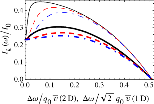
Figure 1: Relative intensity of the single lasing mode for the two-dimensional (2D) chaotic laser [Eq. (60), thick curves] and a one-dimensional (1D) laser [Eq. (82), thin curves] as a function of the frequency separation $\Delta\omega$ from the atomic-line center. The scaling of $\Delta\omega$ for these systems differs by a factor of $\sqrt{2}$ (see the text). Parameters: relative pumping strength $\Delta N_{0}/\Delta N_{0,k}=1.3$; relative homogeneous linewidth $\gamma_{\perp}/q_{0}\overline{v}=0.01$ (solid curves), $0.04$ (dashed curves), and $0.07$ (dash-dotted curves).

The results for the chaotic laser are compared in Fig. 1 with the relative mode intensity in a one-dimensional gas laser (B). In the former (latter) case, $\Delta\omega$ is normalized by $q_{0}\overline{v}$ ($\sqrt{2}q_{0}\overline{v}$). Apart from the visual convenience, the difference in scaling is motivated by the relation, $\overline{v}_{\text{2D}}=\sqrt{2}\,\overline{v}_{\text{1D}}$, between the root mean square velocities in two and one dimensions at a given temperature. Lasers with uniaxial resonators exhibit a much narrower intensity minimum, known as Lamb dip [1]. Its width is of the order of the homogeneous linewidth $\gamma_{\perp}\ll q_{0}\overline{v}$. In order to understand the origin of the dip, it is convenient to treat the lasing mode as a superposition of left- and right-moving waves. The atoms moving with the velocity $v_{x}\approx\Delta\omega/q_{x}$ effectively interact with only one of the two waves, depending on the sign of $\Delta\omega$ and $v_{x}$. However, when $|\Delta\omega|\lesssim\gamma_{\perp}$, the atoms at rest interact with both running waves. This leads to a stronger gain saturation near $\Delta\omega=0$ than away from the line center. In the two-dimensional chaotic laser this effect is washed out, since a mode with the frequency $\omega$ draws its gain from a larger ensemble of atoms with velocities $v>|\Delta\omega|/q_{0}$. In particular, let us model the chaotic wavefunction locally by a random superposition of partial plane waves with wavevectors of fixed magnitude $\sqrt{\epsilon}\,\omega/c$ and isotropically distributed directions [16]. Then, all partial waves of the central mode $\omega=\nu$ shall interact with the atoms at rest, but each partial wave interacts, in addition, with atoms moving perpendicular to its direction of propagation. Thus, the minimum of intensity results from a more subtle interplay of linear amplification and nonlinear saturation on the same frequency scale.

The results obtained above for a wave-chaotic resonator cannot be directly applied to resonators with mixed or regular classical ray dynamics, where the hypothesis of random, isotropically distributed, and uncorrelated eigenstates is no longer valid. Nevertheless, one can conjecture that increasing dimensionality of the system will make the intensity minimum shallower and wider (its depth and width being defined relatively to the intensity maximum and the inhomogeneous linewidth, respectively), but will not lead to its complete disappearance. As a practical consequence, the frequency stabilization [4] and spectroscopy [5] might still be possible in imperfect quasi-one-dimensional resonators, where the lasing mode deviates from a superposition of two counter-propagating plane waves. It is worth mentioning that in both uniaxial and chaotic resonators the relative depth of the minimum decreases with increasing $\gamma_{\perp}$.

5 Conclusions

In the present article, the semiclassical laser theory was extended to gas lasers with two-dimensional resonators of arbitrary shape. It was shown that the linear coupling between the modes, resulting from the Doppler shift in the gain frequency dependence, is negligible. The nonlinear coupling was considered in the third order of the perturbation theory in the electric field. The nonlinear terms in the laser equations that arise due to pulsations of the population inversion were identified and neglected. The criterion $(\nu/c)\,\overline{v}\gg\gamma_{\parallel}$, allowing one to approximate the population inversion as constant, is usually well fulfilled ($\nu$ is the atomic-transition frequency and $\overline{v}$ is the average velocity).

The general theory was applied to lasers with two-dimensional weakly open resonators of wave-chaotic geometry. In the short-wavelength limit, the eigenfunctions of the resonator can be locally approximated by a superposition of plane waves with a fixed wavelength propagating in random directions. The applicability condition for this description can be estimated as $c/\nu\ll w\ll L$, where $L$ is the size of the resonator and $w$ is the width of the output window. The isotropic statistical characteristics of the eigenfunctions lead to decoupling of the field distribution from the Doppler-broadened gain curve in the nonlinear terms of the laser equations. The single-mode intensity, as a function of the laser frequency, has a local minimum at the frequency of the atomic transition. The width of the minimum scales approximately with the inhomogeneous broadening $(\nu/c)\,\overline{v}$ and only weakly depends on the homogeneous linewidth $\gamma_{\perp}$. This property distinguishes the intensity minimum in chaotic resonators from the Lamb dip in uniaxial resonators, which has the width of $\gamma_{\perp}\ll(\nu/c)\,\overline{v}$.

Appendix A Constant-flux quasimodes

We consider an open cavity with a real dielectric constant $\epsilon(\mathbf{r})=\text{ const}$ inside and $\epsilon=1$ outside of the system’s boundary. The constant-flux (CF) modes [12] $\psi_{k\omega}(\mathbf{r})$, depending on the parameter $\omega>0$, are defined as solutions of a non-Hermitian eigenvalue problem. Explicitly, the functions must satisfy the differential equation

$$-c^{2}\,\nabla^{2}\psi_{k\omega}=\omega^{2}\psi_{k\omega}$$ (66)

in the exterior of the cavity with the outgoing-wave boundary conditions at infinity, while inside the system the same mode satisfies a different equation:

$$-c^{2}\,\nabla^{2}\psi_{k\omega}=\epsilon\,\Omega_{k}^{2}(\omega)\psi_{k\omega}.$$ (67)

For any given value of $\omega$, the complex eigenfrequency $\Omega_{k}(\omega)$ is quantized [$k$ is a discrete (multi-)index labeling the modes], because the solutions are required to match smoothly at the interface.

The conjugate wavefunctions $\phi_{k\omega}(\mathbf{r})$ obey Eq. (66) with the incoming-wave boundary conditions outside the cavity and the equation

$$-c^{2}\,\nabla^{2}\phi_{k\omega}=\epsilon[\Omega_{k}^{2}(\omega)]^{*}\phi_{k\omega}.$$ (68)

inside the system. The CF quasimodes and their conjugates are biorthogonal, and can be chosen to satisfy the condition

$$\int_{\mathcal{I}}d\mathbf{r}\,\phi_{k\omega}^{*}(\mathbf{r})\,\psi_{k^{\prime}\omega}(\mathbf{r})=\delta_{kk^{\prime}},$$ (69)

where the integration is over the interior $\mathcal{I}$. A similar relation,

$$\frac{1}{(2\pi)^{2}}\int d\mathbf{q}\,\phi_{k\mathbf{q}\omega}^{*}\psi_{k^{\prime}\mathbf{q}\omega}=\delta_{kk^{\prime}},$$ (70)

is valid in the $\mathbf{q}$ representation, defined as in Eq. (9). Additionally, the wavefunctions possess the properties: $\phi_{k\omega}(\mathbf{r})=[\psi_{k\omega}(\mathbf{r})]^{*}$ and $\phi_{k\mathbf{q}\omega}=\psi_{k,-\mathbf{q},\omega}^{*}$.

A Fourier component $E_{\omega}(\mathbf{r})$ of the lasing field can be expanded in the CF modes as

$$E_{\omega}(\mathbf{r})=\epsilon^{-1/2}\sum_{k}a_{k\omega}\,\psi_{k\omega}(\mathbf{r}),$$ (71)

$$a_{k\omega}=\epsilon^{1/2}\int_{\mathcal{I}}d\mathbf{r}\,\phi_{k\omega}^{*}(\mathbf{r})\,E_{\omega}(\mathbf{r}).$$ (72)

When continued to the exterior, this expansion yields a wave at the frequency $\omega$ propagating in the free space away from the system. In the stationary lasing regime $\omega$ becomes restricted to a finite number of values corresponding to the frequencies of lasing modes. To guarantee the realness of the field $E(\mathbf{r},t)$, we need to extend the definition of the CF quasimodes to negative frequencies by

$$\psi_{k,-\omega}(\mathbf{r})=\phi_{k\omega}(\mathbf{r}),\quad\phi_{k,-\omega}(\mathbf{r})=\psi_{k\omega}(\mathbf{r}).$$ (73)

Since the eigenfunctions $\phi_{k\omega}(\mathbf{r})$ depend only on the squared complex frequency $\Omega_{k}^{2}(\omega)$, the frequencies $\Omega_{k}(\omega)$ are determined up to an overall sign. To describe the field distribution with the outgoing flux and no incoming flux, the sign is chosen according to the requirements:

$$\text{Re}[\Omega_{k}(\omega)]>0,\quad\text{Im}[\Omega_{k}(\omega)]<0\quad(\omega>0),$$ (74)

$$\Omega_{k}(-\omega)=-[\Omega_{k}(\omega)]^{*}.$$ (75)

In connection with the definition (73), this choice provides for negative $\text{Im}[\Omega_{k}(\omega)]$ for any $\omega$, as is expected from the decaying quasimodes.

Appendix B One-dimensional gas laser

We apply the general theory to a one-dimensional gas laser that was studied in detail in Ref. [1]. Specifically, we consider a resonator defined by $\epsilon=1$ in the region $0<x<L$, with a perfect mirror at $x=0$ and a weakly transmitting mirror at $x=L$. The quasimode eigenfunctions have the form

$$\psi_{k}(x)=\frac{e^{i\Omega_{k}x/c}}{i\sqrt{2L}}-\frac{e^{-i\Omega_{k}x/c}}{i\sqrt{2L}}\equiv\psi_{k}^{(+)}(x)+\psi_{k}^{(-)}(x),$$ (76)

where we approximate $q_{k}\equiv\text{Re}\,\Omega_{k}/c\approx\pi k/L$ ($k=1,2,\ldots$) and assume $\delta q_{k}\equiv-\text{Im}\,\Omega_{k}/c\ll q_{k}$. In principle, $\delta q_{k}$ can be determined by modeling the semitransparent mirror as a dielectric layer with large dielectric constant and solving Eqs. (66) and (67), but the specific value of $\delta q_{k}$ is not important for our purposes. In the $q$ representation, the functions

$$\psi_{kq}^{(\pm)}=\frac{1}{\sqrt{2L}}\,\frac{1-e^{-i(q\mp q_{k}\pm i\,\delta q_{k})L}}{q_{k}-i\,\delta q_{k}\mp q}$$ (77)

have a resonant dependence on $q$, peaked at $\pm q_{k}$ and having a width of $\delta q_{k}$.

As in the two-dimensional case, the velocity average of the homogeneous gain curve can be computed within the approximation (48). Averaging over the one-dimensional Maxwell distribution yields

$$\left<\mathcal{L}(\omega-qv)\right>_{v}=\sqrt{\frac{\pi}{2}}\,\frac{\gamma_{\perp}}{q\overline{v}}\exp\left[-\frac{1}{2}\left(\frac{\Delta\omega}{q\overline{v}}\right)^{2}\right].$$ (78)

The third-order contribution is obtained from Eq. (43), adapted to the one-dimensional case. The electric field can be represented as a superposition of the quasimode wavefunctions (77). The velocity averages depend on $q$ on a scale larger than $\delta q_{k}$, and can be pulled out of the integrals and evaluated at the resonant values of $q$. The integrals over the wavefunctions have a quite simple form in the coordinate representation:

$$\frac{1}{(2\pi)^{3}}\int\!dq\,dq^{\prime}\,dq^{\prime\prime}\,\psi_{k,-q}^{(\alpha)}\,\psi_{k^{\prime},q+q^{\prime}-q^{\prime\prime}}^{(\alpha^{\prime})}\,\left[\psi_{k^{\prime\prime},q^{\prime}}^{(\alpha^{\prime\prime})}\right]^{*}\psi_{k^{\prime\prime\prime},q^{\prime\prime}}^{(\alpha^{\prime\prime\prime})}$$

$$=\int_{0}^{L}\!dx\,\psi_{k}^{(\alpha)}(x)\,\psi_{k^{\prime}}^{(\alpha^{\prime})}(x)\,\left[\psi_{k^{\prime\prime}}^{(\alpha^{\prime\prime})}(x)\right]^{*}\psi_{k^{\prime\prime\prime}}^{(\alpha^{\prime\prime\prime})}(x),$$ (79)

where $\alpha,\alpha^{\prime},\alpha^{\prime\prime},\alpha^{\prime\prime\prime}=+,-$ and we took into account that $\phi_{k}^{*}(x)=\psi_{k}(x)$. The phase of the integrand vanishes when the indices obey the resonance condition

$$\alpha k+\alpha^{\prime}k^{\prime}-\alpha^{\prime\prime}k^{\prime\prime}+\alpha^{\prime\prime\prime}k^{\prime\prime\prime}=0.$$ (80)

In the single-mode near-threshold regime, when only one quasimode is excited, six of the 16 possible combinations of indices are resonant. However, only four combinations, $(\alpha,\alpha^{\prime},\alpha^{\prime\prime},\alpha^{\prime\prime\prime})=(+-++)$, $(-+--)$, $(+---)$, $(-+++)$, yield $q^{\prime}=q^{\prime\prime}$ at resonance, which results in $D_{\parallel}=1$. In the limit $\delta q_{k}L\ll 1$, the resonant value of the integral (79) is equal to $1/4L$. The velocity averages in Eq. (43) with the resonant values of $q=\pm q_{k}$ and $q^{\prime}=q^{\prime\prime}\pm q_{k}$ sum up to $4\left<D(\omega-q_{k}v)\left[\mathcal{L}(\omega-q_{k}v)+\mathcal{L}(\omega+q_{k}v)\right]\right>_{v}$. This quantity was calculated in Ref. [1]. The real part in the Doppler limit is given by

$$\left<\mathcal{L}(\omega-qv)\left[\mathcal{L}(\omega-qv)+\mathcal{L}(\omega+qv)\right]\right>_{v}$$

$$=\sqrt{\frac{\pi}{8}}\,\frac{\gamma_{\perp}}{q\overline{v}}\exp\left[-\frac{1}{2}\left(\frac{\Delta\omega}{q\overline{v}}\right)^{2}\right]\left[1+\mathcal{L}(\omega)\right].$$ (81)

The imaginary part of Eq. (41) yields an expression for the mode intensity $I_{k}=|a_{lk}|^{2}$:

$$\frac{I_{k}(\omega)}{I_{0}}=2\,\frac{1-\frac{\Delta N_{0,k}}{\Delta N_{0}}\,e^{\frac{1}{2}\left(\frac{\Delta\omega}{q_{0}\overline{v}}\right)^{2}}}{1+\mathcal{L}(\omega)},$$ (82)

where we approximated $q_{k}\approx q_{0}$. The parameters

$$I_{0}=\frac{\hbar^{2}\gamma_{\perp}\gamma_{\parallel}L}{2d^{2}\nu},$$ (83)

$$\Delta N_{0,k}=\frac{\delta q_{k}\,\hbar\overline{v}L}{\sqrt{2}\,\pi^{3/2}\,d^{2}\mathcal{N}}$$ (84)

are defined in Sec. 4.2.

References

References

• [1] M. Sargent III, M. O. Scully, and W. E. Lamb, Jr. Laser Physics. Addison-Wesley, Reading, 1974.
• [2] H. Haken. Laser Theory. Springer, Berlin, 1984.
• [3] W. E. Lamb, Jr. Phys. Rev., 134:1429, 1964.
• [4] C. Freed and A. Javan. Appl. Phys. Lett., 17:53, 1970.
• [5] A. Szöke and A. Javan. Phys. Rev., 145:137, 1966.
• [6] H. Cao, Y. G. Zhao, S. T. Ho, E. W. Seelig, Q. H. Wang, and R. P. H. Chang. Phys. Rev. Lett., 82:2278, 1999.
• [7] R. C. Polson, A. Chipouline, and Z. V. Vardeny. Advanced Materials, 13:760, 2001.
• [8] T. S. Misirpashaev and C. W. J. Beenakker. Phys. Rev. A, 57:2041, 1998.
• [9] M. Patra, H. Schomerus, and C. W. J. Beenakker. Phys. Rev. A, 61:023810, 2000.
• [10] C. Viviescas and G. Hackenbroich. Phys. Rev. A, 67:013805, 2003.
• [11] L. I. Deych. Phys. Rev. Lett., 95:043902, 2005.
• [12] H. E. Türeci, A. D. Stone, and B. Collier. Phys. Rev. A, 74:043822, 2006.
• [13] O. Zaitsev and L. Deych. Phys. Rev. A, 81:023822, 2010.
• [14] O. Zaitsev and L. Deych. J. Opt., 12:024001, 2010.
• [15] M. V. Berry. J. Phys. A, 10:2083, 1977.
• [16] M. V. Berry. In G. Iooss, R. Helleman, and R. Stora, editors, Chaotic Behaviour of Deterministic Systems, page 171. North-Holland, Amsterdam, 1983.
• [17] O. Zaitsev. Phys. Rev. A, 76:043842, 2007.
• [18] L. Ge, R. J. Tandy, A. D. Stone, and H. E. Tureci. Opt. Exp., 16:16895, 2008.
• [19] H. E. Türeci, L. Ge, S. Rotter, and A. D. Stone. Science, 320:643, 2008. See also Supporting Online Material.
• [20] M. Abramowitz and I. A. Stegun, editors. Handbook of Mathematical Functions. Dover, New York, 1972.
• [21] L. E. Reichl. The Transition to Chaos: Conservative Classical Systems and Quantum Manifestations. Springer, New York, 2004.
• [22] L. Kaplan and E. J. Heller. Ann. Phys. (N.Y.), 264:171, 1998.