The event generator for the two-photon process
$e^{+}e^{-}\to e^{+}e^{-}R$ $(J^{PC}=0^{-+})$ in the single-tag mode

Abstract

The Monte Carlo event generator GGRESRC is described. The generator is developed for simulation of events of the two-photon process $e^{+}e^{-}\to e^{+}e^{-}R$, where R is a pseudoscalar resonance, $\pi^{0}$, $\eta$, $\eta^{\prime}$, $\eta_{c}$, or $\eta_{b}$. The program is optimized for generation of two-photon events in the single-tag mode. For single-tag events, radiative correction simulation is implemented in the generator including photon emission from the initial and final states.

1 Introduction

The purpose of this work is to develop an efficient event generator for the process of the two-photon resonance production $e^{+}e^{-}\to e^{+}e^{-}R$ in the so-called single-tag mode, when one of the final electrons is scattered at a large angle and detected. Such generator is needed for simulation of experiments on the measurement of the meson-photon transition form factors. The generator GGRESRC described in this work was used for the measurement of the transition form factors for the $\pi^{0}$, $\eta$, $\eta^{\prime}$, and $\eta_{c}$ mesons with the BABAR detector. To achieve required accuracy ($\sim 1\%$), the radiative corrections to the Born cross section are taken into account. In particular, extra photon emission from the initial and final states are simulated.

In the two-photon process $e^{+}e^{-}\to e^{+}e^{-}R$, the virtual photons, radiated by the colliding electrons, form a $C$-even resonance with the four-momentum ${k}={k}_{1}+{k}_{2}$ (see Fig. 1).

Figure 1: The diagram of the two-photon process $e^{+}e^{-}\to e^{+}e^{-}+R$.

Let $Q_{2}^{2}$ be the absolute value of the four-momentum squared, carried by the space-like photon connected with the tagged (detected) electron , while $Q_{1}^{2}$ be the same parameter for the untagged (undetected) electron ($Q_{1}^{2}\approx 0$). The transition form factor is determined from the measured differential cross section $({\rm d}\sigma/{\rm d}Q_{2}^{2})_{\rm data}$ and the MC calculated cross section $({\rm d}\sigma/{\rm d}Q_{2}^{2})_{\rm MC}$:

$$|{F}^{\rm data}_{\gamma^{*}\gamma R}(Q_{2}^{2})|^{2}=\frac{({\rm d}\sigma/{\rm d}Q_{2}^{2})_{\rm data}}{({\rm d}\sigma/{\rm d}Q_{2}^{2})_{\rm MC}}|{F}^{\rm MC}_{\gamma^{*}\gamma R}(Q_{2}^{2})|^{2},$$ (1)

where $|{F}^{MC}_{\gamma^{*}\gamma R}(Q_{2}^{2})|^{2}$ is the transition form factor used in MC simulation.

2 Born cross section

To describe the process $e^{+}e^{-}\to e^{+}e^{-}R$ we use the notations defined in Fig. 1, and the following six invariants:

$$t_{1}=-Q_{1}^{2}={k}_{1}^{2},\quad t_{2}=-Q_{2}^{2}={k}_{2}^{2},$$

$$s_{1}=({p}_{1}^{\prime}+{k})^{2},\quad s_{2}=({p}_{2}^{\prime}+{k})^{2},$$ (2)

$$s=({p}_{1}+{p}_{2})^{2},\quad W^{2}={k}^{2}=({k}_{1}+{k}_{2})^{2}.$$

The differential cross-section for this process in the lowest QED order is given by BGMS :

$${\rm d}\sigma=\frac{\alpha^{2}}{16\pi^{4}t_{1}t_{2}}\sqrt{\frac{({k}_{1}{k}_{2})^{2}-t_{1}t_{2}}{({p}_{1}{p}_{2})^{2}-m_{e}^{4}}}\Sigma\frac{{\rm d}^{3}\vec{p^{\prime}}_{1}}{E^{\prime}_{1}}\frac{{\rm d}^{3}\vec{p^{\prime}}_{2}}{E^{\prime}_{2}},$$ (3)

where $\alpha$ is the fine structure constant, $m_{e}$ is the electron mass, $E^{\prime}_{i}$ ($i$=1,2) are the energies of the scattered electrons and

$$\Sigma = 4\rho^{++}_{1}\rho^{++}_{2}\sigma_{TT}+2\rho^{++}_{1}\rho^{00}_{2}\sigma_{TS}+2\rho^{00}_{1}\rho^{++}_{2}\sigma_{ST}+\rho^{00}_{1}\rho^{00}_{2}\sigma_{SS}$$

$$+ 2|\rho^{+-}_{1}\rho^{+-}_{2}|\tau_{TT}\cos\,2\tilde{\phi}-8|\rho^{+0}_{1}\rho^{+0}_{2}|\tau_{TS}\cos\,\tilde{\phi}.$$

Here $\tilde{\phi}$ is the angle between the electron and positron scattering planes in the center-of-mass (c.m.) frame of the virtual photons, $\sigma_{ab}$ are the $\gamma^{\ast}\gamma^{\ast}\to R$ cross sections for unpolarized transverse ($a,b=T$) and scalar ($a,b=S$) photons. The interference terms containing the functions $\tau_{ab}$ arise due to virtual photon polarization. The function $\tau_{TT}$ is the difference between cross sections for transverse photons with the parallel and orthogonal linear polarizations: $\tau_{TT}=\sigma_{\parallel}-\sigma_{\perp}$, while the cross section for unpolarized photons is $\sigma_{TT}=(\sigma_{\parallel}+\sigma_{\perp})/2$.

The effects of the strong interaction are completely contained in the functions $\sigma_{ab}$ and $\tau_{ab}$. All other functions entering in Eq. (2) are calculable with QED. The expressions for the virtual photon density matrices $\rho^{++}_{i}$, $\rho^{+-}_{i}$, $\rho^{+0}_{i}$, $\rho^{00}_{i}$ ($i=1,2$) can be found in Ref. BGMS .

In the case of the pseudoscalar meson production, only the functions $\sigma_{TT}$ and $\tau_{TT}$ are non-zero, and $\tau_{TT}=-2\sigma_{TT}$ poppe . The cross section $\sigma_{TT}$ for a narrow pseudoscalar meson with the mass $M_{R}$ can be written in term of the transition form factor:

$$\sigma_{TT}(W,Q_{1}^{2},Q_{2}^{2})=8\pi\frac{\Gamma_{\gamma\gamma}}{M_{R}}\left|\frac{{F}(Q_{1}^{2},Q_{2}^{2})}{{F}(0,0)}\right|^{2},\,\,|{F}(0,0)|^{2}=\frac{4\Gamma_{\gamma\gamma}}{\pi\alpha^{2}M_{R}^{3}},$$ (5)

where $\Gamma_{\gamma\gamma}$ is the meson two-photon width. It should be noted that some two-photon event generators neglect the term with $\tau_{TT}$. This approach may be reasonable only for study of two-photon processes in the no-tag mode, when both the electrons are scattered at small angles. The $\tau_{TT}$ term gives a sizable contribution to the differential cross section ${\rm d}\sigma/{\rm d}Q_{2}^{2}$ at large $Q_{2}^{2}$ and should be taken into account in simulation of single-tag experiments.

In the GGRESRC events generator we perform integration of the differential cross section using invariant variables (2). For a narrow pseudoscalar resonance, Eq. (3) can be rewritten:

$${\rm d}\sigma=\frac{4\alpha^{2}\Gamma_{\gamma\gamma}}{\pi s^{2}t_{1}^{2}t_{2}^{2}M_{R}^{3}}\left|\frac{F(t_{1},t_{2})}{F(0,0)}\right|^{2}B\frac{{\rm d}t_{2}{\rm d}t_{1}{\rm d}s_{1}{\rm d}s_{2}}{\sqrt{-\Delta_{4}}},$$ (6)

where $\Delta_{4}(s,s_{1},s_{2},t_{1},t_{2},M_{R}^{2},m_{e}^{2})$ is the Gram determinant BK . The physical region in the variables $s_{1}$, $s_{2}$, $t_{1}$, $t_{2}$ is defined by the condition $\Delta_{4}\leq 0$. The function $B$ coincides, up to a factor, with the function $\Sigma$ (Eq. (2)) for pseudoscalar mesons. It was calculated in Ref. BKT and is given by

$$B=\frac{1}{4}t_{1}t_{2}B_{1}-4B_{2}^{2}+m_{e}^{2}B_{3},$$ (7)

where

$$B_{1} = (4{p_{1}}{p_{2}}-2{p_{1}}{k_{2}}-2{p_{2}}{k_{1}}+{k_{1}}{k_{2}})^{2}+({k_{1}}{k_{2}})^{2}-16t_{1}t_{2}-16m_{e}^{4},$$

$$B_{2} = ({p_{1}}{p_{2}})({k_{1}}{k_{2}})-({p_{1}}{k_{2}})({p_{2}}{k_{1}}),$$ (8)

$$B_{3} = t_{1}(2{p_{1}}{k_{2}}-{k_{1}}{k_{2}})^{2}+t_{2}(2{p_{2}}{k_{1}}-{k_{1}}{k_{2}})^{2}+4m_{e}^{2}({k_{1}}{k_{2}})^{2},$$

To describe the $Q_{1}^{2}$ and $Q_{2}^{2}$ dependencies of the transition form factor $F(Q_{1}^{2},Q_{2}^{2})$, the two options are implemented in the generator: $F(Q_{1}^{2},Q_{2}^{2})=F(0,0)$, and the vector-dominance model (VDM)

$$|F|^{2}=\frac{1}{(1+Q^{2}_{1}/\Lambda^{2})^{2}(1+Q^{2}_{2}/\Lambda^{2})^{2}},$$ (9)

where $\Lambda=m_{\rho}$ for $\pi^{0}$, $\eta$, $\eta^{\prime}$ production, $\Lambda=m_{J/\psi}$ for $\eta_{c}$, and $\Lambda=m_{\Upsilon}$ for $\eta_{b}$. The $Q_{2}^{2}$ dependence of the $|F|^{2}$ calculated with Eq. (9) at $Q_{1}^{2}=0$ for $\Lambda=m_{\rho}$, is shown in Fig. 2.

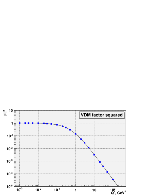
Figure 2: The $Q^{2}$ dependence of the form factor $|F|^{2}$ at $Q_{1}^{2}=0$, $\Lambda=m_{\rho}$=0.7755 GeV.

Four-dimensional Monte-Carlo integration of Eq. (6) is performed using the method developed for the GALUGA two-photon event generator S . In this method, in particular, the invariant variables are generated in the order $t_{2}$, $t_{1}$, $s_{1}$, $s_{2}$. This allows to set a restriction on $Q_{2}^{2}$ at the beginning of the event generation and significantly increase the generation efficiency for single-tag events. The values of the generated invariants, are then used together with a random azimuthal angle of the system of the final particles to calculate the 4-momenta of the scattered electron, positron, and produced resonance. The formulae to do this can be found in Ref. T . The main decay modes for $\pi^{0}$, $\eta$, and $\eta^{\prime}$ are also simulated according to Ref. T .

The total widths of the $\eta_{c}$ and $\eta_{b}$ resonances are comparable or even larger than the mass resolution of modern detectors. Therefore, the mass distributions for these resonances are generated using Breit-Wigner distributions.

3 Radiative correction

In the no-tag mode, when both the electron and the positron are scattered predominantly at small angles, the radiative correction to the Born cross section is expected to be small, less than 1% RC . The situation changes drastically in the single-tag mode, at a large electron scattering angle. At large $Q^{2}$ the correction due to extra photon emission from the initial state may reach several percents and should be taken into account in simulation.

The process-independent formula for the radiative correction in the next-to-leading order for two-photon processes in the single-tag mode was obtained in Ref. OK . The main contribution to the correction comes from the vertex of the tagged electron. The corresponding contribution of the untagged-electron vertex is expected to be smaller than 0.5% and neglected. Fig. 3 shows the diagrams taken into account in Ref. OK . They substitutes for the left-hand vertex in Fig. 1.

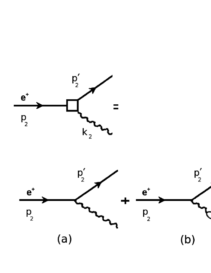
Figure 3: Diagrams used for calculation of the radiative correction.

The cross section for a single-tag experiment is given by:

$${\rm d}\sigma={\rm d}\sigma_{B}(1+\delta)={\rm d}\sigma_{B}(1+\delta^{\prime}+\delta_{VP}),$$ (10)

where ${\rm d}\sigma_{B}$ is the lowest-order cross section for the two-photon process given, for example, by Eq. (6). The total radiative correction is separated into two parts:

1. $\delta^{\prime}$, which includes the virtual correction due to the interference between the diagrams (a) and (c), soft-photon part of diagrams (d)+(e), and the corrections due to real photon emission from the initial (diagram (e)) and final (diagram (d)) states,

2. $\delta_{VP}$, the vacuum polarization correction due to the interference between the diagrams (a) and (b).

To obtain $\delta^{\prime}$ we have used the result of Ref. OK for the total radiative correction, removing from it the contribution of the vacuum polarization diagram, $\delta_{e}$ (in Ref. OK only electron contribution was taken into account). The resulting $\delta^{\prime}$ is given by

$$\delta^{\prime}=-\frac{\alpha}{\pi}\Biggl{\{}\biggl{[}\ln\frac{1}{r_{max}}-\frac{3}{4}\biggr{]}(L-1)+\frac{1}{4}\Biggr{\}}.$$ (11)

where $r_{max}$ ($\ll 1$) is the maximum energy of the photon emitted from the initial state in units of the beam energy $E_{b}$, $L=\ln{(Q^{2}/m_{e}^{2})}$, and $Q^{2}$ is the absolute value of the momentum transfer squared to the electron. The formula does not contain any restriction on the energy of the photon emitted from the final state, i.e. the cross section given by Eq. (10) is calculated for the case when the tagged electron is allowed to radiate a photon of any possible energy. The values of the correction $\delta^{\prime}$ for nine representative sets of $Q^{2}$ and ${r_{max}}$ are listed in Table 1.

Table 1: The correction $\delta^{\prime}$ (%) for the various values of $r_{max}$ and $Q^{2}$.

$Q^{2}$ (GeV2)	$r_{max}$=0.03	$r_{max}$=0.05	$r_{max}$=0.1
1	-9.1	-7.4	-5.2
10	-10.6	-8.6	-6.0
100	-12.1	-9.8	-6.8

In the $Q^{2}$ region from 1 to 100 GeV² available for experiments at $B$-factories, the correction reach 5–7% even with the relatively loose restriction ($r_{max}=0.1$) on the scaled energy of the undetected photon emitted from the initial state.

The correction $\delta^{\prime}$ is partly compensated by the vacuum polarization correction $\delta_{VP}$, for which we use the results of Ref. CMD-2 , which includes the contributions from the $e$, $\mu$, $\tau$ leptons, and hadrons. The $Q^{2}$ dependence of $\delta_{VP}$ is shown in Fig. 4 in comparison with $\delta_{e}$.

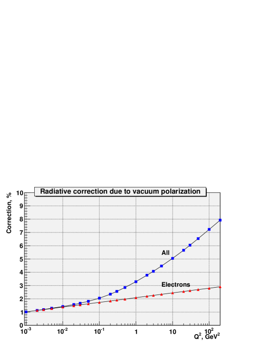
Figure 4: The vacuum polarization correction as a function of $Q^{2}$. The curve ”All” shows $\delta_{VP}$ calculated in Ref. CMD-2 with account of contributions from $e$, $\mu$, $\tau$, and hadrons. The curve ”Electrons” – represents the contribution only from electrons, $\delta_{e}$.

The values of the total correction $\delta=\delta^{\prime}+\delta_{VP}$ calculated for for nine representative sets of $Q^{2}$ and ${r_{max}}$ are listed in Table 2.

Table 2: Total radiative correction $\delta=\delta^{\prime}+\delta_{VP}$.

$Q^{2}$ (GeV 2)	$r_{max}$=0.03	$r_{max}$=0.05	$r_{max}$=0.1
1	-5.9	-4.3	-2.0
10	-5.6	-3.7	-1.0
100	-4.8	-2.6	+0.4

The emission of the hard photon by the electron distorts the kinematics of two-photon event. To model how this effect influences the detection efficiency, the event generator includes generation of extra photons emitted from the initial and final states.

3.1 Simulation of initial state radiation

For simulation of the initial state radiation (ISR), it is convenient to represent the radiative correction in the form

$$1+\delta^{\prime}\approx\left[1+\frac{\alpha}{\pi}\left(\frac{3}{4}L-1\right)\right]\int_{0}^{r_{max}}\frac{\beta dr}{r^{1-\beta}},$$ (12)

where $\beta=(\alpha/\pi)(L-1)$, $r=E_{\gamma}/E_{b}$, and $E_{\gamma}$ is the energy of the ISR photon.

The function under the integral can be interpreted as the energy spectrum for photons radiated from the initial state. Indeed, at $Q^{2}=1\div 100$ GeV² the parameter $\beta$ is small ($\beta=0.033\div 0.044$), and this function coincides approximately with the energy spectrum for hard photons, radiated from the initial state OK :

$$\frac{{\rm d}N}{{\rm d}r}=\frac{\alpha(L-1)}{\pi r}.$$ (13)

For simulation of the extra photon emission, we replace the four-dimensional integration in Eq. (6) to five-dimensional one with $r$ as the outermost integration variable

$${\rm d}\sigma=\left[1+\frac{\alpha}{\pi}\left(\frac{3}{4}L-1\right)\right]\frac{\beta}{r^{1-\beta}}{\rm d}\sigma_{B}{\rm d}r$$ (14)

The vacuum polarization correction is included by the substitution

$$\alpha^{2}\to\alpha^{2}(1+\delta_{VP}(Q_{1}^{2}))(1+\delta_{VP}(Q_{2}^{2}))$$ (15)

in the Born cross section ${\rm d}\sigma_{B}$.

In simulation of the initial state radiation, the approximation is used that the photon is emitted strictly along the initial direction of the radiating electron. Since the energy of the photon is restricted by the condition $r<r_{max}$, we expect that this approximation does not lead to a significant systematics in determination of the detection efficiency. Note that selection criteria used in data analysis should provide the fulfillment of the condition $r<r_{max}$ for both experimental and simulated events.

To increase simulation efficiency, the variable $r$ is initially generated according to the $\beta_{0}/r^{1-\beta_{0}}$ distribution with $\beta_{0}=\beta(Q^{2}_{min})$, where $Q^{2}_{min}$ is a lower bound on the tagged-electron $Q^{2}$ for simulated single-tag event. If the generated value of $r$ is higher than a threshold $r_{min}$, the photon is added to the list of final particles in an event. The scattered $e^{+}$ and $e^{-}$, and the pseudoscalar meson are then generated in the frame with the shifted c.m. energy of $2E_{b}\sqrt{1-r}$. If $r<r_{min}$, the photon is not generated, and the c.m. energy is not shifted, but the radiative correction factor in the cross section (see Eq. (14)) is calculated.

3.2 Simulation of final state radiation

The final state radiation (FSR) is simulated after the generation of the two-photon event. The final electron scattered at a large angle is “decayed” to $e+\gamma$ with some probability. The final-meson four-momentum is then modified to provide the energy and momentum balance. The probability of the emission of the photon with the energy greater than $E_{\gamma,min}$ equals

$$P(Q^{2},x_{min})=\frac{\alpha}{\pi(1+\delta^{\prime})}\biggl{[}(L-1)\ln\frac{1}{x_{min}}-\frac{3}{4}L+1\biggr{]},$$ (16)

where $x_{min}=E_{\gamma,min}/E$, and $E$ is the electron energy before FSR simulation. This formula is obtained by integration of the FSR photon spectrum given by Eq. (23) of Ref. OCK . The $Q^{2}$ dependence of the FSR probability calculated for $x_{min}=0.1$, 0.01 and 0.001 is shown in Fig. 5.

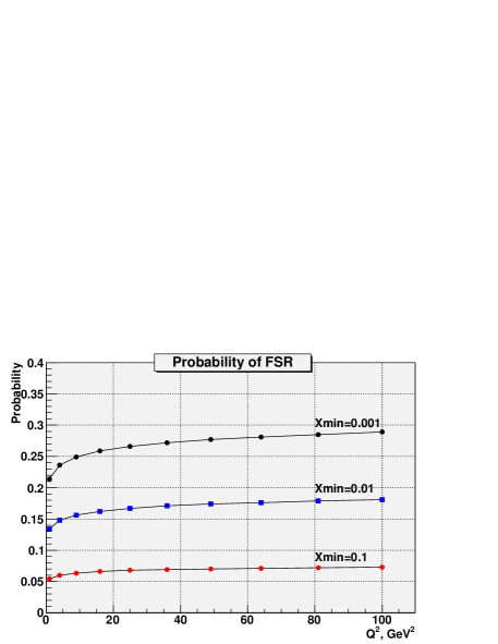
Figure 5: The $Q^{2}$ dependence of the final state radiation probability.

The photon energy $E_{\gamma}$ and angle $\theta_{\gamma}$ with respect to the electron direction before radiation are generated according to the following distribution function OCK :

$$\frac{{\rm d}N}{{\rm d}x{\rm d}\cos\theta_{\gamma}}=\frac{\alpha}{\pi x}\frac{1-x+x^{2}/2}{1-\beta\cos\theta_{\gamma}},\quad$$ (17)

where $x=E_{\gamma}/E$, $\beta=\sqrt{1-m_{e}^{2}/E^{\prime 2}}$, and $E^{\prime}$ is the electron energy after the photon emission.

4 Comparison with other generators

The comparison of the total cross sections in the no-tag mode obtained with GGRESRC and the two other generators of two-photon events, GGRESPS T and TWOGAM TWOGAM , was performed. The results of Monte-Carlo calculations are identical for all the three generators, if the mass of the meson, its two-photon width, and $Q^{2}$-dependence of the form factor are set to be the same in the generators. The GGRESRC and GGRESPS use the same formula (Eq. (6)), but different orders of integration over the invariant variables. The TWOGAM generator was developed for the CLEO measurements of the meson-photon transition form factors CLEO-2 . It is based on the BGMS formalism BGMS (see Eq. (3)) and uses the completely different integration variables, the momenta of the final electrons.

For GGRESRC in the regime without radiative corrections and TWOGAM, the comparison of the $Q^{2}$ spectra, obtained for the process of the $\pi^{0}$ production in the single-tag mode, was performed. The spectra was found to be in agreement within the Monte-Carlo statistical errors.

5 Generator parameters

The parameters of the event generator are listed in Table 3. The recommended values for the parameters Rmax, Rmin, and Kmin are given in brackets. To simulate no-tag events, the parameters Q1Smin, Q2Smin, and IRad should be set to zero. The regime with radiative correction (IRad=1) is used only in the single-tag mode.

Table 3: Parameters of the generator GGRESRC.

Name	Description
Eb	beam energy (GeV)
IR	produced meson: $\pi^{0}$ ($=1$), $\eta$ ($=2$), $\eta^{\prime}$ ($=3$), $\eta_{c}$ ($=4$), $\eta_{b}$ ($=5$)
IMode	meson decay mode (see Table 4)
KVMDM	form factor model: constant ($=0$), VDM ($=1$)
Itag	tagged particle: positron ($=1$), electron ($=2$), mix ($=3$)
IRad	simulation with/without radiative correction ($=1/0$)
Rmax	maximal energy of ISR photon in units of Eb ($0.1$)
Rmin	minimal energy of ISR photon in units of Eb ($10^{-4}$)
Kmin	minimal energy of the FSR photon ( 0.001 GeV )
Q1Smin	minimal momentum transfer squared to the untagged electron
Q1Smax	maximal momentum transfer squared to the untagged electron
Q2Smin	minimal momentum transfer squared to the tagged electron
Q2Smax	maximal momentum transfer squared to the tagged electron
Fmax	maximum weight of events

The resonances decay modes implemented in the generator are listed in Table 4. The decay models used are described in Ref. T . If parameter IMode equals 0, the meson decay is not simulated.

Table 4: The meson decay modes in GGRESRC. If IMode=0, the meson decay is not simulated.

Meson	IMode	Decay channel	Branching
			fraction PDG (%)
$\pi^{0}$	1	$\pi^{0}\to 2\gamma$	98.798
	2	$\pi^{0}\to e^{+}e^{-}\gamma$	1.198
	1	$\eta\to 2\gamma$	39.31
$\eta$	2	$\eta\to 3\pi^{0},\quad\pi^{0}\to 2\gamma$	31.4
	3	$\eta\to\pi^{+}\pi^{-}\pi^{0},\quad\pi^{0}\to 2\gamma$	22.457
	4	$\eta\to\pi^{+}\pi^{-}\gamma$	4.6
	1	$\eta^{\prime}\to 2\gamma$	2.1
$\eta^{\prime}$	2	$\eta^{\prime}\to\pi^{+}\pi^{-}\eta,\quad\eta\to 2\gamma$	17.532
	3	$\eta^{\prime}\to\pi^{+}\pi^{-}\eta,\quad\eta\to 3\pi^{0},\quad\pi^{0}\to 2\gamma$	14.004
	4	$\eta^{\prime}\to\pi^{+}\pi^{-}\eta,\quad\eta\to\pi^{+}\pi^{-}\pi^{0},\quad\pi^{0}\to 2\gamma$	10.016
	5	$\eta^{\prime}\to\pi^{+}\pi^{-}\eta,\quad\eta\to\pi^{+}\pi^{-}\gamma$	2.0516
	6	$\eta^{\prime}\to 2\pi^{0}\eta,\quad\eta\to 2\gamma,\quad\pi^{0}\to 2\gamma$	7.943
	7	$\eta^{\prime}\to 2\pi^{0}\eta,\quad\eta\to 3\pi^{0},\quad\pi^{0}\to 2\gamma$	6.3445
	8	$\eta^{\prime}\to 2\pi^{0}\eta,\quad\eta\to\pi^{+}\pi^{-}\pi^{0},\quad\pi^{0}\to 2\gamma$	4.5375
	9	$\eta^{\prime}\to 2\pi^{0}\eta,\quad\eta\to\pi^{+}\pi^{-}\gamma,\quad\pi^{0}\to 2\gamma$	0.9294
	10	$\eta^{\prime}\to\rho^{0}\gamma,\quad\rho^{0}\to\pi^{+}\pi^{-}$	29.4
$\eta_{c}$	1	$\eta_{c}\to K_{S}K^{+}\pi^{-}$ + c.c.	2.33
	2	$\eta_{c}\to 2\gamma$	0.024
$\eta_{b}$	1	$\eta_{b}\to 2\gamma$	-

In general terms the GGRESRC simulation algorithm is the following:

• The electron and positron collide in the c.m. frame ($S_{0}$). In this frame the positive $z$-axis is defined to coincide with the $e^{-}$ beam direction.

• The emission of a hard photon from the initial state is simulated. The photon is emitted along the collision axis. If the ISR photon energy is greater than $r_{min}E_{b}$, the photon momentum is stored in the list of final particles.

• The scattered electrons and the resonance are generated in the new c.m. frame ($S_{1}$) with the c.m. energy $2E_{b}\sqrt{1-E_{\gamma}/E_{b}}$; $S_{1}=S_{0}$ if $E_{\gamma}/E_{b}<r_{min}$.

• The final state radiation is simulated. If the photon energy is greater than $k_{min}$, its parameters are stored in the list of final particles. The momenta of the tagged electron and the produced meson are modified.

• The meson decay is simulated.

• The momenta of the final particles are transformed from $S_{1}$ to $S_{0}$ frame.

When required statistics is collected, the total cross section for the two-photon process with radiative corrections is calculated and printed.

Table 5: The simulation parameters used for calculation of the distributions shown in Figs. 6– 13.

Parameter	Value	Comment
Eb	5.29	beam energy (GeV)
IR	1	meson: $\pi^{0}$
IMode	1	decay mode: $\pi^{0}\to 2\gamma$
KVMDM	1	VDM form factor (Eq. (9)) is used
Itag	1	the final positron is tagged
IRad	1	radiative corrections are simulated
Rmax	0.1	maximal energy of ISR photons in units of $E_{b}$
Rmin	10-4	minimal energy of ISR photons in units of $E_{b}$
Kmin	0.001	minimal energy of FSR photons (GeV)
Q1Smin	0	$Q^{2}_{min}$ for $e^{-}$ (GeV2)
Q1Smax	1.5	$Q^{2}_{max}$ for $e^{-}$ (GeV2)
Q2Smin	1.5	$Q^{2}_{min}$ for $e^{+}$ (GeV2)
Q2Smax	9	$Q^{2}_{max}$ for $e^{+}$ (GeV2)

6 Example of $e^{+}e^{-}\to e^{+}e^{-}\pi^{0}$ simulation

In this section, some distributions for the process $e^{+}e^{-}\to e^{+}e^{-}+\pi^{0}$, $(\pi^{0}\to 2\gamma)$ obtained with the generator GGRESRC, are presented. In Table 5 the parameters of the generator used in the simulation are listed.

At these parameter values, 57% of events do not contain extra photons, 22%, 28%, and 6% of events contain ISR photon, FSR photon, and both ISR and FSR photons, respectively. The obtained cross section of the process and average radiative correction are: $\sigma=$0.99 pb, $\delta=$-0.6%.

The calculated cross section as a function of the restriction on $Q_{1}^{2}$ (the values of the other parameter are equal to those in Table 5) is shown in Fig. 6. One can see that at $Q_{1max}^{2}\approx$ 1.5 GeV² the cross section reaches an asymptotic value.

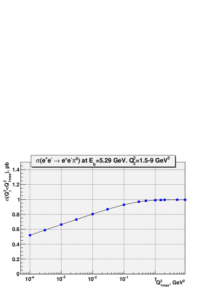
Figure 6: The $e^{+}e^{-}\to e^{+}e^{-}\pi^{0}$ cross section as a function of the limit on $Q_{1}^{2}$.

The energy spectra of tagged electrons obtained with and without radiative-correction simulation are shown in Fig. 7. It is seen that emission of extra photons significantly changes the shape of this spectrum.

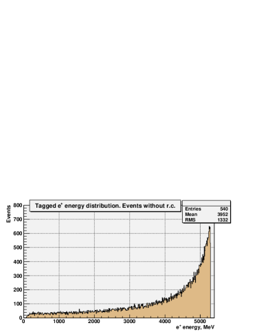
Figure 7: The energy spectra of tagged electrons from the process $e^{+}e^{-}\to e^{+}e^{-}\pi^{0}$ calculated without (left panel) and with (right panel) radiative correction simulation.

Fig. 8 shows the energy spectra of the photons from the $\pi^{0}\to 2\gamma$ decay in the process $e^{+}e^{-}\to e^{+}e^{-}\pi^{0}$. The energy spectra of photons emitted by the initial and final electrons are presented in Fig. 9.

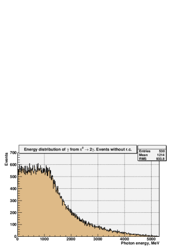
Figure 8: The energy spectra of photons from the $\pi^{0}\to 2\gamma$ decay in the process $e^{+}e^{-}\to e^{+}e^{-}\pi^{0}$ calculated without (left panel) and with (right panel) radiative correction simulation.

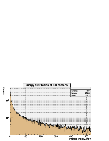
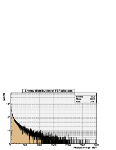
Figure 9: The energy spectrum of ISR (left panel) and FSR (right panel) photons in the simulation of the process $e^{+}e^{-}\to e^{+}e^{-}\pi^{0}$.

The polar-angle distributions of tagged electrons is shown in Figs. 10. It is seen that at $E_{b}=5.29$ GeV the cut $Q^{2}_{min}>1.5$ GeV² corresponds to the minimum scattering angle of about $13^{\circ}$. This is in agreement with an estimate for small scattering angles $\theta\approx Q/(E_{b}\cdot E^{\prime})^{1}/2$, where energy of the scattered electron $E^{\prime}\approx E_{b}$.

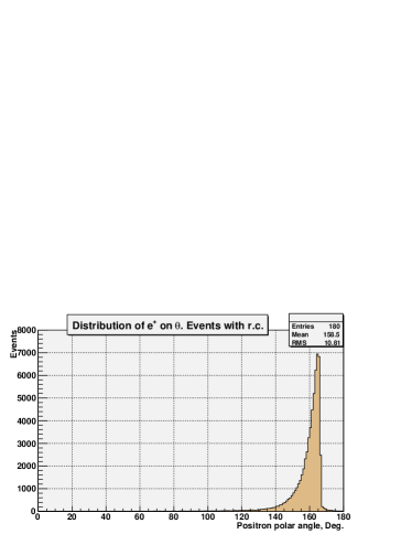
Figure 10: The polar-angle distributions of tagged electrons from the process $e^{+}e^{-}\to e^{+}e^{-}\pi^{0}$ obtained without (left panel) and with (right panel) radiative correction simulation.

The polar angle distribution of FSR photons is shown in Fig. 11. Since the FSR photon is emitted predominantly along the tagged-electron direction, the photon angular distribution is very close to that for the electron.

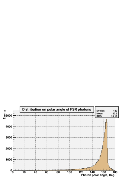
Figure 11: The polar-angle distributions of FSR photons from the process $e^{+}e^{-}\to e^{+}e^{-}\pi^{0}$.

The polar-angle distribution of photons from the $\pi^{0}\to 2\gamma$ decay is shown in Fig. 12. Photons have wide distribution, which becomes more uniform with account of radiative corrections.

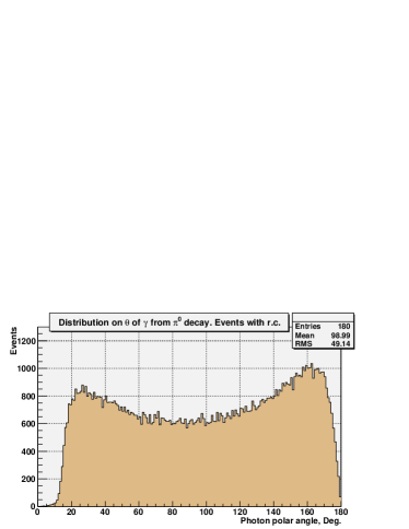
Figure 12: The polar-angle distributions of photons from the $\pi^{0}\to 2\gamma$ decay in the process $e^{+}e^{-}\to e^{+}e^{-}\pi^{0}$ obtained without (left panel) and with (right panel) radiative correction simulation.

In Fig. 13 the distribution of the missing mass in the process $e^{+}e^{-}\to e^{+}e^{-}+\pi^{0}$ is shown. The missing mass is calculated as $\sqrt{(p_{1}+p_{2}-k-p_{2}^{\prime})^{2}}$, i.e. we assume that only the tagged electron and the two photon from $\pi^{0}$ decay are detected. The narrow peak at zero mass contains events (57% of the total number of events), which do not have extra ISR or FSR photons. It is seen that emission of the extra photons leads to significant widening of the missing mass distribution.

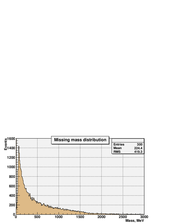
Figure 13: The missing mass distribution for the simulated $e^{+}e^{-}\to e^{+}e^{-}\pi^{0}$ single-tag events.

7 Program components

7.1 Common blocks

COMMON /GGRSTA/Sum,Es,Sum1,Sum2,Fm,Fm1,NOBR,Nact,Ngt

Purpose: to collect simulation statistics.
Sum Real*8 used for calculation of the total cross section
Es Real*8 used for calculation of the cross-section error
Sum1 Real*8 used for calculation of the average form factor
Sum2 Real*8 used for calculation of the average radiative correction factor
Fm Real*8 maximum weight of event
Fm1 Real*8 maximum weight of event in FSR simulation
NOBR Integer*4 number of calls of the generator
Nact Integer*4 number of the generated events
Ngt Integer*4 number of events with the weight greater than Fmax (see /GGRPAR/)

COMMON /GGRPAR/Eb,Rmas,Rwid,Rg,Rm,Fmax,Rmax,Rmin,t1imin,t1imax,
               t2imin,t2imax,Kmin,Fmax1,IR,IMode,KVMDM,ITag,IRad

Purpose: simulation parameters.
Eb Real*8 beam energy (GeV)
Rmas Real*8 meson mass (GeV)
Rwid Real*8 meson total width (GeV)
Rg Real*8 meson two-photon width (keV)
Rm Real*8 meson mass in the current event (GeV)
Fmax Real*8 expected maximum weight of event
Rmax Real*8 maximal energy of ISR photon in Eb units
Rmin Real*8 minimal energy of ISR photon in Eb units
t1imin Real*8 minimal value of $t_{1}$ (GeV²)
t1imax Real*8 maximal value of $t_{1}$ (GeV²)
t2imin Real*8 minimal value of $t_{2}$ (GeV²)
t2imax Real*8 maximal value of $t_{2}$ (GeV²)
Kmin Real*8 minimal energy of the FSR photon (GeV)
Fmax1 Real*8 maximum expected weight for FSR simulation
IR Integer*4 meson type
Imode Integer*4 meson decay mode
KVMDM Integer*4 form factor model
ITag Integer*4 tagged particle
IRad Integer*4 switch for radiative correction calculation

COMMON /GGRCON/Alpha,PI,EM,mPi0,mPi,mEta,mEtap,mKs,mKc,mRho,mJpsi,
               mUps,BrPi0(2),BrEta(4),BrEtaPrim(4),BrRho,BrTot

Purpose: constants.
Alpha Real*8 fine structure constant (1/137.03604)
Pi Real*8 $\pi$ (3.14159265)
Em Real*8 electron mass (0.00051099891 GeV)
mPi0 Real*8 $\pi^{0}$ mass (0.1349766 GeV)
mPi Real*8 $\pi^{\pm}$ mass (0.13957018 GeV)
mEta Real*8 $\eta$ mass (0.547853 GeV)
mEtap Real*8 $\eta^{\prime}$ mass (0.95766 GeV)
mKs Real*8 $K_{S}$ mass (0.497614 GeV)
mKc Real*8 $K^{\pm}$ mass (0.493677 GeV)
mRho Real*8 $\rho^{0}$ mass (0.77549 GeV)
mJpsi Real*8 $J/\psi$ mass (3.096916 GeV)
mUps Real*8 $\Upsilon$ mass (9.4603 GeV)
BrPi0(2) Real*8 $\pi^{0}$ decay branching fractions
BrEta(4) Real*8 $\eta$ decay branching fractions
BrEtaPrim(4) Real*8 $\eta^{\prime}$ decay branching fractions
BrRho Real*8 branching fraction of the decay $\rho^{0}\to\pi^{+}\pi^{-}$
BrTot Real*8 total probability of the decay chain

COMMON /GGREV/pPart(4,25),mPart(25),Type(25),Mother(25),Npart

Purpose: final particle parameters (up to 25 particles).
pPart(1-3,i) Real*8 momentum of i-th particle (GeV)
pPart(4,i) Real*8 energy of i-th particle (GeV)
mPart(i) Integer*4 mass of i-th particle (GeV)
Type(i) Integer*4 type of i-th particle
Mother(i) Integer*4 index of parent of i-th particle in /GGREV/
Npart Integer*4 total number of particles in /GGREV/

In the common block /GGREV/: 1-st and 2-nd particles are the scattered electrons, 3-rd particle is the produced resonance, 4-th e.t.c. particles are the ISR photon (if exists), the FSR photon (if exists), resonance decay products.

COMMON /GGRPOL/SETS(7330),SETPOL(7330)

Purpose: vacuum polarization correction.
SETS Real*8 momentum transfer squared (GeV²)
SETPOL Real*8 value of the vacuum polarization correction
Common blocks for internal use: /GGRARIP/, /GGRFUC/.

7.2 Subroutines of the generator

GGRESRC the main subroutine
GGRDEC2G simulation of resonance decay to 2$\gamma$
GGRESEND print out of simulation results
GGRESINI initialization
GGRETCD simulation of $\eta_{c}$ decays
GGRETD simulation of $\eta$ decays
GGRET1D simulation of $\eta^{\prime}$ decays
GGRET1D1 simulation of the decays $\eta^{\prime}\to\pi^{+}\pi^{-}\eta$ and $\pi^{0}\pi^{0}\eta$
GGRET1D2 simulation of the decay $\eta^{\prime}\to\rho^{0}\gamma$
GGRFSR FSR simulation
GGRFVP filling the common block /GGRPOL/
GGRINV simulation of the invariants $t_{2}$, $t_{1}$, $s_{1}$, $s_{2}$
GGRLMOM calculation of the laboratory momenta of the final electrons and meson
GGRLOR Lorentz transformation
GGRPI0D simulation of $\pi^{0}$ decays
GGRPI0D1 simulation of the $\pi^{0}\to e^{+}e^{-}\gamma$ decay
GGRPREV print out of one event
GGRRNDM wrapper of a pseudo-random numbers generator
GGRSPC3 simulation of the three particle phase space

7.3 Double-precision functions

GGRPOLAR calculation of the vacuum polarization correction
GGRFU function used by the subroutine GGRFSR
GGRFVMDM calculation of the form factor in the vector dominance model

7.4 Library subroutines

In the generator we use following functions from the CERN program library:
RANLUX generation of pseudo-random numbers uniformly distributed in the interval (0,1);
DZEROX computing a zero of a real-valued function $f(x)$ in the given interval [a, b].

8 Summary

The event generator GGRESRC for simulation of the two-photon process $e^{+}e^{-}\to e^{+}e^{-}R$, where $R$ is a pseudoscalar meson, has been developed. The generator allows to efficiently generate two-photon events in the single-tag mode, when one of the final electrons is scattered at a large angle and may be detected. In this mode simulation of radiative corrections has been implemented in the generator including extra photon emission from the initial and final states.

The generator is used for simulation of experiments with the BABAR detector on measurements of the photon-meson transition form factors (see, for example, Refs. Bab_pi0 ; Bab_etac ), and for simulation of two-photon experiments with the KEDR detector at VEPP-4M collider.

The work is partially supported by the RF Presidential Grant for Sc. Sch. NSh-6943.2010.2.

References

- (1) V. M. Budnev, I. F. Ginzburg, G. V. Meledin and V. G. Serbo, Phys. Rep. 15, 181 (1975).
- (2) M. Poppe, Int. J. Mod. Phys. A 1, 545 (1986).
- (3) E. Byckling, K. Kajante, Particle Kinematics (John Wiley & Sons Ltd., New York, 1973).
- (4) S. J. Brodsky, T. Kinoshita, H. Terazawa, Phys. Rev. D 4 (1971) 1532.
- (5) G. A. Schuler, Comput. Phys. Commun. 108, 279 (1998).
- (6) V.A.Tayursky, Preprint INP 2001-61. Novosibirsk 2001 (in Russian).
- (7) M. Defrise, S. Ong, J. Silva and C. Carimalo, Phys. Rev. D 23, 663 (1981); W. L. van Neerven and J. A. M. Vermaseren, Nucl. Phys. B 238, 73 (1984).
- (8) S. Ong and P. Kessler, Phys. Rev. D 38, 2280 (1988).
- (9) S. Ong, C. Carimalo and P. Kessler, Phys. Lett. B 142, 429 (1984).
- (10) F. V. Ignatov, PHD thesis, Budker INP 2008 (in Russian).
- (11) TWOGAM, The Two-Photon Monte Carlo Simulation Program, written by D. M. Coffman (unpublished).
- (12) J. Gronberg et al. [CLEO Collaboration], Phys. Rev. D 57, 33 (1998).
- (13) Particle Data Group, Phys. Lett. B 667, 1 (2008).
- (14) B. Aubert et al. [BABAR Collaboration], Phys. Rev. D 80, 052002 (2009).
- (15) J. P. Lees et al. [BABAR Collaboration], Phys. Rev. D 81, 052010 (2010).