Non-vanishing boundary effects and quasi-first order phase transitions in high dimensional Ising models

Abstract

In order to gain a better understanding of the Ising model in higher dimensions we have made a comparative study of how the boundary, open versus cyclic, of a $d$-dimensional simple lattice, for $d=1,\ldots,5$, affects the behaviour of the specific heat $\mathcal{C}$ and its microcanonical relative, the entropy derivative $-\partial S/\partial U$.

In dimensions 4 and 5 the boundary has a strong effect on the critical region of the model and for cyclic boundaries in dimension 5 we find that the model displays a quasi first order phase transition with a bimodal energy distribution. The latent heat decreases with increasing systems size but for all system sizes used in earlier papers the effect is clearly visible once a wide enough range of values for $K$ is considered.

Relations to recent rigorous results for high dimensional percolation and previous debates on simulation of Ising models and gauge fields are discussed.

I Introduction

The Ising model on 2 and 3-dimensional lattices is probably the most studied model in the theory of phase transitions from the condensed matter point of view. However, since at least the early 90’s higher dimensional lattices have become increasingly more important due to their connection to gauge field theory and particle physics. In particular the Ising model on the 4- and 5-dimensional cubic lattices have been studied both theoretically and via simulation. In these dimensions it is known that in the thermodynamical limit Aizenman (1982); Sokal (1979) the model follows the mean field critical exponents, but the finite size behaviour of the model has been hotly debated Brezin and Zinn-Justin (1985); Lai and Mon (1990); Mon (1996); Binder et al. (1985); Stevenson (2005); Balog et al. (2006); Chen and Dohm (1998a, b, 2000); Cea et al. (1998); Luijten et al. (1999a); Blöte and Luijten (1997); Luijten et al. (1999b). Part of the importance of these debates comes from the fact that it directly impinges on the methods used to derive other quantities from the finite size data, whose values are not already known in the limit. These methods e.g. affect what has been done in field theoretical studies of the Higgs particle mass as well as other properties studied using lattice quantum chromodynamics.

In the work presented here we set out to make a systematic comparison of the finite size behaviour of the Ising model on lattices with open and cyclic boundary conditions. We include both the well studied 2- and 3-dimensional lattices and the earlier debated lattices in dimension 4 and 5. To our knowledge the previous studies in higher dimensions have focused exclusively on lattices with cyclic boundary conditions, but as recent rigorous results on percolation Aizenman (1997); Heydenreich and van der Hofstad (2007) has shown, for this, simpler, model there are non-vanishing boundary effects in higher dimension. We believe that there is a risk in focusing only the cyclic case.

As our sampled data reveals, there is a striking change in how the boundary conditions affect the finite size behaviour as we pass the critical dimension $D=4$. For $D=4$ the finite size effects are more visible in the microcanonical ensemble than in the canonical. This is due to the smoothing effect of fluctuations in the energy of the system. Here the data, as previously shown in Lundow and Markström (2009a), favours the conclusion that the specific heat at $K_{c}$ is bounded, which is consistent with the rigorous result $\alpha=0$ but in conflict with predictions of a weak divergence by renormalization theory Brézin et al. (1976). We also find that for a certain range of small sizes and open boundary conditions the specific heat has two maxima close to the critical point, one of which disappears as the system size increases. In the microcanonical ensemble this effect remains visible even for the largest systems we have studied (L=40). For cyclic boundary conditions not such effects are visible in either ensemble.

For $D=5$, where the specific heat is rigorously known to be bounded Sokal (1979), the model display more striking differences between the two boundary conditions. As for the 4-dimensional case there is a system size range with two maxima in the specific heat for free boundary conditions, but not for the cyclic case. This effect is again visible for even larger size in the microcanonical ensemble, because the smoothing effect of energy fluctuations is not present here. There is also a larger gap between the effective critical points for each size, e.g. the values of $K$ at which the model has the maximum specific heat, but this is to be expected due to the relatively large boundary size. However, the most striking difference is that for cyclic boundary conditions the model displays a quasi-first order phase transition. For $K$ close to $K_{c}$ the energy distribution becomes bimodal, just as for a high-$q$ Potts model. As the system size increases the gap between the two maximima scales as $L^{-5/2}$, thereby giving the model an effective latent heat for finite size, but not in the thermodynamic limit. Due to this bimodal behaviour simulations become sensitive to small changes in $K$, as this makes the model favour one of the two maxima and thereby a different internal energy. In fact, some of the disagreements between different simulations and data mentioned in Brezin and Zinn-Justin (1985); Lai and Mon (1990); Mon (1996); Binder et al. (1985); Stevenson (2005); Balog et al. (2006); Chen and Dohm (1998a, b, 2000); Cea et al. (1998); Luijten et al. (1999a); Blöte and Luijten (1997); Luijten et al. (1999b) might be due to this overlooked effect.

II Notation

We will investigate the behaviour of two types of lattice graphs, the cartesian graph product of $d$ cycles, i.e. $C_{L}\times\cdots\times C_{L}$, and the product of $d$ paths $P_{L}\times\cdots\times P_{L}$ for $d=2,3,4,5$. Both types of graphs have $n=L^{d}$ vertices, the product of cycles has $d\,L^{d}$ edges and the product of paths has $d\,L^{d-1}\,(L-1)$ edges. They differ only at their boundaries where the cycle product has cyclic boundary conditions while the path product has open boundary conditions.

We define the energy of a state $\sigma=(\sigma_{1},\ldots,\sigma_{n})$, with $\sigma_{i}=\pm 1$, as $E(\sigma)=\sum_{\{i,j\}}\sigma_{i}\,\sigma_{j}$ (summation over the edges $\{i,j\}$), and the magnetisation as $M(\sigma)=\sum_{i}\sigma_{i}$ (summation over the vertices).

We look into two classes of quantities. The first of these, the combinatorial quantities from the microcanonical ensemble, provide an extremely detailed picture of the inner workings of the model, and they all depend on the energy $U=E/n$. The coupling $K$, defined as $K(U)=-\partial S/\partial U$, is of special interest here. Here $S(U)=(1/n)\,\ln a(E)$ where $a(E)$ denotes the number of states $\sigma$ at energy $E$. It is described in great detail in Häggkvist et al. (2004a) how to obtain these from sampled data.

The second class of quantities, the canonical (or physical) ones, are the cumulants, i.e. derivatives of $\ln\mathcal{Z}$ where $\mathcal{Z}$ is the partition function. How to obtain these quantities from the coupling function $K(U)$ is described in Lundow and Markström (2009b). We will refer to them in their dimensionless forms. We define the internal energy as $\mathcal{U}(K)=\left<E\right>/n$, the specific heat as $\mathcal{C}(K)=\mathrm{var}\left(E\right)/n$ and the susceptibility as $\chi(K)=\mathrm{var}\left(M\right)/n=\left<M^{2}\right>/n$. For each coupling $K$ we receive a distribution of energies having density function $\Pr{E}$ and again we refer the reader to Lundow and Markström (2009b) for how to obtain this distribution from the $K(U)$-function.

Occasionally we will, when necessary, subscript functions with the linear order $L$ of the lattice, as e.g. $\mathcal{C}_{L}(K)$. We denote by $K^{*}$ the coupling where $\mathcal{C}_{L}$ is at its maximum. We denote by $U^{*}$ an energy where $\partial K/\partial U$ has a local minimum and we use $U^{+}$ for a second minimum where $U^{*}<U^{+}$.

III 2D-lattices

For 2-dimensional lattices there is no qualitative difference between the cycle and the path product for the specific heat’s behaviour. In Figure 1 we plot the specific heat for both lattice types for a range of linear orders. Though the specific heat is somewhat smaller for the path products, not so strange considering that these graphs have fewer edges, the only substantial feature of the path products is that the peak is always located to the right of $K_{c}$ rather than to the left as it is for cycle products. We should here mention that for cycle products with $L\leq 320$ we rely on exact data computed in Häggkvist et al. (2004b) and for $L=512$ on sampled data. For path products we have exact data only for $L\leq 16$, see Lundow (1999), and sampled data otherwise.

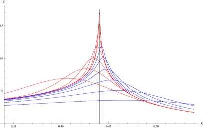
Figure 1: (Colour online) Specific heat $\mathcal{C}(K)$ for 2D cycle products (red) of linear order $L=8$, $16$, $32$, $64$, $128$, $256$, $512$ and for path products (blue) of linear order $L=8$, $16$, $32$, $64$, $128$, $256$. Black vertical line at $K_{c}=0.44068\ldots$.

Let us compare how the maximum specific heat grows. We know that for square cycle products the maximum grows as $1.03684+(8/\pi)\,\ln L$, and we extract this from Ferdinand and Fisher (1969). Note that for $C_{\infty}\times C_{L}$ the additive constant is instead $0.967550$, see Onsager (1944) for an exact expression. In Figure 2 we show $\max\mathcal{C}_{L}-(8/\pi)\,\ln L$ versus $1/L$ for both types of lattices. Though we do not know what the limit additive constant will be for path products we can estimate it to be $-2.30$.

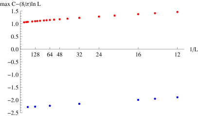
Figure 2: (Colour online) $\max\mathcal{C}_{L}-(8/\pi)\,\ln L$ vs $1/L$ for 2D cycle products (red points) of linear order $L=12$, $14$, $16$, $20$, $24$, $32$, $40$, $48$, $56$, $64$, $72$, $80$, $96$, $112$, $128$, $160$, $256$, $320$, $512$ and for path products (blue points) of linear order $L=12$, $14$, $16$, $32$, $64$, $128$, $256$.

The locations of the maxima are plotted in Figure 3. Note that the asymptotic behaviour is already known to be $K_{c}-K^{*}\sim 0.15878/L$, see Ferdinand and Fisher (1969), for the cycle products. For path products there are obviously some higher order correction terms at work as well.

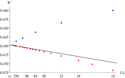
Figure 3: (Colour online) Location $K^{*}$ of maximum specific heat vs $1/L$ for 2D cycle products (red points) of linear order $L=16$, $20$, $24$, $32$, $40$, $48$, $56$, $64$, $72$, $80$, $96$, $112$, $128$, $160$, $256$, $320$, $512$ and for path products (blue points) of linear order $L=16$, $32$, $64$, $128$, $256$. The black asymptote is $K_{c}-0.15878/L$.

Looking from a microcanonical perspective and plotting the derivative $\partial K/\partial U$, which is effectively a microcanonical inverse of the specific heat, we see a more or less similar behaviour between the lattice types in Figure 4. This time the lattice types agree on which side of the asymptotic location the local minimum should be.

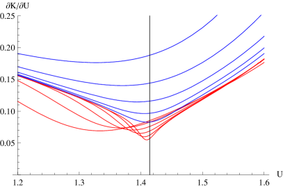
Figure 4: (Colour online) $\partial K/\partial U$ for 2D cycle products (red) of linear order $L=16$, $32$, $64$, $128$, $256$, $512$ and for path products (blue) of linear order $L=16$, $32$, $64$, $128$, $256$. Black line at $U_{c}=\sqrt{2}$.

For these lattices we can actually give the asymptotical behaviour for how the minimum of $\partial K/\partial U$ should approach $0$. Since the maximum specific heat grows as $(8/\pi)\,\ln L$, and we excpect no asymyptotic difference here between the lattice types, the minimum $\partial K/\partial U$ must vanish at exactly the inverse rate $\pi/(8\,\ln L)$. This is shown in Figure 5. Note that the path product lattices approach the asymptote from above and the cycle products from below.

Figure 5: (Colour online) $\min\partial K/\partial U$ for 2D cycle products (red points) of linear order $L=12$, $14$, $16$, $20$, $24$, $32$, $40$, $48$, $56$, $64$, $72$, $80$, $96$, $112$, $128$, $160$, $256$, $320$, $512$ and for path products (blue points) of linear order $L=12$, $14$, $16$, $32$, $64$, $128$, $256$. Black line is the asymptote $\pi/(8\,\ln L)$.

IV 3D-lattices

For 3-dimensional lattices we see no major difference in behaviour between the two lattices types either. In three dimensions we do not an exact solution to rely on, so we can not discern as many details as for 2D-lattices. For cycle products we have sampled data for $L=6,8,12,16,32,64,128,256,512$, as used in Häggkvist et al. (2007) while for path products we have sampled data only for smaller lattices; $L=6,8,12,16,24,32,46,64,96,128$. For both lattice types we use exact data for $L=4$.

Again let us compare the lattice types. The specific heat is shown in Figure 6. As in the 2D-case the path products’ maximum specific heat is smaller. The location of the maximum approach $K_{c}$ from above for both lattice types, see Figure 7. However, for path products this maximum is located much farther away from $K_{c}$. The black curves in the plot were obtained from a best fit of all available data points to the simple scaling formula

$$K^{*}=c_{0}+c_{1}\,L^{-\lambda_{1}}+c_{2}\,L^{-\lambda_{2}}$$ (1)

where we pre-ordained $c_{0}=0.2216546$ as found in Häggkvist et al. (2007). For the cycle products we received $c_{1}=0.3775$, $\lambda_{1}=1.654$, $c_{2}=-0.6169$ and $\lambda_{2}=2.297$. For the path products this gave $c_{1}=2.292$, $\lambda_{1}=1.617$, $c_{2}=-2.101$ and $\lambda_{2}=1.961$. The fitted curves agree beautifully with the points for all $L$ and they are included in the plot.

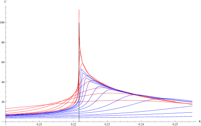
Figure 6: (Colour online) Specific heat $\mathcal{C}(K)$ for 3D cycle products (red) of linear order $L=4$, $6$, $8$, $12$, $16$, $32$, $64$, $128$, $256$, $512$ and for path products (blue) of linear order $L=4$, $6$, $8$, $12$, $16$, $24$, $32$, $48$, $64$, $96$, $128$. Black vertical line at $K_{c}\approx 0.2216546$.

3D $16$, $64$,

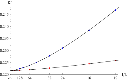
Figure 7: (Colour online) Location $K^{*}$ of maximum specific heat for 3D cycle products (red) of linear order $L=4$, $6$, $8$, $12$, $16$, $32$, $64$, $128$, $256$, $512$ and for path products (blue) of linear order $L=4$, $6$, $8$, $12$, $16$, $24$, $32$, $48$, $64$, $96$, $128$. See text for parameters of fitted curves.

On the microcanonical side we note that the derivative $\partial K/\partial U$ is much smaller for cycle products than for path products, see Figure 8. In Figure 9 we show the minimum values for both lattice types. Note that for cycle products this minimum is actually increasing for $L<16$, whereas for path products they are consistently decreasing. This decrement speeds up dramatically, as it should, for $L>64$ as shown in the figure.

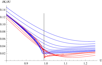
Figure 8: (Colour online) $\partial K/\partial U$ for 3D cycle products (red) of linear order $L=6$, $8$, $12$, $16$, $32$, $64$, $128$, $256$, $512$ and for path products (blue) of linear order $L=6$, $8$, $12$, $16$, $24$, $32$, $48$, $64$, $96$, $128$. Black line at $U_{c}\approx 0.99063$.

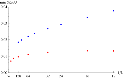
Figure 9: (Colour online) Minimum $\partial K/\partial U$ for 3D cycle products (red) of linear order $L=6$, $8$, $12$, $16$, $32$, $64$, $128$, $256$, $512$ and for path products (blue) of linear order $L=6$, $8$, $12$, $16$, $24$, $32$, $48$, $64$, $96$, $128$.

V 4D-lattices

In Lundow and Markström (2009a) the authors studied the Ising model on cycle products and, unexpectedly, found that the specific heat seemed to be bounded at $K_{c}$, a result which is compatible with the rigorous bounds but in disagreement with non-rigorous renormalization predictions. As we shall now see, unlike in the lower dimensional cases, in 4 dimensions there are also distinct differences in the finite size behaviour of the cycle and path products. In short, the specific heat of the path and cycle products differ somewhat in their behaviour, however on the microcanonical side larger differences are clearly visible. The minimum of $\partial K/\partial U$ at $U^{*}$ is much higher for path products and is decreasing with $L$, compared to the cycle products where it is actually increasing. Also, for $L\geq 12$ there is a second local minimum in $\partial K/\partial U$ at $U^{+}$, where $U^{*}<U^{+}$. This minimum becomes a global minimum for $L\geq 24$. We will now proceed as for the other lattices.

The specific heat is shown in Figure 10. Note especially the peculiar behaviour of $\mathcal{C}$ near $K^{*}$ for the path products. This is a phenomenon due to the extra local minimum at $U^{+}$ in $\partial K/\partial U$. Due to this peculiarity the location of the global maximum will display an irregular behaviour, depicted in Figure 11.

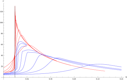
Figure 10: (Colour online) Specific heat $\mathcal{C}(K)$ for 4D cycle products (red) of linear order $L=4$, $6$, $8$, $12$, $16$, $24$, $32$, $40$, $48$, $64$, $80$ and for path products (blue) of linear order $L=4$, $6$, $8$, $12$, $16$, $24$, $32$, $40$. Black vertical line at $K_{c}\approx 0.1496947$.

In Figure 11 we have fitted curves to $K^{*}$ that are forced to have the same $c_{0}=K_{c}=0.1496947$, obtained in Lundow and Markström (2009a), and obviously there is no conflict in this. However, the correct asymptotic behaviour for the path products is only obtained from $L\geq 16$, for our choice of lattice sizes, leaving us only four points to fit our curve to. Thus we set $c_{2}=0$ in both cases and obtain $c_{1}=0.243$ and $\lambda_{1}=2.03$ for the cycle products. For the path products we obtain $c_{1}=0.166$ and $\lambda_{1}=0.962$. Strikingly, the exponents differ by about a factor two.

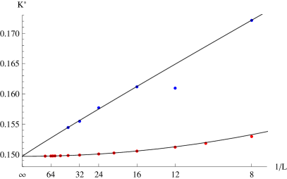
Figure 11: (Colour online) Location $K^{*}$ of the maximum specific heat $\mathcal{C}(K)$ for 4D cycle products (red) of linear order $L=4$, $6$, $8$, $10$, $12$, $16$, $20$, $24$, $32$, $40$, $48$, $56$, $60$, $64$, $80$ and for path products (blue) of linear order $L=4$, $6$, $8$, $12$, $16$, $24$, $32$, $40$.

Let us now turn to the microcanonical side. In Figure 12 we show $\partial K/\partial U$ for both lattice types, near $U_{c}$, where each curve has a local minimum. Outside the picture there also materialises, for path products with $L\geq 12$, a second local minimum, see Figure 13. This minimum is not as sharp as the other minimum, thus making it difficult to pin-point it to a high accuracy. Moreover, this minimum becomes a global minimum for $L\geq 24$. This phenomenon is shown in Figure 14.

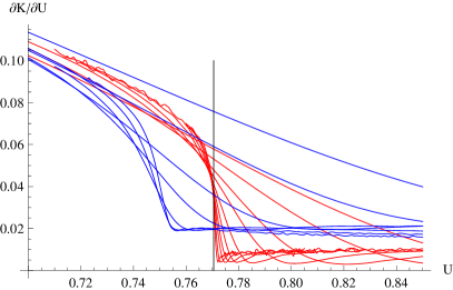
Figure 12: (Colour online) $\partial K/\partial U$ for 4D cycle products (red) of linear order $L=4$, $6$, $8$, $12$, $16$, $24$, $32$, $40$, $48$, $64$, $80$ and for path products (blue) of linear order $L=4$, $6$, $8$, $12$, $16$, $24$, $32$, $40$. Black line at $U_{c}\approx 0.770527$.

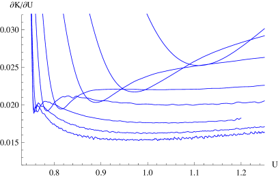
Figure 13: (Colour online) $\partial K/\partial U$ for 4D path products of linear order $L=4$, $6$, $8$, $12$, $16$, $24$, $32$, $40$.

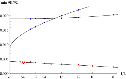
Figure 14: (Colour online) Minimum value of $\partial K/\partial U$ for 4D cycle products (red, converging to $0.004$) of linear order $L=4$, $6$, $8$, $10$, $12$, $16$, $20$, $24$, $32$, $40$, $48$, $56$, $60$, $64$, $80$ and for path products (blue) of linear order $L=4$, $6$, $8$, $12$, $16$, $24$, $32$, $40$. The blue points converging to $0.019$ are the minima located at $U^{*}$ and those converging to $0.009$ are located at $U^{+}$.

Here the picture gets more complicated. First, as was demonstrated in Lundow and Markström (2009a), the values of the local (and only) minima for the cycle products are increasing to about $0.0042$, thus leading to an asymptotically finite specific heat. As discussed in discussed in Lundow and Markström (2009a) this is in disagreement with a prediction from renormalization theory, which predicts a logarithmic singularity in the specific heat for $D=4$. It is rigorously known Sokal (1979) that the ciritcal exponent $\alpha=0$ for $D=4$. In Lundow and Markström (2009a) data from both a single spin Metropolis and a Wolff-cluster algorithm Wolff (1989) were compared to rule out methodological errors and the conclusion was that either systems as large as $L=80$ are still dominated by finite size effects or the renormalization prediction fails for the $D=4$ case, which is known to be the critical dimension for the nearest neighbour Ising model.

Second, the local minimum nearest $U_{c}$ for the path products seems to approach a different and even greater value of roughly $0.019$. Third, the other local minimum for the path products, also becoming a global minimum, could approach yet another value of about $0.009$ in between the other two. Forcing this minimum to approach the same minimum as for the cycle products seems out of the question with our current set of data though.

In Figure 14 the fitted curves a la (1) use $c_{2}=0$ and we received $c_{0}=0.0042$, $c_{1}=-0.016$, when setting $\lambda_{1}=1$ for the cycle products, see a discussion on this in Lundow and Markström (2009a). For the first set of local minima for the path products, the ones nearest $U_{c}$ we received $c_{0}=0.0190$, $c_{1}=0.223$, $\lambda_{1}=2.47$. The second set for the path products, farther away from $U_{c}$, gave us $c_{0}=0.00870$, $c_{1}=0.0568$, $\lambda_{1}=0.583$ when the curve was fitted to all data points.

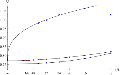
Figure 15: (Colour online) Location $U^{*}$ of the minimum value of $\partial K/\partial U$ for 4D cycle products (red points) of linear order $L=4$, $6$, $8$, $10$, $12$, $16$, $20$, $24$, $32$, $40$, $48$, $56$, $60$, $64$, $80$ and for path products (blue points) locations $U^{*}$ and $U^{+}$ for linear order $L=4$, $6$, $8$, $12$, $16$, $24$, $32$, $40$.

In Figure 15 we show the location of the local minima for both graph types. The location of the minima for the cycle products are clearly approaching $U_{c}\approx 0.770527$, see Lundow and Markström (2009a). However, the local minimum $U^{*}$ for the path products does not appear to approach the same limit for our current set of points. We believe this is only due to the lattices being too small; our current record size is only $L=40$ for the path products. The second minimum’s location $U^{+}$ could very well be the same as for the cycle products limit minimum location. An alternative possible scenario is that the local minimum $U^{*}$ will indeed have a different limit than $U_{c}$, but that this does not effect the behaviour of the canonical quantities since their behaviour is guided by the global minimum, the location of which appears to approach $U_{c}$.

The location $U^{*}$ of the minimum for the cycle products were set to have the limit $c_{0}=U_{c}=0.770527$. This gave $c_{1}=4.14$ and $\lambda_{1}=1.77$ when setting $c_{2}=0$ and fitting to the ten largest lattice sizes. This looks very convincing. For the path products’ local minimum $U^{*}$ we received $c_{0}=0.7528$, i.e. a different limit, and $c_{1}=23.1$, $\lambda_{1}=2.39$ when using $c_{2}=0$ and fitting to the last five data points. The local minimum $U^{+}$, which is a global minimum for $L\geq 24$, gave an acceptably good fit using $c_{0}=U_{c}$, $c_{1}=0.788$, $\lambda_{1}=0.355$.

VI 5D-lattices

For the 5-dimensional lattice the difference in behaviour between path products and cycle products becomes even more pronounced. Let us begin with the specific heat as usual. As Figure 16 shows, the behaviour is similar to that of the 4-dimensional lattice.

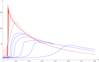
Figure 16: (Colour online) Specific heat $\mathcal{C}(K)$ for 5D cycle products (red) of linear order $L=4$, $6$, $8$, $10$, $12$, $16$, $20$, $24$ and for path products (blue) of linear order $L=4$, $6$, $8$, $12$, $16$, $20$. Black vertical line at $K_{c}\approx 0.113914$.

For these lattices the specific heat is rigorously known Sokal (1979) to be bounded. Using our scaling formula (1) with $c_{2}=0$ we received $c_{0}=172.8$, $c_{1}=-383.1$ and $\lambda_{1}=1.434$ giving an excellent fit over all the lattices. This is demonstrated by the red points and their fitted curve in Figure 17. Ideally we should also receive the same asymptotic value for the path products though the finite size scaling may be quite different. In the figure we have forced $c_{0}$ to the same value, $172.8$, as for the cycle products. This gave $c_{1}=-173.1$ and $\lambda_{1}=0.2222$. The fit does not look too strained, but forcing the value of $c_{0}$ was necessary for this.

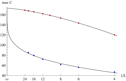
Figure 17: (Colour online) Maximum specific heat $\max\mathcal{C}(K)$ for 5D cycle products (red) of linear order $L=4$, $6$, $8$, $10$, $12$, $16$, $20$, $24$ and for path products (blue) of linear order $L=4$, $6$, $8$, $12$, $16$, $20$.

The locations of the maximum specific heat behave in the typical smooth fashion for the cycle products but the path products have the peculiar behaviour found in the 4D-lattice. Here, for $L\geq 8$ the maximum has jumped farther out from $K_{c}$. This shows clearly in Figure 18 where we plot the location of the maxima.

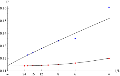
Figure 18: (Colour online) Location $K^{*}$ of the maximum specific heat $\mathcal{C}(K)$ for 5D cycle products (red) of linear order $L=4$, $6$, $8$, $10$, $12$, $16$, $20$, $24$ and for path products (blue) of linear order $L=4$, $6$, $8$, $12$, $16$, $20$.

For the fitted curves we have used $c_{0}=K_{c}=0.113914$, see Luijten et al. (1999b). Our best fit gave $c_{1}=0.183$ and $\lambda_{1}=2.44$ for the cycle products, but asymptotically we should have $\lambda_{1}=5/2$. For the path products we found $c_{1}=0.135$ and $\lambda_{1}=0.918$, based on the points for $L\geq 8$. The exponents thus differ considerably so there could be a different scaling rule in play here.

Moving on to the microcanonical side we show in Figure 19 the $\partial K/\partial U$-curves for the two types of lattices. As for the 4D-lattices we again see a huge qualitative difference between them. To begin with, for the path products we see a second local minimum in the curve, located far away from $U_{c}$, which becomes the global minimum for $L\geq 12$, see Figure 20. Also, the minima of the cycle products are all negative, whereas for the path products they are all positive. This is a striking difference, since a negative minimum is normally seen as an indication of a first-order phase transition, and as we shall see later there is indeed a first-order-like behaviour at the critical point for the cycle products.

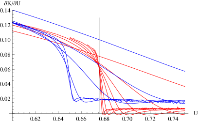
Figure 19: (Colour online) $\partial K/\partial U$ for 5D cycle products (red) of linear order $L=4$, $6$, $8$, $10$, $12$, $16$, $20$, $24$ and for path products (blue) of linear order $L=4$, $6$, $8$, $12$, $16$, $20$. Black line at $U_{c}\approx 0.67549$.

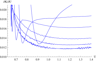
Figure 20: (Colour online) $\partial K/\partial U$ for 5D path products of linear order $L=4$, $6$, $8$, $12$, $16$, $20$.

As for the values of the minima we turn our eyes to Figure 21. The fitted curve for the cycle products has been forced to $c_{0}=0$, which may or may not be correct. Then $c_{1}$ took the best-fit value $-0.0054$ and $\lambda_{1}$ chose $0.447$, when setting also $c_{2}=0$. The point for $L=20$ was left out of the fitting process since it clearly deviates from the others in its behaviour.

For the path products we now have two sets of minima to look at, just as for the 4D-case. We run into trouble for the minima nearest $U_{c}$ though. Fitting (1) with only one exponent gave negative $\lambda_{1}$. This would imply that the minimum goes to infinity, which in its turn implies that the specific heat would go to zero. This is clearly an inconsistent behaviour due a too simple fit. Using two exponents instead, a best-fit gave $c_{0}=0.062$, $c_{1}=-0.071$, $c_{2}=0.042$, $\lambda_{1}=0.151$ and $\lambda_{2}=1.12$. The fit is very good. However, it should be kept in mind that this means we have fitted 5 parameters to 6 points, so the value of $c_{0}$ (as the other parameters) is likely to change upon receiving further data for larger lattices. What seems clear is that this minima has an increasing trend with increasing $L$.

Considering instead the minima farther out from $U_{c}$ we see in the figure that it becomes a global minimum for $L\geq 12$. Also, this local minimum only exists for $L\geq 8$. The fitted curve, setting $c_{2}=0$, has the parameters $c_{0}=0.0073$, $c_{1}=0.044$, $\lambda_{1}=0.77$, which gives a convincing fit but it relies on only 4 points.

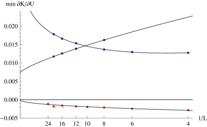
Figure 21: (Colour online) Minimum value of $\partial K/\partial U$ for 5D cycle products (red points) of linear order $L=4$, $6$, $8$, $10$, $12$, $16$, $20$, $24$ and for path products (two sets of blue points) of linear order $L=4$, $6$, $8$, $12$, $16$, $20$. The blue points converging to $0.06$ (outside the plot) are the minima at $U^{*}$ and the blue points converging to $0.007$ are the minima at $U^{+}$.

Figure 24 displays the location $U^{*}$ of the minimum $\partial K/\partial U$-values. For the path products we thus see two sets of these, $U^{*}$ and $U^{+}$. The curve fitted to the red points, i.e. the cycle products, has been forced to $c_{0}=U_{c}=0.67549$ and this gave $c_{1}=5.67$ and $\lambda_{1}=2.34$. Setting $c_{0}$ to $U_{c}$ for the path products’ minima at $U^{*}$ gave the curve a very strained look. A free fit instead gave $c_{0}=0.6478$, $c_{1}=13.6$ and $\lambda_{1}=2.67$. Receiving different limit values (which we also did for the 4D-lattice) is a rather unsatisfactory outcome, but the data points are very nicely fitted to this curve, and looks good even if we were to zoom in on these points only. More likely, the lattices are far too small to have received a correct asymptotic behaviour. However, we should not rule out the possibility of a second asymptotic critical point. After all, what matters to the model is that the global minimum goes to the same value as for the cycle products. This minimum’s location $U^{+}$ is also seen in the figure but it is very far from $U_{c}$. The curve through the last three points only, has a forced $c_{0}=U_{c}=0.67549$ and this gave $c_{1}=0.946$ and $\lambda_{1}=0.218$.

One focus of the earlier mentioned debates regarding the 5-dimensional Ising model Chen and Dohm (2000); Luijten et al. (1999a) was the scaling with $L$ of the susceptibility at $K_{c}$. Here the main term in the scaling has been predicted Binder et al. (1985); Privman and Fisher (1983) to be $L^{5/2}$ for cyclic boundary conditions, whereas an ordinary scaling would have been proportional to $L^{1/\nu}=L^{2}$. In addition Chen and Dohm (2000) predicted that there should be additional terms leading to a maximum in $\chi/L^{5/2}$ at $L=9$ after which it should decrease to a non-zero limit, a prediction which was criticized in Luijten et al. (1999a). Given our current, larger, data set we have made a brief return to this question, for both boundary conditions. In Figure 22 we see $\chi/L^{5/2}$ for several values of $K$ close to $K_{c}$. That the quotient is converging to a finite non-zero limit seems quite plausible for a range of possible $K_{c}$, but with the limited system sizes available to us it is hard to say what the limit should be. In Chen and Dohm (2000); Luijten et al. (1999a) data for $K=0.1139150$ were used, corresponding to the orange points in our figure. However, this value is larger than our best estimate and as the figure shows the quotient is extremely sensitive to even small changes in the value of $K_{c}$. The data does support a maximum in the quotient, but a location at $L=12$ seems more likely than the $L=9$ predicted in Chen and Dohm (2000).

In Figure 23 we plot the quotient $\chi/L^{2}$, corresponding to $\chi/L^{1/\nu}$ , for open boundary conditions. We see an excellent agreement over the full range of system sizes. We thus conclude that for open boundary conditions the dominant term in the scaling is $L^{2}$ and that any correction terms are significantly smaller. Experiments also showed that this quotient was much less sensitive to the value of $K_{c}$ than for cyclic boundaries.

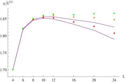
Figure 22: (Colour online)$\chi/L^{5/2}$ vs $L$ for 5D cycle products of linear order $L=4,6,8,10,12,16,20,24$ at $K=0.1139139$ (red points), $K=0.1139150$ (orange points), $K=0.1139155$ (green points). The purple lines correspond to the upper and lower ends of the estimate $K_{c}=0.1139139(5)$.

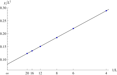
Figure 23: (Colour online)$\chi/L^{2}$ vs $1/L$ for 5D path products of linear order $L=4,6,8,12,16,20$ at $K=0.1139139$ (blue points). The line has slope $0.825$ and the asymptotic value is $0.0821$.

Figure 24: (Colour online) Location $U^{*}$ of the minimum value of $\partial K/\partial U$ for 5D cycle products (red points) of linear order $L=4$, $6$, $8$, $10$, $12$, $16$, $20$, $24$ and for path products ($U^{*}$ and $U^{+}$) of linear order $L=4$, $6$, $8$, $12$, $16$, $20$. The points at $U^{+}$ are above those at $U^{*}$.

VI.1 The nature of the phase transition for the cycle products

The 5-dimensional cycle products are quite exceptional since the $\partial K/\partial U$ become negative. This is then obviously reflected in the function $K(U)$ by having a local maximum and a local minimum. This, in turn, means that the distribution of energies becomes bimodal for a range of temperatures, see Touchette et al. (2004); Lundow and Markström (2009b) for discussions from the mathematical and computational perspectives respectively. A bimodal energy distribution is normally the clearest sign of first-order, or discontinuous, phase transition, with a latent heat given by the distance between the two maxima of the energy distrubution. For $D>4$ the Ising model has been rigorously proven Aizenman (1981, 1982) to have a second-order phase transition with critical exponents given by the mean field model. Hence we here see a clear difference between the asymptotic and finite size behaviour, which we will now examine closer.

In Figure 25 we show the normalised distributions at the temperature where the two distribution peaks are equal and the inset picture shows a zoomed-in plot clearly demonstrating that the distributions are indeed bimodal. Denoting the location of the local maxima of this bimodal distribution as $U_{1}$ and $U_{2}$ their difference goes to zero as roughly $U_{2}-U_{1}\sim 6.2/L^{5/2}$. The right maximum $U_{2}$ behaves as roughly $U_{c}+13/L^{5/2}$. The temperature where the maxima of the distribution are of equal height scales as $K_{c}+0.12/L^{5/2}$.

These results mean that for finite $L$ we see an effective latent heat with size proportional to $L^{-5/2}$ and, as for other models with a first order phase transition in their thermodynamic limit, the finite size model demonstrates a bistable behaviour at $K_{c}$. This behaviour is noticeable in the simulations, where the system will spend a long time at one maximum and then rapidly switch to the other.

Given the scaling of $U_{2}-U_{1}$ we find it quite possible that the model will display this bimodal distribution for all finite $L$ and only reach the pure mean field behaviour in the thermodynamic limit $L\rightarrow\infty$.

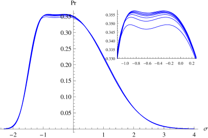
Figure 25: (Colour online) Normalised distribution of energies at the temperature where the two peaks of the density function are equal, for 5D cycle products of linear order $L=4$, $6$, $8$, $10$, $12$, $16$, $20$, $24$ (blue). The inset picture shows a zoomed-in version.

The density function of the energy distribution for the cycle products undergoes some dramatic shape-shifting near $K_{c}$. It starts as a gaussian function, then becomes heavily skewed to the left, then bimodal, then skewed to the right, and finally it becomes gaussian again. In Figure 26 we show this as a gallery of distributions for $L=16$ near $K_{c}$.

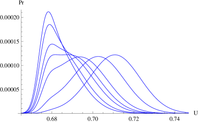
Figure 26: (Colour online) Density functions for the 5D cycle products $L=16$ near $K_{c}$ at $K=0.11396$, $0.11398$, $0.11401$, $0.114027$, $0.11405$, $0.11410$, $0.11415$ (left to right).

The path products on the other hand, for which $\partial K/\partial U$ stays positive, clearly can not have a bimodal distribution. Consequently, the density function has a rather non-spectacular behaviour near $K_{c}$ as Figure 27 shows. Even at the temperature where the specific heat is at its maximum the distribution stays quite gaussian. However, at the temperature range where specific heat grows most quickly, there is some typical behaviour. For example, the usual left-to-right skewness is found, but it is considerably less pronounced than for the cycle products.

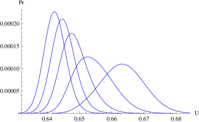
Figure 27: (Colour online) Density functions for the 5D path products $L=16$ near $K_{c}$ at $K=0.1164$, $0.1166$, $0.1168$, $0.1170$, $0.1172$ (left to right).

VII Conclusions

As we have seen, the finite size behaviour of the Ising model becomes significantly more complex as we pass the critical dimension $D=4$. In the case of 4 dimensions we have found that an additional maximum in the specific heat appears for a certain range of sizes, but only for open boundary conditions. We also found that both the cyclic and open cases seem to favour a bounded specific heat, with a value which they approach from below and above respectively, thereby contradicting a prediction from renormalization theory Brézin et al. (1976).

Some of the peculiarities of the 4-dimensional cases appears in the 5-dimensional model as well, but here the most striking feature is the quasi first order phase transition for cyclic boundary conditions. The presence of this, for the Ising model, unusual phase transition type, has numerous implications for Monte Carlo experiment and their analysis.

1. The model is highly sensitive to small changes in $K$. In Figure 26 the two curves closest to the bimodal one corresponds to the values $K=0.11401$ and $K=0.11405$. Here changes in the 5th decimal gives a significant change in the expected internal energy of the model.

2. Simulations at values $K$ at the balanced bimodal value will display a meta-stable behaviour, in which the models will stay for some time at one maximum and then rapidly change to the other.

3. Unlike what was initially hoped, the Wolff-cluster algorithm Wolff (1989) suffers from critical slowing down at first-order phase transitions, as was rigorously proven in C.Borgs et al. (1999). This means that, just as for the Metropolis algorithm, additional care must be taken in the study of this model in order to make sure that the generated data does not suffer from unwanted correlations

4. If only the moments of the energy distribution are studied at a given temperature the clearly non-gaussian form of the energy distribution can potentially lead to incorrect conclusions regarding higher moments based on the low order moments. There will e.g. be significantly non-zero odd moments for a longer interval of $K$ near $K_{c}$.

As we mentioned in the introduction the finite size behaviour of the simple percolation model has also been studied in higher dimensions. In Aizenman (1997) Aizenman found that the size of the largest cluster at $p_{c}$ scales, at most, as $L^{4}$ and conjectured that for cyclic boundary condition the scaling should be of order $L^{2d/3}$ instead. Recently this conjecture was proven in Heydenreich and van der Hofstad (2007), apart from a logarithmic factor which was removed in a follow up paper by the same authors hovedenreich and van der Hofstad (2009).

The general assumption in simulation physics is that as the system grows larger the effect of the boundary should diminish and the model converge to the same thermodynamic limit independently of the choice of boundary condition and the rough shape of the finite region. Following the seminal work of van Hove van Hove (1949) we know that for a large class of models this will be the case, but it is worth to notice that van Hove’s proof does in fact not apply to a sequence of larger and larger lattices with cyclic boundary conditions, as the proof assumes that the edge and vertices of the smaller lattices are subsets of those of the larger. However, for $K$ well away from $K_{c}$ we see no reason to expect anything else. Nonetheless, as the percolation results indicate, it is quite plausible that when we stay at, or near, $K_{c}$ we will see drastically different scalings depending on the choice of boundary conditions.

Generalizing the conjecture of Aizenman Aizenman (1997) we pose the following conjecture for the $q\geq 1$ random cluster model Fortuin and Kasteleyn (1972)

Conjecture 1

There exists a constant $c(q)$ and a dimenison $D(q)$ such that for the random cluster model with $q\geq 1$ and $d\geq D(q)$, the largest cluster in the $d$-dimensional cycle product with side $L$ contains $L^{c(q)d}$ vertices at $p_{c}(q)$.

The case $q=1$ corresponds to percolation and $q=2$ to the Ising model. We intend to return to this conjecture in an upcoming paper.

For models more complicated than the Ising model, such as those from QCD Cea et al. (1998); Stevenson (2005); Balog et al. (2006), quantitative differences between different boundary conditions have certainly been expected. The unexpected appearance of qualitative differences in the nature of the finite-size phase transition, such as what we have seen for $D=5$, poses a more serious problem. Close to a phase transition point different boundary conditions can potentially lead to quite distinct asymptotics, thereby making it necessary to study more than one kind of boundary in order to help pinpoint the correct infinite system asymptotics.

On a more general note we believe that the sensitivity to $K$ displayed in Figure 22 clearly demonstrates why single value simulations of models no longer suffice for studying models at the level of accuracy needed in modern physics. Instead methods allowing a continuous variation of the system parameters after the simulation, such that of Häggkvist et al. (2004a), are needed. The authors of Luijten et al. (1999a) stated that ”for a full understanding of the problem a variation of parameters over a broad range is desirable” and looking at our current findings we most emphatically agree.

References

- Aizenman (1982) M. Aizenman, Comm. Math. Phys. 86, 1 (1982), ISSN 0010-3616.
- Sokal (1979) A. D. Sokal, Phys. Lett. A 71, 451 (1979).
- Brezin and Zinn-Justin (1985) E. Brezin and J. Zinn-Justin, Nucl. Phys. B 257, 867 (1985).
- Lai and Mon (1990) P. Y. Lai and K. K. Mon, Phys. Rev. B 41, 9257 (1990).
- Mon (1996) K. K. Mon, Europhys. Lett. 34, 399 (1996).
- Binder et al. (1985) K. Binder, M. Nauenberg, V. Privman, and A. P. Young, Phys. Rev. B 31, 1498 (1985).
- Stevenson (2005) P. Stevenson, Nuclear Physics B 729, 542 (2005).
- Balog et al. (2006) J. Balog, F. Niedermayer, and P. Weisz, Nuclear Physics B 741, 390 (2006).
- Chen and Dohm (1998a) X. S. Chen and V. Dohm, International Journal of Modern Physics C 9, 1007 (1998a), eprint arXiv:cond-mat/9711298.
- Chen and Dohm (1998b) X. S. Chen and V. Dohm, International Journal of Modern Physics C 9, 1073 (1998b), eprint arXiv:cond-mat/9809394.
- Chen and Dohm (2000) X. S. Chen and V. Dohm (2000), eprint cond-mat/0005022.
- Cea et al. (1998) P. Cea, L. Cosmai, and M. Consoli, Modern Physics Letters A 13, 2361 (1998), eprint arXiv:hep-lat/9805005.
- Luijten et al. (1999a) E. Luijten, K. Binder, and H. Blöte, The European Physical Journal B - Condensed Matter and Complex Systems 9, 289 (1999a), ISSN 1434-6028, 10.1007/s100510050768, URL http://dx.doi.org/10.1007/s100510050768.
- Blöte and Luijten (1997) H. W. J. Blöte and E. Luijten, EPL (Europhysics Letters) 38, 565 (1997), URL http://stacks.iop.org/0295-5075/38/i=8/a=565.
- Luijten et al. (1999b) E. Luijten, K. Binder, and H. W. J. Blöte, Eur. Phys. J. B 9, 289 (1999b).
- Aizenman (1997) M. Aizenman, Nuclear Phys. B 485, 551 (1997), ISSN 0550-3213, URL http://dx.doi.org/10.1016/S0550-3213(96)00626-8.
- Heydenreich and van der Hofstad (2007) M. Heydenreich and R. van der Hofstad, Comm. Math. Phys. 270, 335 (2007), ISSN 0010-3616, URL http://dx.doi.org/10.1007/s00220-006-0152-8.
- Lundow and Markström (2009a) P. H. Lundow and K. Markström, Phys. Rev. E 80, 031104 (2009a).
- Brézin et al. (1976) E. Brézin, J. C. Le Guillou, and J. Zinn-Justin, in Phase transitions and critical phenomena, Vol. 6 (Academic Press, London, 1976), pp. 125–247.
- Häggkvist et al. (2004a) R. Häggkvist, A. Rosengren, D. Andrén, P. Kundrotas, P. H. Lundow, and K. Markström, J. Statist. Phys. 114, 455 (2004a).
- Lundow and Markström (2009b) P. H. Lundow and K. Markström, Cent. Eur. J. Phys. 7, 490 (2009b).
- Häggkvist et al. (2004b) R. Häggkvist, A. Rosengren, D. Andrén, P. Kundrotas, P. H. Lundow, and K. Markström, Phys. Rev. E 69, 046104 (2004b).
- Lundow (1999) P. H. Lundow, Tech. Rep. 14, Department of mathematics, Umeå university (1999), available at http://www.theophys.kth.se/~phl.
- Ferdinand and Fisher (1969) A. E. Ferdinand and M. E. Fisher, Phys. Rev. 185, 832 (1969).
- Onsager (1944) L. Onsager, Phys. Rev. (2) 65, 117 (1944).
- Häggkvist et al. (2007) R. Häggkvist, A. Rosengren, P. H. Lundow, K. Markström, D. Andrén, and P. Kundrotas, Adv. Phys. 56, 653 (2007).
- Wolff (1989) U. Wolff, Phys. Rev. Lett 62, 361 (1989).
- Privman and Fisher (1983) V. Privman and M. Fisher, Journal of Statistical Physics 33, 385 (1983), ISSN 0022-4715, 10.1007/BF01009803, URL http://dx.doi.org/10.1007/BF01009803.
- Touchette et al. (2004) H. Touchette, R. S. Ellis, and B. Turkington, Phys. A 340, 138 (2004), news and expectations in thermostatistics.
- Aizenman (1981) M. Aizenman, Phys. Rev. Lett. 47, 1 (1981), ISSN 0031-9007.
- C.Borgs et al. (1999) C.Borgs, J.Chayes, A. Frieze, J.H.Kim, P.Tetali, E.Vigoda, and V.Vu, Proceedings of FOCS ’99 pp. 218–229. (1999), preprint available at http://www.math.cmu.edu/~af1p/papers.html.
- hovedenreich and van der Hofstad (2009) M. hovedenreich and R. van der Hofstad, Probability Theory and Related Fields pp. 1–19 (2009), ISSN 0178-8051, 10.1007/s00440-009-0258-y, URL http://dx.doi.org/10.1007/s00440-009-0258-y.
- van Hove (1949) L. van Hove, Physica 15, 951 (1949).
- Fortuin and Kasteleyn (1972) C. M. Fortuin and P. W. Kasteleyn, Physica 57, 536 (1972).