Quantum Dot Spin Filter in Resonant Tunneling and Kondo Regimes

Abstract

A quantum dot with spin-orbit interaction can work as an efficient spin filter if it is connected to $N$ ($\geq 3$) external leads via tunnel barriers. When an unpolarized current is injected to a quantum dot from a lead, polarized currents are ejected to other leads. A two-level quantum dot is examined as a minimal model. First, we show that the spin polarization is markedly enhanced by resonant tunneling when the level spacing in the dot is smaller than the level broadening. Next, we examine the many-body resonance induced by the Kondo effect in the Coulomb blockade regime. A large spin current is generated in the presence of the SU(4) Kondo effect when the level spacing is less than the Kondo temperature.

The generation of spin current with no magnetic field or ferromagnets is an important issue for spin-based electronics, “spintronics.”[1] In this context, the spin-orbit (SO) interaction has attracted much interest. For conduction electrons in direct-gap semiconductors, an external potential $U({\bm{r}})$ results in the Rashba SO interaction[2, 3]

$$H_{\text{RSO}}=\frac{\lambda}{\hbar}{\bm{\sigma}}\cdot\left[{\bm{p}}\times{\bm{\nabla}}U({\bm{r}})\right],$$ (1)

where ${\bm{p}}$ is the momentum operator and ${\bm{\sigma}}$ is the Pauli matrices indicating the electron spin ${\bm{s}}={\bm{\sigma}}/2$. The coupling constant $\lambda$ is markedly enhanced by the band effect, particularly in narrow-gap semiconductors, such as InAs.[4, 5] The spatial inversion symmetry is broken in compound semiconductors, which gives rise to another type of SO interaction, the Dresselhaus SO interaction.[6] It is given by

$$H_{\text{DSO}}=\frac{\lambda^{\prime}}{\hbar}\bigl{[}p_{x}(p_{y}^{2}-p_{z}^{2})\sigma_{x}+p_{y}(p_{z}^{2}-p_{x}^{2})\sigma_{y}$$

$$+p_{z}(p_{x}^{2}-p_{y}^{2})\sigma_{z}\bigr{]}.$$ (2)

In the presence of SO interaction, the spin Hall effect (SHE) produces a spin current traverse to an electric field applied by the bias voltage. Two types of SHE have been intensively studied. One is an intrinsic SHE, which is induced by the drift motion of carriers in the SO-split band structures.[7, 8, 9] The other is an extrinsic SHE caused by the spin-dependent scattering of electrons by impurities.[10] Kato et al. observed the spin accumulation at sample edges traverse to the current,[11] which is ascribable to the extrinsic SHE with $U({\bm{r}})$ being the screened Coulomb potential by charged impurities in eq. (1).[12] In our previous studies,[13, 14] we theoretically examined the extrinsic SHE in semiconductor heterostructures due to the scattering by an artificial potential created by antidots, STM tips, and others. The potential is electrically tunable. We showed that the SHE is significantly enhanced by the resonant scattering when the attractive potential is properly tuned. We proposed a three-terminal spin-filter including a single antidot.

In the present letter, we study the enhancement of the “extrinsic SHE” by resonant tunneling through a quantum dot (QD) with a strong SO interaction, e.g., InAs QD.[15, 16, 17, 18] The QD is connected to $N$ external leads via tunnel barriers. In the QD, the number of electrons can be tuned, one by one, owing to the Coulomb blockade when the electrostatic potential is changed by the gate voltage $V_{\text{g}}$. The current through a QD shows a peak structure as a function of $V_{\text{g}}$ (Coulomb oscillation). We use the term SHE in the following meaning: For $N\geq 3$, when an unpolarized current is injected to the QD from a lead, polarized currents are ejected to the other leads. In other words, the QD works as a spin filter. First, we examine the SHE around the current peaks, where the resonant tunneling takes place. We show that the spin polarization is markedly enhanced when the energy-level spacing in the QD is smaller than the level broadening due to the tunnel coupling to external leads. Next, we examine the many-body resonance induced by the Kondo effect in the Coulomb blockade regime with spin 1/2 in the QD. We obtain a large spin current in the presence of the SU(4) Kondo effect when the level spacing is less than the Kondo temperature.

Figure 1: Model for a quantum dot connected to $N$ external leads ($N\geq 2$). The quantum dot has two energy levels, $\varepsilon_{j}$ ($j=1,2$), which are coupled to lead $\alpha$ by $V_{\alpha,j}$ [$\alpha=$S or D$n$, $n=1,\cdots,(N-1)$]. An unpolarized current is injected from lead S and ejected to the other leads. The spin-orbit interaction is present in the quantum dot.

We assume that the SO interaction is present only in the QD and that the level spacing in the QD is comparable to the level broadening $\Gamma$ ($\sim 1$ $\mathrm{meV}$), in accordance with experimental situations.[15, 16, 17, 18] The strength of SO interaction, $\Delta_{\text{SO}}$ in eq. (6), is approximately $0.2$ $\mathrm{meV}$.[16, 17, 18] As a minimal model, we examine two levels in the QD. Note that previous theoretical papers[19, 20, 21, 22] concerned the spin-current generation in a mesoscopic region, or an open QD with no tunnel barriers, in which many energy levels in the QD participate in the transport.

We examine a two-level Anderson model with $N$ $(\geq 2)$ leads, shown in Fig. 1. The energy levels in the QD are denoted by $\varepsilon_{1}$ and $\varepsilon_{2}$ before the SO interaction is turned on. In the absence of magnetic field, wavefunctions of the states, i.e., $\langle{\bm{r}}|1\rangle$ and $\langle{\bm{r}}|2\rangle$, can be real. In the case of Rashba SO interaction, the orbital part in eq. (1) is a pure imaginary operator, and hence it has off-diagonal elements only; $\langle 2|H_{\text{RSO}}|1\rangle=\text{i}{\bm{h}}_{\text{SO}}\cdot{\bm{\sigma}}/2$ with $\text{i}{\bm{h}}_{\text{SO}}/2=(\lambda/\hbar)\langle 2|({\bm{p}}\times{\bm{\nabla}}U)|1\rangle$. If the quantization axis of spin is taken in the direction of ${\bm{h}}_{\text{SO}}$, the Hamiltonian in the QD reads

$$H_{\text{dot}} = \sum_{\sigma=\pm 1}(d_{1,\sigma}^{\dagger},d_{2,\sigma}^{\dagger})\left(\varepsilon_{\text{d}}-\frac{\Delta}{2}\tau_{z}+\sigma\frac{\Delta_{\text{SO}}}{2}\tau_{y}\right)\left(\begin{array}[]{c}d_{1,\sigma}\\ d_{2,\sigma}\end{array}\right)$$ (6)

$$+H_{\text{int}},$$

where $d_{j,\sigma}^{\dagger}$ and $d_{j,\sigma}$ are the creation and annihilation operators of an electron with orbital $j$ and spin $\sigma$, respectively. $\varepsilon_{\text{d}}=(\varepsilon_{1}+\varepsilon_{2})/2$, $\Delta=\varepsilon_{2}-\varepsilon_{1}$, and $\Delta_{\text{SO}}=|{\bm{h}}_{\text{SO}}|$. The Pauli matrices, $\tau_{y}$ and $\tau_{z}$, are introduced for the pseudo-spin representing level $1$ or $2$. $H_{\text{int}}$ describes the Coulomb interaction between electrons. The same form of the QD Hamiltonian is derived similarly in the case of Dresselhaus SO interaction in eq. (2).[23] Note that the level spacing would be $\sqrt{\Delta^{2}+(\Delta_{\text{SO}})^{2}}$ in an isolated QD.

The state $|j\rangle$ in the QD is connected to lead $\alpha$ by tunnel coupling, $V_{\alpha,j}$ ($j=1,2$), which is real. The tunnel Hamiltonian is

$$H_{\text{T}} = \sum_{j=1,2}\sum_{\alpha,k,\sigma}(V_{\alpha,j}d_{j,\sigma}^{\dagger}c_{\alpha k,\sigma}+\text{h.c}.)$$ (7)

$$= \sum_{\alpha,k,\sigma}V_{\alpha}[(e_{\alpha,1}d_{1,\sigma}^{\dagger}+e_{\alpha,2}d_{2,\sigma}^{\dagger})c_{\alpha k,\sigma}+\text{h.c}.],$$

where $c_{\alpha k,\sigma}$ annihilates an electron with state $k$ and spin $\sigma$ in lead $\alpha$. $V_{\alpha}=\sqrt{(V_{\alpha,1})^{2}+(V_{\alpha,2})^{2}}$ and $e_{\alpha,j}=V_{\alpha,j}/V_{\alpha}$. We introduce a unit vector, ${\bm{e}}_{\alpha}=(e_{\alpha,1},e_{\alpha,2})^{T}$. $V_{\alpha}$ is controllable by electrically tuning the tunnel barrier, whereas ${\bm{e}}_{\alpha}$ is determined by the wavefunctions $\langle{\bm{r}}|1\rangle$ and $\langle{\bm{r}}|2\rangle$ in the QD and hardly controllable for a given current peak. ($\{{\bm{e}}_{\alpha}\}$ and $\Delta$ vary from peak to peak during the Coulomb oscillation. We can choose a peak with appropriate parameters for the SHE in experiments.)

We assume a single channel of conduction electrons in the leads. The total Hamiltonian is

$$H=\sum_{\alpha}\sum_{k,\sigma}\varepsilon_{k}c_{\alpha k,\sigma}^{\dagger}c_{\alpha k,\sigma}+H_{\text{dot}}+H_{\text{T}}.$$ (8)

The strength of the tunnel coupling is characterized by the level broadening, $\Gamma_{\alpha}=\pi\nu_{\alpha}(V_{\alpha})^{2}$, where $\nu_{\alpha}$ is the density of states in lead $\alpha$. We also introduce a matrix of $\hat{\Gamma}=\sum_{\alpha}\hat{\Gamma}_{\alpha}$ with

$$\hat{\Gamma}_{\alpha}=\Gamma_{\alpha}\left(\begin{array}[]{cc}(e_{\alpha,1})^{2}&e_{\alpha,1}e_{\alpha,2}\\ e_{\alpha,1}e_{\alpha,2}&(e_{\alpha,2})^{2}\end{array}\right).$$ (11)

An unpolarized current is injected into the QD from a source lead ($\alpha=$S) and output to other leads [D$n$; $n=1,\cdots,(N-1)$]. The electrochemical potential for electrons in lead S is lower than that in the other leads by $-eV_{\text{bias}}$. The current with spin $\sigma=\pm$ from lead $\alpha$ to the QD is written as

$$I_{\alpha,\sigma}=\frac{\text{i}e}{\pi\hbar}\int d\varepsilon\text{Tr}\{\hat{\Gamma}_{\alpha}[f_{\alpha}(\varepsilon)(\hat{G}^{\text{r}}_{\sigma}-\hat{G}^{\text{a}}_{\sigma})+\hat{G}^{<}_{\sigma}]\},$$ (12)

where $\hat{G}^{\text{r}}_{\sigma}$, $\hat{G}^{\text{a}}_{\sigma}$, and $\hat{G}^{<}_{\sigma}$ are the retarded, advanced, and lesser Green functions in the QD, respectively, in $2\times 2$ matrix form in the pseudo-spin space.[24] $f_{\alpha}(\varepsilon)$ is the Fermi distribution function in lead $\alpha$. In the absence of electron-electron interaction, $H_{\text{int}}$, the conductance into lead D$n$ with spin $\sigma$ is given by[25]

$$G_{n,\sigma}=\left.-\frac{\text{d}I_{\text{D}n,\sigma}}{\text{d}V_{\text{bias}}}\right|_{V_{\text{bias}}=0}=\frac{4e^{2}}{h}\text{Tr}[\hat{G}^{\text{a}}_{\sigma}(\varepsilon_{\text{F}})\hat{\Gamma}_{\text{D}n}\hat{G}^{\text{r}}_{\sigma}(\varepsilon_{\text{F}})\hat{\Gamma}_{\text{S}}],$$ (13)

where the QD Green function is

$$\hat{G}^{\text{r}}_{\pm}(\varepsilon)=\left[\left(\begin{array}[]{cc}\varepsilon-\varepsilon_{\text{d}}+\frac{\Delta}{2}&\pm\text{i}\frac{\Delta_{\text{SO}}}{2}\\ \mp\text{i}\frac{\Delta_{\text{SO}}}{2}&\varepsilon-\varepsilon_{\text{d}}-\frac{\Delta}{2}\end{array}\right)+\text{i}\hat{\Gamma}\right]^{-1}$$ (14)

and $\varepsilon_{\text{F}}$ is the Fermi energy.

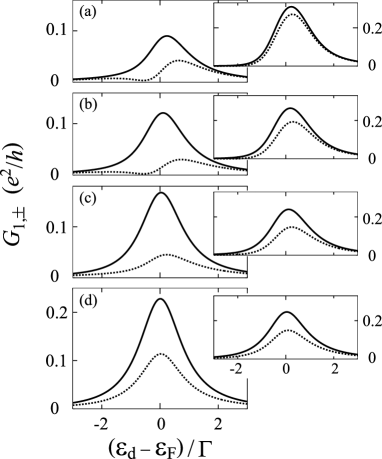
Figure 2: Calculated results of the conductance $G_{1,\pm}$ as a function of energy level, $\varepsilon_{\text{d}}=(\varepsilon_{1}+\varepsilon_{2})/2$, in a three-terminated quantum dot. Solid (broken) lines indicate the conductance $G_{1,+}$ ($G_{1,-}$) for spin $\sigma=+1$ ($-1$). The level broadening by the tunnel coupling to leads S and D$1$ is $\Gamma_{\text{S}}=\Gamma_{\text{D}1}\equiv\Gamma$ ($e_{\text{S},1}/e_{\text{S},2}=1/2$, $e_{\text{D}1,1}/e_{\text{D}1,2}=-3$), whereas that to lead D$2$ is (a) $\Gamma_{\text{D}2}=0.2\Gamma$, (b) $0.5\Gamma$, (c) $\Gamma$, and (d) $2\Gamma$ ($e_{\text{D}2,1}/e_{\text{D}2,2}=1$). $\Delta=\varepsilon_{2}-\varepsilon_{1}=0.2\Gamma$ in the main panels and $\Delta=\Gamma$ in the insets. $\Delta_{\text{SO}}=0.2\Gamma$.

Now, we discuss the SHE in the vicinity of the Coulomb peaks. The electron-electron interaction is neglected in this regime. From eqs. (13) and (14), we obtain

$$G_{n,\sigma} = \frac{e^{2}}{h}\frac{4\Gamma_{\text{S}}\Gamma_{\text{D}n}}{|D|^{2}}\left[g_{n}^{(1)}+g_{n,\sigma}^{(2)}\right],$$ (15)

$$g_{n}^{(1)} = \Biggl{[}\left(\varepsilon_{\text{F}}-\varepsilon_{\text{d}}-\frac{\Delta}{2}\right)e_{\text{D}n,1}e_{\text{S},1}$$ (16)

$$+\left(\varepsilon_{\text{F}}-\varepsilon_{\text{d}}+\frac{\Delta}{2}\right)e_{\text{D}n,2}e_{\text{S},2}\Biggr{]}^{2},$$

$$g_{n,\pm}^{(2)} = \Biggl{[}\pm\frac{\Delta_{\text{SO}}}{2}({\bm{e}}_{\text{S}}\times{\bm{e}}_{\text{D}n})_{z}$$ (17)

$$+\sum_{\alpha}\Gamma_{\alpha}({\bm{e}}_{\text{D}n}\times{\bm{e}}_{\alpha})_{z}({\bm{e}}_{\text{S}}\times{\bm{e}}_{\alpha})_{z}\Biggr{]}^{2},$$

where $D$ is the determinant of $[\hat{G}^{\text{r}}_{\sigma}(\varepsilon_{\text{F}})]^{-1}$ in eq. (14), which is independent of $\sigma$, and $({\bm{a}}\times{\bm{b}})_{z}=a_{1}b_{2}-a_{2}b_{1}$. Let us consider two simple cases. (I) When $\Delta\gg\Gamma_{\alpha}$ and $\Delta_{\text{SO}}$, $G_{n,\sigma}$ consists of two Lorentzian peaks as a function of $\varepsilon_{\text{d}}$, reflecting the resonant tunneling through one of the energy levels, $\varepsilon_{1,2}=\varepsilon_{\text{d}}\mp\Delta/2$:

$$G_{n,\sigma}\approx\frac{4e^{2}}{h}\Gamma_{\text{S}}\Gamma_{\text{D}n}\sum_{j=1,2}\frac{(e_{\text{D}n,j}e_{\text{S},j})^{2}}{(\varepsilon_{j}-\varepsilon_{\text{F}})^{2}+(\Gamma_{jj})^{2}},$$ (18)

where $\Gamma_{jj}$ [$jj$ component of matrix $\hat{\Gamma}$; $\sum_{\alpha}\pi\nu_{\alpha}(V_{\alpha,j})^{2}$] is the broadening of level $j$. In this case, the spin current [$\propto(G_{n,+}-G_{n,-})$] is very small. $\Delta$ should be comparable to or smaller than the level broadening to observe a considerable spin current. (II) In a two-terminated QD ($N=2$), the second term in $g_{n,\pm}^{(2)}$ vanishes. Since $g_{n,+}^{(2)}=g_{n,-}^{(2)}$, no spin current is generated.[26] Three or more leads are required to observe a spin current, as pointed out by other groups.[21, 27, 19]

We focus on $G_{1,\pm}$ in the three-terminal system ($N=3$). Then $g_{1,\pm}^{(2)}=[\pm(\Delta_{\text{SO}}/2)({\bm{e}}_{\text{S}}\times{\bm{e}}_{\text{D}1})_{z}+\Gamma_{\text{D}2}({\bm{e}}_{\text{D}1}\times{\bm{e}}_{\text{D}2})_{z}({\bm{e}}_{\text{S}}\times{\bm{e}}_{\text{D}2})_{z}]^{2}$. We exclude specific situations in which two out of ${\bm{e}}_{\text{S}}$, ${\bm{e}}_{\text{D}1}$, and ${\bm{e}}_{\text{D}2}$ are parallel to each other hereafter. The conditions for a large spin current are as follows: (i) $\Delta^{<}_{\sim}$ (level broadening), as mentioned above. Two levels in the QD should participate in the transport. (ii) The Fermi level in the leads is close to the energy levels in the QD, $\varepsilon_{\text{F}}\approx\varepsilon_{\text{d}}$ (resonant condition). (iii) The level broadening by the tunnel coupling to lead D$2$, $\Gamma_{\text{D}2}$, is comparable to the strength of SO interaction $\Delta_{\text{SO}}$.

Figures 2 and 3 show two typical results of the conductance $G_{1,\pm}$ as a function of $\varepsilon_{\text{d}}$ (Coulomb peak). In $g_{1}^{(1)}$, $e_{\text{D}1,1}e_{\text{S},1}$ and $e_{\text{D}1,2}e_{\text{S},2}$ have different (same) signs in Fig. 2 (Fig. 3): $g_{1}^{(1)}=0$ has no solution (a solution) in $-\Delta/2<\varepsilon_{\text{d}}-\varepsilon_{\text{F}}<\Delta/2$.

In Fig. 2, the conductance shows a single peak. We set $\Gamma_{\text{S}}=\Gamma_{\text{D}1}\equiv\Gamma$. When $\Delta=0.2\Gamma$ (main panels), we obtain a large spin current around the current peak, which clearly indicates an enhancement of the SHE by resonant tunneling [conditions (i) and (ii)]. With increasing $\Gamma_{\text{D}2}$ from (a) $0.2\Gamma$ to (d) $2\Gamma$, the spin current increases first, takes a maximum in panel (c), and then decreases [condition (iii)]. Therefore, the SHE is tunable by changing the tunnel coupling. When $\Delta=\Gamma$ (insets), the SHE is less effective, but we still observe a spin polarization of $P=(G_{1,+}-G_{1,-})/(G_{1,+}+G_{1,-})\approx 0.25$ at the conductance peak in panel (c).

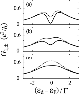
Figure 3: Calculated results of the conductance $G_{1,\pm}$ as a function of energy level, $\varepsilon_{\text{d}}=(\varepsilon_{1}+\varepsilon_{2})/2$, in a three-terminated quantum dot. Solid (broken) lines indicate the conductance $G_{1,+}$ ($G_{1,-}$) for spin $\sigma=+1$ ($-1$). The level broadening by the tunnel coupling to leads S and D$1$ is $\Gamma_{\text{S}}=\Gamma_{\text{D}1}\equiv\Gamma$ ($e_{\text{S},1}/e_{\text{S},2}=1/2$, $e_{\text{D}1,1}/e_{\text{D}1,2}=3$), whereas that to lead D$2$ is (a) $\Gamma_{\text{D}2}=0.2\Gamma$, (b) $0.5\Gamma$, and (c) $\Gamma$ ($e_{\text{D}2,1}/e_{\text{D}2,2}=-1$). $\Delta=\varepsilon_{2}-\varepsilon_{1}=0.5\Gamma$. $\Delta_{\text{SO}}=0.2\Gamma$.

In Fig. 3, the conductance $G_{1,\pm}$ shows a dip at $\varepsilon_{\text{d}}\approx\varepsilon_{\text{F}}$ for small $\Gamma_{\text{D}2}$.[28] Around the dip, the spin polarization is markedly enhanced: $|P|$ is close to unity in panel (a).

Next, we examine the Kondo effect in the Coulomb blockade regime with a single electron in the QD. The Kondo effect is not broken by the SO interaction since the time-reversal symmetry holds. For the electron-electron interaction in the QD, we assume that $H_{\text{int}}=U\sum_{j}n_{j,+}n_{j,-}+U^{\prime}\sum_{\sigma,\sigma^{\prime}}n_{1,\sigma}n_{2,\sigma^{\prime}}$, where $n_{j,\sigma}=d_{j,\sigma}^{\dagger}d_{j,\sigma}$, with infinitely large $U$ and $U^{\prime}$. The Kondo effect creates the many-body resonant state at the Fermi level, and thus condition (ii) is always satisfied. The resonant width is given by the Kondo temperature $T_{\text{K}}$.[29] When $T_{\text{K}}<\Delta$, the upper level in the QD is irrelevant. The spin at the lower level is screened out by the conventional SU(2) Kondo effect. When $T_{\text{K}}>\Delta$, on the other hand, the pseudo-spin as well as the spin are screened by the SU(4) Kondo effect.[30] The latter situation is required for an enhanced SHE since two levels should be relevant to the resonance [condition (i)].

The crossover between the SU(2) and SU(4) Kondo effects can be semiquantitatively described by the slave-boson mean-field theory.[31] The theory describes the Kondo resonant state on the assumption of its presence and Fermi liquid behavior and yields the conductance at temperature $T=0$. A boson operator $b$ is introduced to represent an empty state in the QD. $d_{j,\sigma}^{\dagger}=f_{j,\sigma}^{\dagger}b$ and $d_{j,\sigma}=b^{\dagger}f_{j,\sigma}$, with a fermion operator $f_{j,\sigma}$ representing the pseudo-spin $j$ and spin $\sigma$. $H_{\text{int}}$ is taken into account by the constraint of $Q\equiv\sum_{j,\sigma}f_{j,\sigma}^{\dagger}f_{j,\sigma}+b^{\dagger}b-1=0$. $b$ is replaced with the mean field $\langle b\rangle$, which is determined by minimizing $\langle H+\lambda Q\rangle$ with the Lagrange multiplier $\lambda$.[29] The conductance is given by eq. (15) if $\varepsilon_{\text{d}}$ and $\Gamma_{\alpha}$ are replaced with the renormalized ones, $\varepsilon_{\text{d}}+\lambda$ ($\sim\varepsilon_{\text{F}}$) and $\Gamma_{\alpha}\langle b\rangle^{2}$ ($\sim T_{\text{K}}$), respectively.

Figure 4 shows $G_{1,\pm}$ as a function of $\varepsilon_{\text{d}}$ in the three-terminal system. The parameters are the same as those in the main panels in Fig. 2. In the two-terminal situation (curve $a$; $G_{1,+}=G_{1,-}$), the conductance increases with decreasing $\varepsilon_{\text{d}}$ and saturates, indicating the charge fluctuation regime and Kondo regime, respectively. With three leads (curves $b$–$e$), we observe a spin current around the beginning of the Kondo regime. $P\approx 0.5$ in the case of curve $e$. As $\varepsilon_{\text{d}}$ is decreased further, $T_{\text{K}}$ decreases and becomes smaller than $\Delta$, which weakens the SHE. We obtain similar results using the parameters in Fig. 3.

Figure 4: Calculated results of the conductance $G_{1,\pm}$ as a function of energy level, $\varepsilon_{\text{d}}=(\varepsilon_{1}+\varepsilon_{2})/2$, in a three-terminated quantum dot in the presence of Kondo effect. Solid (broken) lines indicate the conductance $G_{1,+}$ ($G_{1,-}$) for spin $\sigma=+1$ ($-1$). The level broadening by the tunnel coupling to lead D$2$ is $\Gamma_{\text{D}2}=0$ (curve $a$; solid and broken lines are overlapped), $0.2\Gamma$ ($b$), $0.5\Gamma$ ($c$), $\Gamma$ ($d$), and $2\Gamma$ ($e$). The other parameters are the same as those in the main panels in Fig. 2.

In summary, we have examined the SHE in a multiterminated QD with SO interaction. The spin polarization in the output currents is markedly enhanced by resonant tunneling if the level spacing in the QD is smaller than the level broadening. The spin current is also enlarged by the many-body resonance due to the SU(4) Kondo effect. The SHE is electrically tunable by changing the tunnel coupling to the leads.

Hamaya et al. fabricated InAs QDs connected to ferromagnets.[32] If a ferromagnet is used as a source lead in our model, spin filtering is electrically detected through an “inverse SHE.” The current to lead D$1$ is proportional to $(1+p\cos\theta)G_{\text{D}1,+}+(1-p\cos\theta)G_{\text{D}1,-}$, where $p$ is the polarization in the ferromagnet and $\theta$ is the angle between the magnetization and ${\bm{h}}_{\text{SO}}$.

The SHE in QDs is useful for the fundamental research as well as for the application to an efficient spin filter. The SHE enhanced by resonant scattering or Kondo resonance was examined for metallic systems with magnetic impurities.[33, 34, 35] In semiconductor QDs, we can observe the SHE due to the scattering by a single “impurity” with the tuning of various conditions.

The authors acknowledge fruitful discussion with G. Schön and Y. Utsumi. This work was partly supported by a Grant-in-Aid for Scientific Research from the Japan Society for the Promotion of Science, and by the Global COE Program “High-Level Global Cooperation for Leading-Edge Platform on Access Space (C12).” T. Y. is a Research Fellow of the Japan Society for the Promotion of Science.

References

[1]
I. Žutić, J. Fabian, and S. Das Sarma:
Rev. Mod. Phys. 76 (2004) 323.
[2]
E. I. Rashba: Fiz. Tverd. Tela (Leningrad) 2 (1960)
1224 [in Russian].
[3]
Yu. A. Bychkov and E. I. Rashba: J. Phys. C 17
(1984) 6039.
[4]
R. Winkler:
Spin-Orbit Coupling Effects in Two-Dimensional Electron
and Hole Systems (Springer, Heidelberg, 2003).
[5]
J. Nitta, T. Akazaki, H. Takayanagi, and T. Enoki:
Phys. Rev. Lett. 78 (1997) 1335.
[6]
G. Dresselhaus: Phys. Rev. 100 (1955) 580.
[7]
S. Murakami, N. Nagaosa, and S. C. Zhang: Science
301 (2003) 1348.
[8]
J. Wunderlich, B. Kaestner, J. Sinova, and T. Jungwirth:
Phys. Rev. Lett. 94 (2005) 47204.
[9]
J. Sinova, D. Culcer, Q. Niu, N. A. Sinitsyn, T. Jungwirth,
and A. H. MacDonald: Phys. Rev. Lett. 92 (2004) 126603.
[10]
M. I. Dyakonov and V. I. Perel:
Phys. Lett. 35A (1971) 459.
[11]
Y. K. Kato, R. C. Myers, A. C. Gossard, and D. D. Awschalom:
Science 306 (2004) 1910.
[12]
H. Engel, B. I. Halperin, and E. I. Rashba: Phys. Rev. Lett. 95 (2005) 166605.
[13]
M. Eto and T. Yokoyama:
J. Phys. Soc. Jpn. 78 (2009) 073710.
[14]
T. Yokoyama and M. Eto:
Phys. Rev. B 80 (2009) 125311.
[15]
Y. Igarashi, M. Jung, M. Yamamoto, A. Oiwa, T. Machida,
K. Hirakawa, and S. Tarucha:
Phys. Rev. B 76 (2007) 081303(R).
[16]
C. Fasth, A. Fuhrer, L. Samuelson, V. N. Golovach, and D. Loss:
Phys. Rev. Lett. 98 (2007) 266801.
[17]
A. Pfund, I. Shorubalko, K. Ensslin, and R. Leturcq:
Phys. Rev. B 76 (2007) 161308(R).
[18]
S. Takahashi, R. S. Deacon, K. Yoshida, A. Oiwa, K. Shibata,
K. Hirakawa, Y. Tokura, and S. Tarucha:
Phys. Rev. Lett. 104 (2010) 246801.
[19]
A. A. Kiselev and K. W. Kim:
Phys. Rev. B 71 (2005) 153315.
[20]
J. H. Bardarson, I. Adagideli, and Ph. Jacquod:
Phys. Rev. Lett. 98 (2007) 196601.
[21]
J. J. Krich and B. I. Halperin:
Phys. Rev. B 78 (2008) 035338.
[22]
J. J. Krich:
Phys. Rev. B 80 (2009) 245313.
[23]
For ,
is replaced with ,
where , etc.
In InAs QDs, and may coexist.
Then is changed to
.
[24]
Y. Meir and N. S. Wingreen:
Phys. Rev. Lett. 68 (1992) 2512.
[25]
For noninteracting electrons,
and
. The substitution of
these relations into eq. (12) yields
, where
.
[26]
In the presence of more than one channel in a lead,
a spin current can be generated in two-terminal
systems, e.g., see,
M. Eto, T. Hayashi, and Y. Kurotani:
J. Phys. Soc. Jpn. 74 (2005) 1934.
[27]
F. Zhai and H. Q. Xu: Phys. Rev. Lett. 94 (2005) 246601.
[28]
The conductance dip is caused by the destructive
interference between propagating waves through
two orbitals in the QD.
In the two-terminal system without SO interaction,
the conductance
completely vanishes at the dip, where the
“phase lapse” of the transmission phase takes
place. See ref. 36 and related
references cited therein.
[29]
A. C. Hewson: The Kondo Problem to Heavy Fermions
(Cambridge University Press, Cambridge, 1993).
[30]
We have two sets of Kramers’ degenerate levels in the
QD and channels in the leads. By the unitary
transformation for the channels, we obtain
two channels connected to the QD and
channels disconnected from the QD.
This is the situation of the full-screening Kondo
effect.[37]
When , the SU(4) Kondo
effect is realized even when the strengths of the tunnel
coupling are not identical between the two levels in the QD.
This is because the fixed point is marginal (and
thus not unstable) in the Kondo scaling.[38]
[31]
J. S. Lim, M.-S. Choi, M. Y. Choi, R. López,
and R. Aguado:
Phys. Rev. B 74 (2006) 205119.
[32]
K. Hamaya, M. Kitabatake, K. Shibata, M. Jung,
M. Kawamura, K. Hirakawa, T. Machida, T. Taniyama,
S. Ishida, and Y. Arakawa:
Appl. Phys. Lett. 91 (2007) 022107.
[33]
A. Fert and O. Jaoul:
Phys. Rev. Lett. 28 (1972) 303.
[34]
A. Fert, A. Friederich, and A. Hamzic:
J. Magn. Magn. Mater. 24 (1981) 231.
[35]
G. Y. Guo, S. Maekawa, and N. Nagaosa:
Phys. Rev. Lett. 102 (2009) 036401.
[36]
C. Karrasch, T. Hecht, A. Weichselbaum, Y. Oreg,
J. von Delft, and V. Meden:
Phys. Rev. Lett. 98 (2007) 186802.
[37]
P. Nozières and A. Blandin:
J. Phys. (Paris) 41 (1980) 193.