Study of three-dimensional crack fronts under plane stress using a phase field model

Abstract

The shape of a crack front propagating through a thin sample is studied using a phase field model. The model is shown to have a well defined sharp interface limit. The crack front is found to be an ellipse with large axis the width of the sample and small axis a function of the Poisson ratio and the width of the sample. Numerical results also indicate that the front shape is independent of the crack speed and of the sample extension perpendicular to its width.

When a crack grows in an elastic medium under increasing load, one would expect, according to the Linear Elastic Fracture Mechanics (LEFM) theory, that its speed increases and reaches asymptotically the Rayleigh wave speed[1]. Experimentally it has been found that at small loads (and therefore low crack speeds) the theory accounts well for the crack speed. But for higher loads (and for higher crack speeds) the observed phenomena are not predicted by the LEFM. Indeed, above a critical speed that is approximately equal to half the Rayleigh wave speed, the crack speed as a function of time starts to be irregular[2, 3] and the crack surface presents marks indicating the growth of secondary crack branches. The theoretical effort to predict this instability in the framework of the LEFM has not been successful yet even though it has been possible to determine a minimal speed below which the branching can not occur[4, 5]. While experiments have allowed to describe the departure from the LEFM theory they have not been able to give a clear description of the mechanisms leading to the instabilities. This is mainly due to the fact that crack fronts are rapidly moving objects over a long distance compared to the scale at which the instability is assumed to take place (the process zone). In addition to this issue, experiments are limited to the observation of the surface of the sample[3, 6] while it is likely that the instability mechanism occurs in the thickness of the sample[7, 8]. In fact, the theoretical study of propagating cracks has been mostly limited to two dimensional cases and there is no widely accepted law of motion for the crack front in 3D.

Hence, models where the breaking mechanism occuring in the process zone is described in a simplified way are appealing since their use in numerical simulations would gives access to real time observations of the crack front and will hopefully allow to have a better understanding of the branching mechanism. One possible candidate would be the phase field model of crack propagation[9]. It was originally presented in [10] for mode III cracks and then extended to mode I and II[11, 12, 13, 14, 15] and more recently used in the study of the propagation of a tridimensional crack under mixed mode loading[16]. In this model of fracture, elastic energy is converted into surface energy through the evolution of a phase field that governs the elastic constants in the medium (for a review of phase field models of crack propagation see[17]). This approach has the advantages that no law of crack propagation is needed (since the crack propagation is due to the evolution of the phase field) and that, numerically, its implementation is straightforward without the need of any complex interface tracking approach (this is especially advantageous in 3D where surface tracking is involved). Here, after briefly presenting the model and the numerical setup, I present the study of a single crack front propagating through a thin sample under plane stress conditions at its sides(see fig. 1). This work aims at solving a long-standing question dating back to the work of Benthem[18] where it was shown that, contrarily to what is happenning in the quasi two-dimensionnal situation of plane strain, a crack front could not be a straight line in a thin sample since the singularity at the crack front combined with the plane stress condition would lead to infinite displacement in the direction of the front ($z$ direction in fig. 1). Since then, the question of the shape of the crack front has remained unanswered due to the particuliar complexity of the problem involving guessing a law for the crack front motion and computing the interaction of the crack front motion and the elastic field. Here, in the limit of thin samples, the crack front shape (for a given parameter set) is found to be half an ellipse with large axis the thickness of the sample and with small axis a function that is only dependant on the thickness of the sample. It should be noted that it is independant of the crack speed and of the aspect ratio of the sample. When varying the model parameters, the value of the ellipse small axis was found not to depend on the dissipation at the crack tip but to depend on the Poisson ratio of the elastic material. In addition, in the case of thick samples the crack front was no longer found to be an ellipse and its shape was in very good agreement with the prediction of Bazant[19].

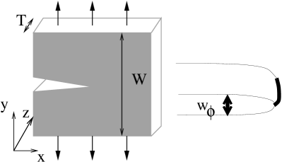
Figure 1: left: axis definition and loading conditions. The boundary conditions are fixed displacement on the top surfaces (xz planes) and either fixed displacement ($u_{z}=0$ plane strain) or zero stress (plane stress) along the z axis on the xy planes. In the case of stable crack propagation, the crack surface is a part of $y=0$ plane and the crack front is the boundary of this part in the y plane. Left Schematic of the isosurface $\phi=0.5$ in the same coordinate system. The crack front is the thick line that corresponds to the most advanced part of the crack surface and is a line in the $y=0$ plane. The crack is propagating from left to right. The isosurface is represented in the material at rest frame. In order to observe the usual parabolic profile in the $z=0$ plane one simply needs to perform the change of coordinates: $x\to x+u_{x}$, $z\to z+u_{z}$, $y\to y+u_{y}$ to take into account the singular strain of the solid at the crack tip.

In the phase field model an additional variable, $\phi$ called the phase field is introduced. It indicates the internal state of the material. The case $\phi=1$ (resp. $\phi=0$) corresponds to an intact (resp. entirely broken) material. The free energy from which the evolution equation of the phase field and of the elastic field derive writes:

$$\mathcal{F} = \iiint dV\frac{w_{\phi}D}{2}(\nabla\phi)^{2}+\frac{1}{w_{\phi}}V_{VDW}(\phi)$$ (1)

$$+ \frac{1}{w_{\phi}}g(\phi)\left(\frac{\lambda}{2}(\mathrm{tr}\epsilon)^{2}+\mu\mathrm{tr}(\epsilon^{2})-\epsilon_{c}^{2}\right)$$

where $\epsilon$ is the symmetric rank 2 strain tensor ($\epsilon_{ij}=(\partial_{i}u_{j}+\partial_{j}u_{i})/2$) with $u_{i}$ the displacement field of the material. The functions are: $V_{DVW}(\phi)=\phi^{2}(1-\phi)^{2}$ and $g(\phi)=4\phi^{3}-3\phi^{4}$. $w_{\phi}$ is a parameter that sets the interface width (which is proportional to $w_{\phi}$) without changing the fracture energy $\gamma=\sqrt{2w_{\phi}D_{\phi}}\int_{0}^{1}d\phi\sqrt{\frac{1}{w_{\phi}}(V_{VDW}+(1-g)\epsilon_{c}^{2})}$[9]. The evolution equation of the displacement field writes:

$$\partial_{tt}u_{i}=-\frac{\delta\mathcal{F}}{\delta u_{i}}$$ (2)

so that, if the phase field is uniformly equal to 1, one retrieves the wave equation for a solid of density 1 and that the region where the phase field is equal to zero cannot transmit any stress. The evolution equation of the phase field is:

$$\tau\partial_{t}\phi=-\frac{\delta\mathcal{F}}{\delta\phi}/\beta$$ (3)

where $\beta$ is a constant kinetic coefficient that measures the dissipation at the crack tip (see [15]) and $\tau$ is a variable kinetic coefficient that is equal to 1 except in the following cases:

• it goes to zero if the r.h.s of eq. 3 is positive, so that the phase field can only decrease (breaking is irreversible).

• $\tau$ is $\max(0,(A+g^{\prime}(\phi)K_{\mbox{Lam\'{e}}}(tr\epsilon)^{2})/A)$ with $A=-\delta\mathcal{F}/\delta\phi$ if $tr\epsilon<0$ so that the compression energy does not contribute to crack growth.

One should note that these kinetic modifier, even if they may prevent the system from reaching a global minimum (in the same way as actual irreversibility does) do not lead to an unphysical increase of the free energy. As previously mentioned these equations have already been used to describe the growth of a crack in a 2D set up. Here I use them to study the crack growth in a 3D set-up considering a plate under plane stress condition

$$\sigma_{xz}=\sigma_{yz}=\sigma_{zz}=0$$ (4)

which translates in:

$$\epsilon_{xz}=0,\,\,\epsilon_{yz}=0\mbox{ and }\epsilon_{zz}=-\lambda*(\epsilon_{xx}+\epsilon_{yy})/(\lambda+2\mu)$$ (5)

with a no-flux boundary condition for the phase field, so that surface terms ($\oiint\delta\phi\mathbf{\nabla}\phi.\mathbf{dS}$) do not contribute to the change in the free energy.

The simulations were performed using finite differences (using a scheme that derives from a discretized free energy) to compute the derivatives and the time stepping was performed using a simple forward Euler scheme. The grid spacing was taken equal to $dx=0.3$ and $dx=0.15$ to check that discretisation effects are negligible.

(a)	(b)
(c)	(d)

Figure 2: (a) and (b)$\bullet$ Points of the crack front computed using the phase field model. The crack is propagating from top to bottom. The line corresponds to the elliptical fit whose large axis is the horizontal line. In (a) a small assymetry of the crack front can be attributed to the use of an asymmetric initial condition. In (b) the crack front has retrieved a symmetric shape after a transient regime. In both cases, the load was $\Delta_{y}=22$, leading to a crack speed of 0.51 the thickness of the sample was: 36 in (a) and 12 in (b) and the width was 160. Poisson ratio here was 0.25. The lack of accuracy of the fit close to the boundary can be attributed to the use of Neuman boundary condition that would impose a crack front perpendicular to the side of the sample while, an ellipse corresponds to a tangential crack front. The effect of the boundary condition is clearer when one considers the slope of the front (c).d For different values of $\beta$ (1, 4, 10, 20, 40 and 80), the value of $e$ is plotted as a function of time during the growth of an accelerating crack. Poisson ratio is 0,25 and the width of the sample is 24. In the inset, the behavior of $e$ as a function of the distance travelled by the crack is shown for $\beta$ equal to 20, 40 and 80.

In this model, the crack surface can be seen as the $\phi=0.5$ iso surface and the coordinate system is the elastic body at rest. Hence, the crack surface in the $x0y$ plane corresponds to a single thin finger using the present coordinate system. To retrieve the laboratory frame, one needs to apply the coordinate change:$x\leadsto x+u_{x}(x,y,z),\ y\leadsto y+u_{y}(x,y,z),\ z\leadsto z+u_{z}(x,y,z)$. Using this coordinate change, one retrieves the parabolic crack front opening far from the tip (see [20] for the effects of a non-linear elastic zone at the crack tip). The crack front was taken as the set of points of higher $x$ of the isoline $\phi=0.5$ in each $x0y$ plane (see fig 1) and it was a line in the $y=0$ plane.

Numerical simulations showed that in the case of a single crack the points were located at the middle of the sample ($y=0$). While the crack front reached a steady shape after a transient regime when the crack speed was below the branching threshold, in the quantitative study an averaging procedure (usually over 5 to 10 snapshots of the front equally spaced in time) was used to reduce the discretisation effects.

Figure 3: left: For a given parameter set and two distinct thickness of the sample $e$ as a function of $w_{\phi}$ in space units, the interface thickness. . The $+$ and $\times$ correspond to $T=12$ and $W=80$ and $320$. One can see that in both cases there is convergence toward a well defined limit that does not depend on $W$. The $*$ symbol corresponds to $T=24$ and $W=320$. There is also a well defined convergence. The lines serve as a guide to the eye. right: shape of half the crack front in the case where $T/W$ is of order unity (3.4). One can see that it is roughly V-shaped and that the angle made by the crack front with the free boundary in $z=0$ is roughly $0.557\pi$ (angle made by the dashed line), to compare with the value of $\approx 0.546\pi$ in fig 10. of [19].

Results are discussed as follows. First, the shape of the crack front in the case of thin samples is described. Then the dependence of the crack front on the phase field interface thickness is discussed from a quantitative point of view and the model is shown to converge toward a well defined limit when the interface thickness is decreased toward 0. Finally, the dependence of the crack front on relevant physical parameters is discussed. The physical parameters considered here are the geometry of the sample: that is the ratio $T/W$ and the actual value of $T$, the poisson ratio of the material $\nu=\lambda/(2(\lambda+\mu)$, the load applied to the material that is directly related to the crack speed and the kinetic coefficient $\beta$ that governs dissipation at the crack tip.

Before describing the crack front, the change in crack speed is briefly discussed. When considering a single crack propagating in a thin plate (the quantitative meaning of thin will be precised later), one expects to retrieve the results one would get from a 2D computation. Indeed, in both cases, the crack propagation can be described as transforming elastic energy stored in the material at rest into kinetic energy (in elastic waves) and surface energy. Only a little slow down of the crack due to the additional degree of freedom along the z axis (along which elastic wave will also propagate) is expected. Simulations have shown that this is the case and that there is very little difference between the speed computed using 3D simulations and the speed computed using 2D simulations provided the elastic coefficients are rescaled to take into account the zero stress condition.

Figure 4: left: The ratio $e$ of small axis of the crack front ellipse $eW$ on the sample width $W$ is plotted as a function of the Poisson ratio $\nu$. The phase field parameters are kept unchanged. For a given value of Poisson ratio $e$ is taken as the average of a few simulations where the load (and as a result the crack speed) was varied. The variation of $e$ across these simulations, for a given value of $\nu$ was less than 5% and no clear trend when varying the load could be identified. right: $e$ is plotted as a function of the sample width for two different values of its extension along y (160 and 320) for a value of the poison ratio of 0.25.

As already shown([19]) the zero-stress condition implies that the crack front cannot be flat. Numerical results show that this is actually the case and the crack front is not flat and presents a noticeable curvature at its tip. A fit of the crack front using various possible test functions (such as power laws) indicated that the best fit is an ellipse with large axis the half thickness of the sample $T/2$ and small axis $eT$ where $e$ is a real constant. (see fig.2). The equation of the ellipse in the following will write:

$$1=\frac{z^{2}}{(T/2)^{2}}+\frac{x^{2}}{(Te)^{2}}.\ y=0$$ (6)

It should be noted here that since $T$ is fixed, there is only one adjustable parameter for the fit: $e$ which is a priori a function of other parameters describing the system (load, elastic constants and geometry of the sample). This fit was valid only for thin samples where $W/T$ was approximately larger than 5. For thicker samples the crack front was no longer elliptical and its shape will be briefly discussed here. I now turn to the convergence of the model, that is the role of the interface thickness $w_{\phi}$.

In phase-field simulations, the role of the interface thickness has to be measured and one needs to show that a proper sharp interface limit exists when the interface thickness goes to zero keeping other parameters constant (including the surface energy). In our model, this can be done by varying $w_{\phi}$ and one can easily show that the interface thickness is proportional to $w_{\phi}$ while the surface energy is kept unchanged[9]. Simulations using various values of $w_{\phi}$ (namely 1,2,3 and 4) have shown that the value of $e$ converges toward a well-defined limit when $w_{\phi}$ goes to 0 (see fig. 3). Moreover, they show that the relative error made when considering the case $w_{\phi}=1$ is of the order $10\%$. This indicates that the model has a well defined limit when $w_{\phi}$ is decreased toward 0. One should note that when $w_{\phi}$ is decreased both the phase field interface thickness and the phase field process zone size are going toward zero and that the model has not a well defined sharp interface limit as solidification models do. Nevertheless, the fact that the size of the process zone decreases proportionnally to the interface thickness is coherent with the LEFM theory where the process zone is a point. In the following all the results considered were obtained using $w_{\phi}=1$.

Figure 5: (a) and (b) Successive snapshots of the iso surface $\phi=0.5$ taken during a branching event under plane stress condition (more precisely those are juxtaposed isolines taken in each $z=i\ dx$ plane. The whole simulation domain is not shown.). One can see that the branches are appearing at the middle of the sample and spreading toward the sides of the sample. The crack is propagating toward us along the arrow. In (c), one can see the branching event shown in (b) from behind and the typical shape of the sidebranches that is similar to the branches observed in [21]. The schematic axis at bottom correspond to (c).

I now turn to the study of the dependence of $e$ on the different parameters characterizing the physical system. First a system where the geometry ($W$ and $T$) , the elastic constants ($\lambda,\ \mu$ and more importantly $\nu$) and the fracture energy are fixed while the crack speed is varied is considered. The variation in the crack speed can be achieved either by changing the load or by changing the dissipation ($\beta$) at the crack tip. As can be seen in fig.2 d, changing the value of $\beta$ does not affect significantly $e$. Varying the load did not change the value of $e$ for a wide range of crack speeds (0.05 $c_{s}$ to 0.4 $c_{s}$, close to the threshold speed at which the branching instability occurs ).

In the following, the effects of the parameters describing the mechanical problem (i.e. the Poisson ratio and the geometry of the sample.) are investigated.

First for a given geometry sample (fixed $T$ and $W$), the value of the Poisson ration $\nu$ was varied (by changing $\lambda$ and $\mu$). As shown in fig. 4 the value of $e$ is significantly affected by the Poisson ratio. For small values of $\nu$, the value of $e$ is small and the crack front is almost flat as it is expected in the plane strain situation. This is not surprising since for $\nu$ close to zero, the amplitude of the so-called Poisson effect is small and the difference between plane stress and plane strain condition is small. More precisely, in the limit where $\nu$ goes to zero, one expects the plane stress and plane strain condition to be equivalent and therefore the crack front is expected to be flat. Here, the limit of $e$ when $\nu$ goes to zero is zero which is in agreement with this prediction.

On the opposite for values of $\nu$ close to 0.5 (incompressible limit), the value of $e$ is much higher and goes toward a finite limit when $\nu$ goes to $0.5$ (its maximal value corresponding to an incompressible material where the difference between the plane strain and plane stress condition should be the highest).

Now I turn to the description of the effects of the sample geometry. All results were obtained for a given Poisson ratio $\nu=0.25$ and, in the case of thin samples, various values of the width $W$ (80, 160 and 320 space units (su)) and thickness $T$ (from 6 to 60 su) of the sample. The value of the width of the crack $w_{\phi}$ was kept constant. In the case of thick samples, values of $T$ equal to $W$ and larger were used. First the results obtained using thin samples are presented. In this situation, $T\ll W$, the crack front is half an ellipse and it is completely described by the value of $e$. In this situation, it appears that $e$ is a function of $T$ and does not depend on $W$ as can be seen on fig. 4 where the computed values of $e$ are plotted as a function of $T$ for two different values of $W$ (160 and 320 su) and collapse well on a master curve. When $T$ goes to zero, one can see that $e$ converges toward a well defined finite limit. When $T$ goes to infinity, the behaviour of $e$ is still not clear since the present data do not allow to determine wether it converges toward a finite limit or wether it decreases toward 0.

When considering thick samples, the use of $u_{z}=u_{x}=0$ as top and bottom boundary conditions leads to the fact that most of the elastic material is under plane strain. Then the system is in a situation where the work of Bazant[19] can be applied. As a result one expects the crack front to intersect the free boundary with a finite angle that is a function of the Poisson ratio. Numerical results are in good agreement with this prediction. Indeed, as can be seen in fig. 3 where half the crack front is plotted, the crack front is V-shaped and intersects the free boundary with a finite angle. Moreover, the value of the angle obtained during numerical simulations is a function of the Poisson ratio and is in good agreement with the prediction of [19].

Hence, this work indicates that the shape of a crack front through a thin sample is half an ellipse that is tangent to its sides. The small axis of this ellipse is, as one would have expected, a function of the Poisson ratio of the material and, more surprisingly, of the thickness of the sample, independantly of its width. Extensive checks on parameters show that the dependance on other parameters of the crack front propagation is not significant. Indeed, simulations have shown that the crack front shape is independant of the crack speed, the dissipation at the crack tip and the width of the sample (provided one stays in the $T\ll W$ regime). In addition, the behaviour of the model was checked against predictions made using the LEFM theory in the case of thick samples[19] and a good agreement was found.

This study stresses one of the main interest of the phase-field modelling of crack propagation in three dimensions: it allows to predict the shape of a crack front without any a priori hypothesis.

Another continuation of this work would be to use the phase field model to understand the branching instability in three dimensions. Indeed, from a qualitative point of view, the phase field model allows to reproduce well three dimensionnal branching events (see fig. 5) with a good qualitative agreement with experimental findings[21] as far as the shape of the branch is concerned.