Detectability of Orbital Motion in Stellar Binary and Planetary Microlenses

Abstract

A standard binary microlensing event lightcurve allows just two parameters of the lensing system to be measured: the mass ratio of the companion to its host, and the projected separation of the components in units of the Einstein radius. However, other exotic effects can provide more information about the lensing system. Orbital motion in the lens is one such effect, which if detected, can be used to constrain the physical properties of the lens. To determine the fraction of binary lens lightcurves affected by orbital motion (the detection efficiency) we simulate lightcurves of orbiting binary star and star-planet (planetary) lenses and simulate the continuous, high-cadence photometric monitoring that will be conducted by the next generation of microlensing surveys that are beginning to enter operation. The effect of orbital motion is measured by fitting simulated lightcurve data with standard static binary microlensing models; lightcurves that are poorly fit by these models are considered to be detections of orbital motion. We correct for systematic false positive detections by also fitting the lightcurves of static binary lenses. For a continuous monitoring survey without intensive follow-up of high magnification events, we find the orbital motion detection efficiency for planetary events with caustic crossings to be $0.061\pm 0.010$, consistent with observational results, and $0.0130\pm 0.0055$ for events without caustic crossings (smooth events). Similarly for stellar binaries, the orbital motion detection efficiency is $0.098\pm 0.011$ for events with caustic crossings and is $0.048\pm 0.006$ for smooth events. These result in combined (caustic crossing and smooth) orbital motion detection efficiencies of $0.029\pm 0.005$ for planetary lenses and $0.070\pm 0.006$ for stellar binary lenses. We also investigate how various microlensing parameters affect the orbital motion detectability. We find that the orbital motion detection efficiency increases as the binary mass ratio and event time-scale increase, and as impact parameter and lens distance decrease. For planetary caustic crossing events, the detection efficiency is highest at relatively large values of semimajor axis $\sim 4$ AU, due to the large size of the resonant caustic at this orbital separation. Effects due to the orbital inclination are small and appear to only significantly affect smooth stellar binary events. We find that, as suggested by Gaudi (2009), many of the events that show orbital motion can be classified into one of two classes. The first class, separational events, typically show large effects due to subtle changes in resonant caustics, caused by changes in the projected binary separation. The second class, rotational events, typically show much smaller effects, which are due to the magnification patterns of close lenses exhibiting large changes in angular orientation over the course of an event; these changes typically cause only subtle changes to the lightcurve.

1 Introduction

The current gravitational microlensing surveys, OGLE (Udalski, 2003) and MOA (Hearnshaw et al., 2005) discover $\sim 700$ unique microlensing events per year, of which, of order ten percent show signatures of lens binarity. A small fraction of these, those with a high probability of planet detection, are followed-up by a number of follow-up teams, which intensively monitor the events for the signatures of planets. In the coming years this strategy will be augmented and extended by a strategy of continuous, high cadence surveys, performed by a global network of wide field telescopes. Such a network will monitor all the microlensing events it discovers with a cadence similar to that achieved by the follow-up networks for a handful of events today.

The lightcurve of a standard static binary lens, in which the lens components are fixed and the source follows a straight path, can be described by a minimum of seven parameters. Only three of these parameters contain physical information about the lens system. Two are dimensionless parameters: the mass ratio $q$, and the projected separation of the lens components $d$, measured in units of the Einstein radius. The third, the Einstein time-scale of the event $t_{\mathrm{E}}$, is the time taken for the source to cross one Einstein radius

$$t_{\mathrm{E}}=\frac{r_{\mathrm{E}}}{v_{\mathrm{t}}},$$ (1)

where $v_{\mathrm{t}}$ is the relative projected lens-source velocity and $r_{\mathrm{E}}$ is the Einstein radius. This is defined as

$$r_{\mathrm{E}}=\sqrt{\frac{4G}{c^{2}}x(1-x)D_{\mathrm{s}}M},$$ (2)

where $x=D_{\mathrm{l}}/D_{\mathrm{s}}$ is the ratio of the lens distance $D_{\mathrm{l}}$ to the source distance $D_{\mathrm{s}}$ and $M$ is the total mass of the binary. Of the other four parameters, three are purely geometrical, and the final parameter is the unlensed source flux.

The mass ratio and separation are closely related to the most interesting properties of the binary, the component masses and the semimajor axis of the orbit. They can be measured very accurately from a lightcurve, but only describe the binary’s properties in terms of ratios relative to the typical physical scales of the system. The Einstein crossing time-scale $t_{\mathrm{E}}$ contains information on these scales, but this information is wrapped up in a three-fold degeneracy (the so-called microlensing degeneracy) between the total binary mass, the lens distance and the source velocity. It is also dependent on the source distance, but this is usually well constrained by measurements of the baseline flux. To gain any more knowledge of the lens system requires that this degeneracy be broken, either by the detection of higher order effects in the event lightcurve, or by detection of the lens flux and proper motion as the lens and source separate. These detections yield measurements of the lens distance and source velocity respectively, allowing the lens mass to be solved for (Gould & Loeb, 1992; Bennett et al., 2006). Higher order effects, such as finite source effects (Witt & Mao, 1994; Nemiroff & Wickramasinghe, 1994; Alcock et al., 1997) and microlensing parallax (Refsdal, 1966; Gould, 1992; Alcock et al., 1995), allow the microlensing degeneracy to be broken or reduced through measurement or constraint of some of the parameters that are combined in $t_{\mathrm{E}}$. For example detections of finite source effects and microlensing parallax in the same event yield two independent measurements of the angular Einstein radius $\theta_{\mathrm{E}}=r_{\mathrm{E}}/D_{\mathrm{l}}$, which allow the source velocity and lens distance to be eliminated, and the lens mass determined (e.g. An & Gould, 2001).

Orbital motion of the binary lens is another such higher order effect. If the binary lens components are gravitationally bound, they will orbit each other, and their projected orientation will change as a microlensing event progresses. As the magnification pattern produced by a binary lens is not rotationally symmetric, the change in orientation may be detectable in the lightcurve of the event. If the orbit is inclined relative to the line of sight, then the projected separation of the lens components will also evolve, causing changes in the structure of the magnification pattern, which again may be detectable. In a small fraction of binary microlensing events we can expect to see the effects of this orbital motion in their lightcurves, though this is the first work that attempts to quantify this fraction. If orbital motion can be detected in a microlens it can provide constraints on the mass of the lens, and information about the binary orbit.

To date, six binary microlensing events have shown strong evidence of orbital motion in the lens system. The first, MACHO-97-BLG-41 was a stellar mass binary. Modelling of the event was only able to measure the change in the projected angle and separation of the binary in the time between two caustic encounters, but was unable to constrain the orbital parameters (Albrow et al., 2000). The second event, EROS-BLG-2000-5, had very good lightcurve coverage, which allowed the measurement of the rates of change of the binary’s projected separation and angle; these measurements were then used to obtain a lower limit of the orbit’s semimajor axis and an upper limit on the combined effect of inclination and eccentricity (An et al., 2002). The third and fourth examples, OGLE-2003-BLG-267 and OGLE-2003-BLG-291 both seem to show orbital motion effects (Jaroszynski et al., 2005). However, only OGLE survey data was used in their analysis, without follow-up measurements, so the lightcurve coverage was not ideal. Combined with parallax measurement, the masses of both binary lenses were constrained, but no constraints could be placed on the orbits (Jaroszynski et al., 2005). In each of these four cases, the ratio of the component masses is large (near unity), indicative of the lens systems being binary stars, however, orbital motion has recently been measured in two events involving planetary mass secondaries. After the paper was submitted, two further events have been shown to display orbital motion effects: OGLE-2005-BLG-153 (Hwang et al., 2010) and OGLE-2009-BLG-092/MOA-2009-BLG-137 (Ryu et al., 2010).

OGLE-2006-BLG-109 was an event involving a triple lens, with analogues of Jupiter and Saturn orbiting a $\sim 0.5M_{\sun}$ star (Gaudi et al., 2008). The lightcurve of the event had extremely good coverage, and showed multiple features, allowing the orbital motion of the Saturn analogue to be detected. The detection was so strong that the semimajor axes of both planets could be strongly constrained (Gaudi et al., 2008). A more complete analysis of the event, incorporating measurements of the lens flux and orbital stability constraints, carried out by Bennett et al. (2010), tightly constrained four out of six Keplerian orbital parameters of the Saturn analogue, and weakly constrained a fifth. The planet OGLE-2005-BLG-071Lb is a $\sim 4$ Jupiter mass planet orbiting a $\sim 0.5M_{\sun}$ star (Udalski et al., 2005). Measurements of the orbital motion in this event have allowed some constraints to be placed on the planet’s orbit (Dong et al., 2009). In all six events other higher order effects have also been detected, most notably microlens parallax and finite source effects, which are detected in all the events, and in each case allow the measurement of the lens mass.

Despite these detections, there has been relatively little theoretical work on orbital motion in microlensing, likely due to the traditional assumption that the effects of orbital motion on a binary microlens lightcurve will be small and in most cases negligible (e.g. Mao & Paczyński, 1991). The problem was first considered in detail by Dominik (1998), who concluded that in most microlensing events the effects of lens orbital motion were likely to be small, though in some cases lightcurves could be dramatically different. Dominik (1998) points out that the effect is most likely to be seen in long duration binary microlensing events with small projected binary separations. Ioka, Nishi & Kan-Ya (1999) also studied the problem, and pointed out that the effect of binary lens rotation is likely to be important in self-lensing events in the Magellanic clouds. Rattenbury et al. (2002) showed that orbital motion could affect the planetary signatures seen in high-magnification events.

The six microlensing events that display orbital motion make up a significant fraction of the few tens of binary microlensing events that have been modelled (e.g. Alcock et al., 2000; Jaroszynski, 2002; Jaroszynski et al., 2004, 2006; Skowron et al., 2007), which begins to shed doubt on the previous conclusion that lens orbital motion is likely to be unimportant in most binary events. The two planetary events constitute approximately 15 percent of the entire published microlensing planet population. These observations motivate us to revisit the question: how likely are we to see lens orbital motion in a microlensing event? This question is made especially pertinent in the context of the next generation of high cadence microlensing surveys which will make the exquisite lightcurve coverage of EROS-BLG-2000-5 and OGLE-2006-BLG-109 the norm rather than the exception. To gain a better understanding of how frequently orbital motion affects microlensing lightcurves we simulate a large number of microlensing events caused by orbiting binary lenses. We also investigate the factors that affect this frequency.

The structure of the work is as follows. In Section 2 we will review the basic theory of binary microlensing, and the effects of orbital motion on such lensing systems. Section 3 describes our simulations of microlensing events and Section 4 describes how we measure the effects of orbital motion. In Section 5 we present the results of the simulations. We discuss the results in Section 6 and conclude in Section 7.

2 Microlensing with orbiting binaries

2.1 Binary microlensing

The lens equation of a binary point mass gravitational lens describes the mapping of light rays from the source plane to the image plane, and can be written in complex form (Witt, 1990)

$$z_{\mathrm{s}}=z-\frac{1}{1+q}\left(\frac{1}{\overline{z}-\overline{z}_{\mathrm{1}}}+\frac{q}{\overline{z}-\overline{z}_{\mathrm{2}}}\right)$$ (3)

where $z_{\mathrm{s}}=x_{\mathrm{s}}+iy_{\mathrm{s}}$ is the complex coordinate in the source plane, $z=x+iy$ is the complex coordinate in the image plane, $q\leq 1$ is the mass ratio of the secondary mass to the primary, $z_{\mathrm{1}}=x_{\mathrm{1}}+iy_{\mathrm{1}}$ and $z_{\mathrm{2}}=x_{\mathrm{2}}+iy_{\mathrm{2}}$ are the complex coordinates of the primary and secondary lens respectively, and bars represent complex conjugation. All lengths have been normalized to the Einstein radius of the total lensing mass. The positions of the images $z$ for a given source position are found by solving this equation, which can be rearranged into a fifth-order complex polynomial in $z$. The total magnification of the images is given by the ratio of image areas to the source area. This information is contained in the Jacobian of the lens mapping $J$, and the magnification is given by

$$A=\frac{1}{\det J},$$ (4)

where $\det J$ is the determinant of the Jacobian and is given by

$$\det J=1-\left|\frac{1}{1+q}\left(\frac{1}{(\overline{z}-\overline{z}_{\mathrm{1}})^{2}}+\frac{q}{(\overline{z}-\overline{z}_{\mathrm{2}})^{2}}\right)\right|^{2}.$$ (5)

It is possible for $\det J$ to be zero; if this occurs, the magnification of a point source will be infinite at the point in the source plane where $\det J=0$. This occurs when the quantity within the modulus sign in equation (5) lies on the unit circle in the Argand diagram. Any point in the image plane that obeys $\det J=0$ is a critical point. The set of critical points form a set of closed curves called critical curves. The critical curves can be found by solving the critical curve equation

$$\frac{1}{\left(z-z_{\mathrm{1}}\right)^{2}}+\frac{q}{\left(z-z_{\mathrm{2}}\right)^{2}}=(1+q)e^{i\phi}$$ (6)

where $\phi$ is a parameter, such that when swept over $0\leq\phi<2\pi$, the solutions $z$ draw out the critical curves. These can then be mapped through the lens equation (3) onto the source plane to form caustics. A point source that lies on such a caustic will be infinitely magnified, but this unphysical magnification remains finite for physical, finite sources. The caustics are characteristically made up of smooth curves, fold caustics, that meet at cusps.

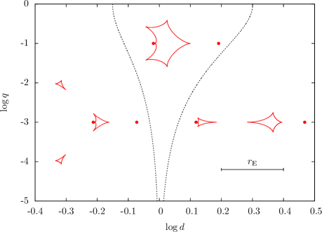
Figure 1: Plot showing the $d$-$q$ plane separated into three regions where the caustics take on close, resonant and wide topologies, with increasing $d$; the dashed lines, $d_{\mathrm{c}}(q)$ and $d_{\mathrm{w}}(q)$, separate the regions of different topology. The solid lines are examples of each of the caustic topologies, drawn to the same scale, for a binary lens with $q=0.1$, and $d=0.7$ (close), $d=1.05$ (resonant) and $d=1.75$ (wide). The filled circles show the positions of the lenses for each topology, with the primary (more massive) lens being positioned leftmost in all cases. After Cassan (2008).

The number and shape of caustics is determined by just two lens parameters, the mass ratio $q$ and the projected lens separation $d$ in units of Einstein radii. There are three possible topologies that the caustics can assume: close, resonant and wide; examples of each are shown in Figure 1. The lines that delimit the different topologies in the $(d,q)$ plane, also shown in the figure, are given by Erdl & Schneider (1993):

$$d_{\mathrm{c}}^{8}=\frac{(1+q)^{2}}{27q}(1-d_{\mathrm{c}}^{4})^{3},$$ (7)

which separates regions of close and resonant topology, and

$$d_{\mathrm{w}}^{2}=\frac{(1+q^{\frac{1}{3}})^{3}}{1+q},$$ (8)

which separates regions of resonant and wide topology.

2.2 Orbital motion in a binary microlens

The lightcurve of a microlensing event can be considered as a one-dimensional probe, by the source, of the two-dimensional magnification pattern produced by the lens. The magnification pattern of a single lens is rotationally symmetric about the position of the lens, but the magnification pattern of a binary lens is more complicated, containing strong caustic structures that exhibit a reflectional symmetry about the binary axis, the axis connecting the lens components. However, far away from the caustics, the magnification pattern can resemble that of a single lens.

As the lens components orbit each other, their position angle and their projected separation can change. These changes cause changes in the orientation and structure of the magnification pattern respectively. It is clear, however, that only if the source traverses regions of the magnification pattern that differ significantly from that of a single lens, will it be possible to detect these effects of orbital motion. For the effects to be measurable the lightcurve of the event must be affected in a significant way, that is not reproducible by a static binary lens model. It is also possible to detect the effect of orbital motion by showing that a static model is less physically plausible than an orbiting model, but this will usually require further information about the event, such as an independent constraint on the lens mass.

The effects of orbital motion on a lightcurve can also be mimicked by other higher order effects, especially parallax and xallarap. Parallax effects are caused by the motion of the earth about the sun, and cause the source to take an apparently curved path through the magnification pattern (e.g. Smith, Mao & Paczyński, 2003). In the case of xallarap, the source travels along a curved path through the magnification pattern as a result of binary orbital motion in the source system (Griest & Hu, 1992; Paczynski, 1997; Dominik, 1998; Rahvar & Dominik, 2009). These curved paths can look very similar to those taken by the source in the rotating binary lens centre of mass frame, and hence it can sometimes be difficult to identify the true cause of the effect.

3 Simulating a high cadence microlensing survey

The major aims of this study are two-fold: firstly to determine the fraction of microlensing events that will be affected by orbital motion, as seen by the next generation microlensing surveys; and secondly, to investigate the factors that affect the detectability of orbital motion, to aid the targeting of such events without resorting to exhaustive modelling efforts. To achieve the first goal, the various factors that go into the observation of a microlensing event should be simulated, accurately modelling the observing setup, the distributions of planetary and binary star lens systems, and the distribution of the sources and lenses throughout the Galaxy. To achieve the second goal we must simplify the parameter space we investigate as far as possible, without removing essential elements from the model, so as to allow a clear interpretation of the results.

To balance these somewhat contradictory requirements we choose to accurately simulate ideal photometry and use a semi-realistic model of the Galaxy, while investigating a logarithmic distribution of companion masses and separations. This allows us to use our simulations to gain a good order of magnitude estimate of the results expected from future surveys, whilst simultaneously investigating the factors that have the largest impact on the detection of orbital motion over a relatively uniform parameter space.

3.1 The Galactic model

To simulate the kinematic and distance distributions of the source and lens populations we assume a simplistic bulge and disk model of the Galaxy. We assume the source to be located in the bulge, at a fixed distance $D_{\mathrm{s}}=R_{\mathrm{0}}=8$ kpc, in the direction of Baade’s Window, where $R_{\mathrm{0}}$ is the distance to the Galactic centre. The lens distances are distributed according to the stellar density distribution of Model II of Binney & Tremaine (2008), which consists of a thin and a thick exponential disk and an oblate spheroidal bulge with a truncated power-law density distribution. The kinematics of our Galactic model are based on that of Han & Gould (1995b), who describe the kinematics of a stellar disk and a barred bulge. The distribution of relative source velocities $\mathrm{d}n/\mathrm{d}v_{\mathrm{t}}$ is dependent on the transverse velocities of the lens, source and observer, and their corresponding velocity distributions. The observer is assumed to follow the Galactic rotation at the position of the Sun, and therefore has a velocity $(v_{\mathrm{O},\ell},v_{\mathrm{O},b})=(225.2,7.2)$ km s^-1 in the directions of Galactic coordinates $(\ell,b)$, once the Solar apex motion is included. The source and lens are assumed to follow the Galactic rotation, with an additional random component. Their velocities have the form, in the directions $\ell$ and $b$,

$$v_{\ell}=v_{\mathrm{rot}}+v_{\mathrm{rand},\ell}\text{, }v_{b}=v_{\mathrm{rand},b},$$ (9)

where $v_{\mathrm{rot}}$ is the rotational component of the velocity, and $v_{\mathrm{rand},\ell}$ and $v_{\mathrm{rand},b}$ are random velocities in the directions $\ell$ and $b$ respectively. The rotation curve of the bulge is assumed to be flat beyond a distance of $1$ kpc from the Galactic centre, and that of a solid body within $1$ kpc. Therefore, the rotational velocity component $v_{\mathrm{rot}}$ for bulge stars is

$$v_{\mathrm{rot}}=\left\{\begin{array}[]{c}v_{\mathrm{max}}\left(\frac{R}{\text{kpc}}\right)\text{ if }R<1\text{ kpc}\\ v_{\mathrm{max}}\text{ if }R\geq 1\text{ kpc}\end{array}\right.$$ (10)

where $v_{\mathrm{max}}=100\text{~{}km~{}s}^{-1}$ is the maximum rotational velocity of the bulge, and $R=\sqrt{X^{2}+Y^{2}}$ and $(X,Y,Z)$ is a galactocentric coordinate system with the $X$-axis increasing towards the observer and the $Z$-axis pointing out of the Galactic plane; for the disk $v_{\mathrm{rot}}=200\text{~{}km~{}s}^{-1}$. The random velocity components are assumed to follow Gaussian distributions, with dispersions taken from Han & Gould (1995a). These dispersions are $(\sigma_{\ell},\sigma_{b})=(30,20)\text{~{}km~{}s}^{-1}$ for the disk and $(\sigma_{X},\sigma_{Y},\sigma_{Z})=(110,82.5,66.3)\text{~{}km~{}s}^{-1}$ for the bulge. From these quantities, the relative transverse velocity of the source $v_{\mathrm{t}}$ (the quantity we are interested in) can be calculated from the relative velocities in the $\ell$ and $b$ directions $v_{\ell}$ and $v_{b}$ as

$$v_{\mathrm{t}}=\sqrt{v_{\ell}^{2}+v_{b}^{2}},$$ (11)

where (e.g. Han & Gould, 1995b)

$$v_{\ell,b}=(v_{\mathrm{l}}-v_{\mathrm{o}})_{\ell,b}+x(v_{\mathrm{o}}-v_{\mathrm{s}})_{\ell,b},$$ (12)

and $v_{\mathrm{o}},v_{\mathrm{l}}$ and $v_{\mathrm{s}}$ are the observer, lens and source velocities respectively, in the directions $\ell$ and $b$.

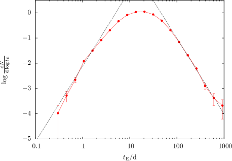
Figure 2: The Einstein time-scale distribution for $\sim 50000$ simulated events. The solid line and data points show the simulated data, and the dashed lines show lines of slope $3$ and $-3$, the expected asymptotic behaviour of the distribution.

The final distribution of lens distances and velocities takes into account the dependence of the event rate $\Gamma\propto\sqrt{x(1-x)}v_{\mathrm{t}}$ on the distribution of each parameter. While the kinematic and density distributions are produced from different Galactic models, they qualitatively reproduce the observed Einstein crossing time-scale distribution, shown in Figure 2, including its asymptotic behaviour (Mao & Paczyński, 1996).

3.2 The microlensing events

When observing a microlensing event, it is often the case that the light of the source being magnified is blended with that of nearby stars in the field. The amount of blending can be quantified by a blending fraction $f_{s}$, which we define to be the fraction of the total flux of the observed blend that the source contributes when unmagnified, such that the time dependent magnitude of the blend is

$$I(t)=I_{\mathrm{b}}-2.5\log(f_{s}A(t)+(1-f_{s})),$$ (13)

where $I_{\mathrm{b}}$ is the baseline magnitude of the observed blend when the source is unmagnified, and $A(t)$ is the magnification caused by the lens.

The distribution of baseline magnitudes and blending fractions is drawn from simulations of blending effects by Smith et al. (2007), who perform photometry on mock images of typical Galactic bulge fields with high stellar density. Specifically we calculate the blending fraction and baseline magnitude for each event from the input and output magnitudes of source stars drawn from their simulation with $1.05$ arcsec seeing and input stellar density of $133.1$ stars arcmin^-2, before any detection efficiency cuts are made to the catalogue. As the phenomenon of negative blending, the source apparently contributing a fraction $f_{s}>1$ to the total flux of the blend (Park et al., 2004; Smith et al., 2007), is poorly understood, we only include sources with moderate negative blending, requiring that $f_{s}<1.2$.

The mock images are produced by Smith et al. (2007) using the method of Sumi et al. (2006), drawing stars from the Hubble Space Telescope $I$-band luminosity function of Holtzman et al. (1998), adjusted to account for denser fields and brighter stars using OGLE data. Extinction was accounted for using the extinction maps of Sumi (2004), and the baseline magnitudes were measured using the standard OGLE pipeline based on dophot (Schechter et al., 1993). Further details can be found in section 3 of the Smith et al. (2007) paper, and references therein.

The lens systems are composed of a primary of mass $M_{\mathrm{1}}$, and secondary of mass $M_{\mathrm{2}}$. The primary’s mass is drawn from a broken power-law distribution

$$\frac{\mathrm{d}n}{\mathrm{d}M_{\mathrm{1}}}\propto M_{\mathrm{1}}^{(\alpha+0.5)};\text{ }\alpha=\left\{\begin{array}[]{cr}-1.3&M_{\mathrm{1}}\leq M_{\mathrm{break}}\\ -2.0&M_{\mathrm{1}}>M_{\mathrm{break}}\end{array}\right.,$$ (14)

with lower and upper limits of $0.05M_{\sun}$ and $1.2M_{\sun}$ respectively, and where $M_{\mathrm{break}}=0.5M_{\sun}$. The addition of $0.5$ to the power-law index is to account for the dependence of the microlensing event rate on the mass of the lens. We do not include a population of stellar remnant lenses, such as white dwarfs, neutron stars and black holes. The mass ratio $q$ of the secondary to the primary is drawn from a logarithmic distribution, with limits $10^{-2}\leq q<1$ for stellar binary lenses and $10^{-5}\leq q<10^{-2}$ for planetary lenses. Note that for lower mass primaries, the distribution of stellar binary mass ratios does include secondaries with masses as low as $\sim 5M_{\mathrm{Jupiter}}$, well into the planetary mass regime, and the lower limit of the planetary mass ratio distribution implies a secondary of $\sim 1M_{\earth}$ for a $0.3M_{\sun}$ primary.

The components of the lens orbit their combined centre of mass in Keplerian orbits, of semimajor axis $a$, distributed logarithmically over the range $0.1\text{AU}\leq a<20\text{AU}$. These orbits are inclined to the line of sight, with inclination angles distributed uniformly over a sphere. For binary stars we performed two sets of simulations, one with zero eccentricity $e$, and another with bound, eccentric orbits with eccentricities distributed uniformly over $0\leq e<1$.

The source trajectories were parametrized by the angle of the source trajectory relative to the binary axis $\theta_{\mathrm{0}}$, at the time of closest approach $t_{\mathrm{0}}$, and the impact parameter $u_{\mathrm{0}}$, the projected source-lens separation in units of Einstein radii at $t_{\mathrm{0}}$. We set $t_{\mathrm{0}}=0$, for simplicity, and $\theta_{\mathrm{0}}$ and $u_{\mathrm{0}}$ were distributed uniformly over the ranges $0\leq\theta_{\mathrm{0}}<2\pi$ and $-1.5\leq u_{\mathrm{0}}<1.5$ respectively.

3.3 Simulation of photometry

In the hunt for planets, the proposed next generation of microlensing survey will consist of a (potentially homogeneous) network of telescopes located throughout the southern hemisphere such that the target fields in the Galactic bulge can be monitored continuously during the times when the bulge is observable. The telescopes will have diameters between $1.3$–$2.0$ m and fields of view $1.4$–$4.0$ square degrees. They will operate at a cadence of approximately 10 minutes, and are expected to discover several thousand microlensing events per year. An example is KMTNet, a network of three identical $1.6$ m telescopes due to enter operation in 2014 (Kim et al., 2010). Such surveys can operate effectively without the need for intensive follow-up observations due to their high cadence and continuous coverage. However, it is likely that the survey/follow-up observing paradigm will persist, with low cadence surveys monitoring far larger areas of sky.

Unfortunately the effects of the weather, amongst other things, makes completely continuous, high-cadence observations unachievable in reality. Rather than including complicated models of these effects, as well as other effects such as the lunar cycle and their effects on the photometry, we instead choose a simpler prescription. Each event is monitored with continuous photometry at a reduced cadence of 30 minutes. These observations are performed by telescopes with $1.3$ m effective diameter observing in the $I$-band. For each exposure of $120$ s, the seeing is chosen from a lognormal distribution with mean $1.2$ arcsec and standard deviation $0.25$ arcsec, and a background flux distributed as

$$F=8500\mathrm{LN}(1.5,0.4)~{}\text{photons~{}arcsec}^{-2},$$ (15)

which is integrated over a seeing disk, and where $\mathrm{LN}(\mu,\sigma)$ is a lognormal distribution with mean $\mu$ and standard deviation $\sigma$. New values of seeing and background flux are chosen for each observation. A lower limit on the photometric accuracy is imposed by adding a Gaussian noise component, with dispersion 0.3 percent, to the photon counts, which are calculated by assuming 10 photons m^-2 s^-1 reach the observer from a $I=22$ source.

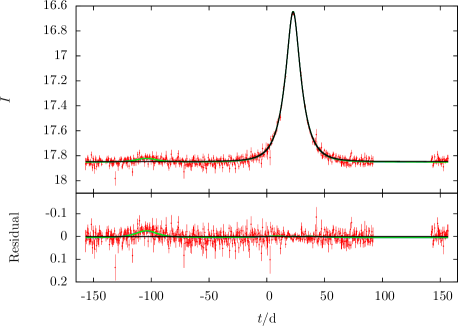
Figure 3: An example lightcurve from the simulations that required coverage to be extended to cover a feature far from the lightcurve peak. The upper panel shows the lightcurve ($I$-band magnitude) and the lower panel shows the Paczyński residual ($I$-band residuals from the single lens fit). Red points show the simulated data points with error bars, and black, green and blue lines are the best-fitting Paczyński model, the best-fitting static binary model and the true orbital motion model (largely hidden below the green static model curve) respectively. Only one data point in 24 is shown for clarity. The lightcurve shown is for that of an event by a stellar binary lens with $q=0.22$, $d\approx 8.6$ and $t_{\mathrm{E}}=14.9\text{~{}d}$. Usually, only data points that cover the inner $5t_{\mathrm{E}}$ are used, apart from some data points used to constrain the baseline magnitude (cf. the lightcurve for times $t>0\text{~{}d}$), however additional data points are used to fully cover the additional lightcurve feature down to baseline (cf. the lightcurve for $t<0\text{~{}d}$). Further details for the event can be found in Tables 4 and 5 in the online supplementary material.

To ensure that all the features of a lightcurve are covered, and that there is a good balance between the baseline, peak and features of the lightcurve when fitting (see the next section), the lightcurve is monitored continuously over the times $-5t_{\mathrm{E}}\leq t-t_{\mathrm{0}}<5t_{\mathrm{E}}$, and over $10.5t_{\mathrm{E}}\leq|t-t_{\mathrm{0}}|<9.5t_{\mathrm{E}}$ to sample the baseline. To ensure that all features are covered, if the magnification of the source rises above $A\geq A_{\mathrm{thresh}}=1.0062$, the coverage is extended so as to be continuous within one Einstein time-scale of the feature and continuous between the feature and $t=t_{\mathrm{0}}$. Figure 3 shows an example of a lightcurve where coverage had to be extended.

4 Measuring orbital motion

Ultimately we are interested in finding the fraction of binary microlensing events which show signs of orbital motion. To do this we must classify the events we simulate into those binary events that do show orbital motion, those that do not, and events that do not show binary signatures. To do this we fit each event first with a single lens model, and then those events which are poorly fit with this model, we fit with a static binary lens model. To evaluate the effectiveness of each stage of the fitting process, in addition to the fitting of the lightcurves simulated with orbiting binary lenses, we must also fit lightcurves simulated with point-mass lenses and static binary lenses.

4.1 Lightcurve modelling

The single lens model has five parameters: the time of closest approach $t_{\mathrm{0}}^{\mathrm{P}}$, the event time-scale $t_{\mathrm{E}}^{\mathrm{P}}$, the impact parameter $u_{\mathrm{0}}^{\mathrm{P}}$, the baseline magnitude $I_{\mathrm{b}}^{\mathrm{P}}$ and the blending fraction $f_{s}^{\mathrm{P}}$. We performed a $\chi^{2}$ minimization using the minuit routine from cernlib (James & Roos, 1975), with all parameters free; all parameters were unconstrained, except for $f_{s}^{\mathrm{P}}$, which was constrained to be within $0.0<f_{s}^{\mathrm{P}}<1.2$. For each event, seven single lens fits were performed, with different initial blending fractions, $f_{s}^{\mathrm{P}}=0.05$, $0.2$, $0.4$, $0.6$, $0.8$, $1.0$ and $1.2$. For each fit, the initial guesses for each parameter were: $t_{\mathrm{0}}^{\mathrm{P}}=0$, the time-scale was the true time-scale, the baseline magnitude was taken to be the magnitude of the first data point on the lightcurve, and the impact parameter was chosen such that at $t=t_{\mathrm{0}}^{\mathrm{P}}$ the magnitude of the event would be that of the brightest data point. This prescription works well for events which are well modelled by a single lens model, but not so for events with strong binary features, or events which are heavily blended and barely rise above baseline. It is therefore useful to eliminate events falling into the later category before performing the fitting, such that the only events that the single-lens model fails to fit are ones that show genuine signs of lens binarity. This cut will be described in the next subsection.

To fit the binary lens lightcurves, we found it necessary to split the events into caustic-crossing events and non-caustic-crossing events, and to fit each category using a different parametrization. The non-caustic crossing events we fitted with a standard parametrization, with a reference frame centred on the primary lens. The parameters are: the time of closest approach to the lens primary $t_{\mathrm{0}}^{\mathrm{S}}$, the event time-scale $t_{\mathrm{E}}^{\mathrm{S}}$, the impact parameter between the lens primary and the source $u_{\mathrm{0}}^{\mathrm{S}}$, the angle of the source trajectory to the binary axis $\theta_{\mathrm{0}}^{\mathrm{S}}$, the logarithm of the projected binary separation $\log d^{\mathrm{S}}$, the logarithm of the normalized secondary mass $\log m_{\mathrm{2}}^{\mathrm{S}}$, the baseline magnitude $I_{\mathrm{b}}^{\mathrm{S}}$ and the blending fraction $f_{s}^{\mathrm{S}}$. For brevity we introduce the vector notation

$$\vec{\mathfrak{p}}^{\mathrm{S}}=\left(t_{\mathrm{0}}^{\mathrm{S}},t_{\mathrm{E}}^{\mathrm{S}},u_{\mathrm{0}}^{\mathrm{S}},\theta_{\mathrm{0}}^{\mathrm{S}},\log d^{\mathrm{S}},\log m_{\mathrm{2}}^{\mathrm{S}},I_{\mathrm{b}}^{\mathrm{S}},f_{s}^{\mathrm{S}}\right),$$ (16)

to represent the parameter set of the standard binary parametrization.

For the number of lightcurves necessary to obtain a good statistical sample, a full search of the full binary lens parameter space is not computationally feasible, so we perform just one minimization per lightcurve. We must therefore pay special attention to the choice of initial guesses we use, firstly so as to maximize the chance of finding a good minimum, and secondly so as to treat the fitting of the static binary events comparably to the orbiting binary events. The static binary simulations are drawn from the same distributions as the orbiting binary simulations, the only difference being that the lens is frozen in the state it would be in at $t=t_{\mathrm{0}}$.

As we have simulated the microlensing events, we already have a perfect knowledge of the systems, and we can use this knowledge to obtain a good set of initial guesses. We note that at a given time, the state of an orbiting binary lens can be described by a static binary model. We can therefore describe our lens at time $t$ using the time dependent parameter set

$$\vec{\mathfrak{p}}(t)=\left(t_{\mathrm{0}},t_{\mathrm{E}},u_{\mathrm{0}},\theta_{\mathrm{0}}(t),d(t),q,I_{\mathrm{b}},f_{s}\right),$$ (17)

where we have used the same definitions and centre of mass reference frame as in the previous section. Note that only two of the parameters are time dependent, and so we can use the true values of the constant parameters as initial guesses, having applied the appropriate coordinate transformations. However, we are still left with the problem of choosing the guesses of $\theta_{\mathrm{0}}^{\mathrm{S}}$ and $d^{\mathrm{S}}$. We could choose $\theta_{\mathrm{0}}(t_{\mathrm{0}})$ and $d(t_{\mathrm{0}})$, but this would bias the fitting success probability unfairly towards static binary events: the initial guess would be the actual model used to simulate the data. Instead, we choose to use $d(t_{\mathrm{f}})$ and $\theta_{\mathrm{0}}(t_{\mathrm{f}})$, where $t_{\mathrm{f}}$ is the time of a feature in the lightcurve. We define a feature simply as any maximum in the lightcurve, or a maximum or minimum in the Paczyński residual (the residual of the true lightcurve with respect to the best fitting single lens model) with $|I-I_{\mathrm{Pac}}|>0.1$, where $I$ is the $I$-band magnitude of the true model, and $I_{\mathrm{Pac}}$ the $I$-band magnitude of the best fitting Paczyński model. As there are in general more than one feature, we choose the feature that gives the best $\chi^{2}(\vec{\mathfrak{p}}(t_{\mathrm{f}}))$. If the initial guesses for fits to static binary lightcurves are chosen in the same way, as if the binary were orbiting, then the initial guesses for static lenses should be worse than for orbiting lenses, as at the time of the chosen feature, the true orbiting lens magnification will exactly match the magnification of the initial guess static model. In reality, for $t_{\mathrm{f}}\approx t_{\mathrm{0}}$ there will likely be a bias in favour of static lenses and $t_{\mathrm{f}}\not\approx t_{\mathrm{0}}$ there will be a bias in favour orbiting lenses, but we do not believe this will affect results significantly. To fit the events, we again use the minuit minimizer, allowing all parameters to vary. All parameters are unconstrained, except for $f_{s}^{\mathrm{S}}$, which is constrained to the range $0<f_{s}^{\mathrm{S}}<1.2$.

While this method was suitable for events which showed smooth binary features, it is not always suitable for those events which exhibit caustic crossings. For these events, in addition to fitting with the standard parametrization, we also used the alternative parametrization of Cassan (2008). This replaces the parameters specifying the source trajectory $(t_{\mathrm{0}}^{\mathrm{S}},t_{\mathrm{E}}^{\mathrm{S}},u_{\mathrm{0}}^{\mathrm{S}},\theta_{\mathrm{0}}^{\mathrm{S}})$, with parameters that better reflect the sharp caustic crossing features of the lightcurve $(t_{\mathrm{en}}^{\mathrm{C}},t_{\mathrm{ex}}^{\mathrm{C}},s_{\mathrm{en}}^{\mathrm{C}},s_{\mathrm{ex}}^{\mathrm{C}})$ the times of a caustic entry and exit and the positions of the entry and exit on the caustic respectively, where $s_{\mathrm{en}}^{\mathrm{C}}$ and $s_{\mathrm{ex}}^{\mathrm{C}}$, are defined to be the chord length along the caustic, normalized such that $0\leq s_{\mathrm{en}}^{\mathrm{C}},s_{\mathrm{ex}}^{\mathrm{C}}<2$. Full details of the parametrization can be found in the Cassan (2008) paper. The parameter set we use for caustic-crossing events is therefore

$$\vec{\mathfrak{p}}^{\mathrm{C}}=\left(t_{\mathrm{en}}^{\mathrm{C}},t_{\mathrm{ex}}^{\mathrm{C}},s_{\mathrm{en}}^{\mathrm{C}},s_{\mathrm{ex}}^{\mathrm{C}},\log d^{\mathrm{C}},\log q^{\mathrm{C}},I_{\mathrm{b}}^{\mathrm{C}},f_{s}^{\mathrm{C}}\right),$$ (18)

where the parameter $\log m_{\mathrm{2}}^{\mathrm{S}}$ has been replaced by $\log q^{\mathrm{C}}$ as a matter of preference; the two parameters are related by $m_{\mathrm{2}}^{\mathrm{S}}=q^{\mathrm{C}}/(1+q^{\mathrm{C}})$.

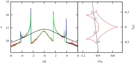
Figure 4: Example lightcurve and caustic map of an event where a non-adjacent caustic entry-exit pair was chosen for fitting with the Cassan (2008) parametrization. The lightcurve is shown in the left panel, where red points show the simulated data, the blue line is the true model and the green line is the static binary model. The right panel shows a map of the caustic of the static binary model, plotted in red, and the source trajectory, plotted in black. The numbers indicate the order of the caustic crossings. The static model has been adjusted by hand to aid clarity. Further details for the event can be found in Tables 4 and 5 in the online supplementary material.

The accurate calculation of the $s_{\mathrm{en}}^{\mathrm{C}}$ and $s_{\mathrm{ex}}^{\mathrm{C}}$ parameters is quite computationally expensive, compared to the calculation of a lightcurve, and needs to be repeated each time $d$ or $q$ changes. Also, despite the improved parametrization, the $\chi^{2}$ surface is still very complicated, especially in the $s_{\mathrm{en}}^{\mathrm{C}}$-$s_{\mathrm{ex}}^{\mathrm{C}}$ plane, containing many local minima. For these reasons we pursue a three stage minimization process. We begin by conducting a grid search over the entire $s_{\mathrm{en}}^{\mathrm{C}}$-$s_{\mathrm{ex}}^{\mathrm{C}}$ plane, with $128\times 128$ points spaced evenly in $s_{\mathrm{en}}^{\mathrm{C}},s_{\mathrm{ex}}^{\mathrm{C}}$, and with all other parameters, including the caustic crossing times, fixed at their true values, except for $\log d^{\mathrm{C}}$. $\log d^{\mathrm{C}}$ is fixed at a random value is chosen in from the range $\Delta\log d^{\mathrm{C}}=1.5(\log d(t_{\mathrm{ex}})-\log d(t_{\mathrm{en}}))$ or $\Delta\log d^{\mathrm{C}}=0.015$, whichever is greater, centred on the midpoint of $\log d$ between the caustic crossings, and where $d(t_{\mathrm{en}})$ and $d(t_{\mathrm{ex}})$ are the projected separations at the caustic entry and exit times respectively. The range of $\Delta\log d^{\mathrm{C}}$ is truncated, if necessary, to ensure that it only covers the caustic topologies at the time of the crossings. For the static lenses, $\log d^{\mathrm{C}}$ is chosen from a uniform distribution with the same range as if the lens were orbiting. The grid search is then refined by performing a second $128\times 128$ grid search over a box of side length $1/32$ about the grid point with the lowest $\chi^{2}$. Six $2\times 128\times 128$ grid searches are performed with different random values of $\log d^{\mathrm{C}}$. In cases where there are multiple caustic crossings, different pairs of caustic crossings are used to define $(t_{\mathrm{en}}^{\mathrm{C}},t_{\mathrm{ex}}^{\mathrm{C}},s_{\mathrm{en}}^{\mathrm{C}},s_{\mathrm{ex}}^{\mathrm{C}})$ for each grid search. Figure 4 shows an example lightcurve where the first caustic exit defines $(t_{\mathrm{en}}^{\mathrm{C}},s_{\mathrm{en}}^{\mathrm{C}})$ and the second caustic entry defines $(t_{\mathrm{ex}}^{\mathrm{C}},s_{\mathrm{ex}}^{\mathrm{C}})$.

The second stage of the fitting simply polishes the result of the grid search by performing a minimization over $s_{\mathrm{en}}^{\mathrm{C}}$ and $s_{\mathrm{ex}}^{\mathrm{C}}$, with all other parameters fixed, using minuit. In the final stage of the fitting, all parameters, except for $t_{\mathrm{en}}^{\mathrm{C}}$ and $t_{\mathrm{ex}}^{\mathrm{C}}$ are allowed to vary in a further minuit minimization. Again, all parameters were unconstrained, except for $f_{s}^{\mathrm{C}}$ which was constrained to the range $0<f_{s}^{\mathrm{C}}<1.2$. We found that, at all stages of the minimization for caustic crossing events, the minimization performed better when the first and last data points inside the caustic crossing were not considered in the fit. This is because, with the high cadence observations that we simulate, the point source is typically very close to the inside of the fold caustic, and hence is magnified by many orders of magnitude. This leads to unrealistic photometry in two ways: firstly, in a real detector, saturation would become a problem, and secondly, a real, finite, source would not be magnified in such an extreme way.

4.2 Classification of events

With the modelling procedures in place, we now describe the classification of the events. The classification is performed by a series of cuts based on the $\chi^{2}$ results of the fitting described in the last subsection. The first cut, the variability cut, removes events which do not show significant variability from the analysis. This is done, without fitting, by comparing the $\chi^{2}$ values of the simulated data relative to the true model, $\chi_{\mathrm{OM}}^{2}$, and relative to a constant lightcurve with no variability at the true baseline magnitude, $\chi_{\mathrm{b}}^{2}$. We exclude events that do not satisfy

$$\frac{\Delta\chi_{\mathrm{b}}^{2}}{n_{\mathrm{obs}}}\equiv\frac{\chi_{\mathrm{b}}^{2}-\chi_{\mathrm{OM}}^{2}}{n_{\mathrm{obs}}}>0.3,$$ (19)

where $n_{\mathrm{obs}}$ is the number of observations.

The second cut is used to classify events into single lens-like events, and binary lens-like events, or events that do not and do exhibit binary lens features in their lightcurves. Using the results of the single lens modelling, $\chi_{\mathrm{Pac}}^{2}$, the $\chi^{2}$ of the simulated data with respect to the single lens model, we define events that satisfy

$$\Delta\chi_{\mathrm{Pac}}^{2}\equiv\chi_{\mathrm{Pac}}^{2}-\chi_{\mathrm{OM}}^{2}>200$$ (20)

to be binary events, and those that do not to be single events. Binary events can then be split into caustic crossing binary events and smoothly varying events, or caustic crossing and smooth events respectively. We define a caustic crossing event as one where at least one data point is measured when the source is inside a caustic.

The final cut is based on the result of lightcurve fitting with binary models. Events that satisfy

$$\Delta\chi_{\mathrm{S}}^{2}\equiv\chi_{\mathrm{S}}^{2}-\chi_{\mathrm{OM}}^{2}>200$$ (21)

are classified as events that exhibit orbital motion (orbital motion events) and those that do not are classified as static events, where $\chi_{\mathrm{S}}^{2}$ is taken to be the $\chi^{2}$ of the best fitting static binary model. For smooth events this is the $\chi^{2}$ of the best fitting standard binary model, and for caustic crossing events it is the $\chi^{2}$ of the better fitting of the Cassan (2008) caustic crossing model or the standard binary model. In the case of the caustic crossing fits, the data points removed from the lightcurve do not contribute to $\chi_{\mathrm{OM}}^{2}$.

With these classifications in place, we can now define the binary detection efficiency and the orbital motion detection efficiency. The binary detection efficiency is the fraction of detectable microlensing events that show binary signatures

$$\epsilon_{\mathrm{BS}}\equiv\frac{N_{\mathrm{BS}}}{N_{\mathrm{ml}}},$$ (22)

where $N_{\mathrm{ml}}$ is the number of events satisfying $\Delta\chi_{\mathrm{b}}^{2}/n_{\mathrm{obs}}>0.3$, and $N_{\mathrm{BS}}$ is the number of events satisfying $\Delta\chi_{\mathrm{Pac}}^{2}>200$. The orbital motion detection efficiency is the fraction of binary events that show orbital motion signatures

$$\epsilon_{\mathrm{OM}}\equiv\frac{N_{\mathrm{OM}}}{N_{\mathrm{BS}}},$$ (23)

where $N_{\mathrm{OM}}$ is the number of events satisfying $\Delta\chi_{\mathrm{S}}^{2}>200$.

To be confident of our results we must quantify the effectiveness of the modelling prescriptions we use. We can do this by measuring the rate of false positives in our samples. To measure these rates we simulate both single lens events and static binary lens events, drawn from the same distributions as the orbiting lens events. These events then go through the same fitting procedure as the orbiting lens events and are subject to the same cuts. The binary lens false positive rate $\epsilon_{\mathrm{BS}}^{\rm single}$ is therefore the fraction of detectable single lens microlensing events that survive the $\Delta\chi_{\mathrm{Pac}}^{2}>200$ cut, and the orbital motion false positive rate $\epsilon_{\mathrm{OM}}^{\rm static}$ is the fraction of static binary lens events that survive the $\Delta\chi_{\mathrm{S}}^{2}>200$ cut.

5 Results

5.1 What fraction of events show orbital motion?

Table 1: Summary of the results for planetary lenses.

Orbit	static	circular
Single	48511	49226
Binary	1364	1366
Caustic	410	449
Caustic static	397	414
Caustic orbital motion	7	35
Smooth	954	917
Smooth static	931	883
Smooth orbital motion	23	34

Table 2: Summary of the results for stellar binary lenses.

Orbit	static	circular	eccentric
Single	4151	4046	4153
Binary	1413	1424	1385
Caustic	641	635	613
Caustic static	608	538	550
Caustic orbital motion	25	86	61
Smooth	772	789	772
Smooth static	764	743	729
Smooth orbital motion	8	46	43

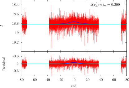
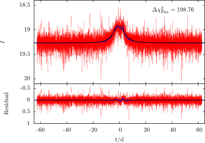
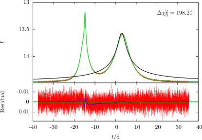
Figure 5: Example lightcurves of three events that narrowly failed one of the classification cuts. From top to bottom, the lightcurves failed the $\frac{\Delta\chi_{\mathrm{b}}^{2}}{n_{\mathrm{obs}}}\equiv\frac{\chi_{\mathrm{b}}^{2}-\chi_{\mathrm{OM}}^{2}}{n_{\mathrm{obs}}}>0.3$, $\Delta\chi_{\mathrm{Pac}}^{2}\equiv\chi_{\mathrm{Pac}}^{2}-\chi_{\mathrm{OM}}^{2}>200$, and $\Delta\chi_{\mathrm{S}}^{2}\equiv\chi_{\mathrm{S}}^{2}-\chi_{\mathrm{OM}}^{2}>200$ cuts, respectively. The upper panel of each subplot shows the lightcurve, and the lower panel the residual with respect to the appropriate model for the cut, i.e. the constant baseline ‘model’, the best fitting Paczyński model, and the best fitting static binary model in the top, middle and lower subplots, respectively. Colour coding is the same as in Figure 3, and the cyan line in the top subplot shows the constant baseline ‘model’. Further details for the events can be found in Tables 4 and 5 in the online supplementary material.

We begin by presenting and analyzing the results of the simulations as a whole, calculating the fraction of microlensing events in which we expect to see orbital motion events. Tables 1 and 2 summarize the results of the cuts described in the previous section, for planetary and stellar binary events respectively. It should be noted that in a small number of caustic crossing events, the fitting procedure failed, and so these events have been excluded from the analysis of the orbital motion detection efficiency, but not of the binary detection efficiency. These events are included in the Binary and Caustic rows of Tables 1 and 2, but not in the others. Figure 5 shows some lightcurves which were slightly below the threshold for each cut.

Table 3: Binary and orbital motion detection efficiencies.

Orbit		circular	eccentric
$q<0.01$	$\epsilon_{\mathrm{BS}}$	$0.0772\pm 0.0014$	–
$q<0.01$ Caustic	$\epsilon_{\mathrm{OM}}$	$0.061\pm 0.010$	–
$q<0.01$ Smooth	$\epsilon_{\mathrm{OM}}$	$0.0130\pm 0.0055$	–
$q<0.01$ All	$\epsilon_{\mathrm{OM}}$	$0.029\pm 0.005$	–
$q\geq 0.01$	$\epsilon_{\mathrm{BS}}$	$0.260\pm 0.004$	$0.251\pm 0.004$
$q\geq 0.01$ Caustic	$\epsilon_{\mathrm{OM}}$	$0.098\pm 0.011$	$0.060\pm 0.010$
$q\geq 0.01$ Smooth	$\epsilon_{\mathrm{OM}}$	$0.048\pm 0.006$	$0.045\pm 0.006$
$q\geq 0.01$ All	$\epsilon_{\mathrm{OM}}$	$0.070\pm 0.006$	$0.052\pm 0.006$

Table 3 shows the binary detection efficiency and orbital motion detection efficiency for both planetary and stellar binary lenses. It should be noted that the binary detection efficiency will be larger than for microlensing events with finite sources, as the effect of the finite source will be to smooth out sharper lightcurve features, and usually reduce the amplitude of deviations from the single lens model. This means that $\epsilon_{\mathrm{BS}}$ for planetary lenses is likely a significant overestimate, however, for stellar binary lenses the result is likely to be more realistic as binary lightcurve features tend to be stronger and have longer durations. The detection efficiencies presented have been corrected for systematic false positives from each fitting stage by subtracting the measured false positive rates $\epsilon_{\mathrm{BS}}^{\rm single}$ and $\epsilon_{\mathrm{OM}}^{\rm static}$ from the detection efficiencies measured for orbiting lenses. From a simulation of $10^{4}$ single lenses with no false positives we measured $\epsilon_{\mathrm{BS}}^{\rm single}=0_{-0}^{+4.7\times 10^{-5}}$, where the error quoted is a statistical $1\sigma$ confidence limit calculated using Wilson’s score method (Wilson, 1927; Newcombe, 1998b). To calculate the errors on the corrected detection efficiencies shown in the table, and on those we present in the next subsection, we use Wilson’s score method adapted for the difference of two proportions (Newcombe, 1998a, method 10). For planetary events we measured false positive rates of $\epsilon_{\mathrm{OM}}^{\rm static}=0.0241_{-0.0032}^{+0.0036}$ for smooth events and $\epsilon_{\mathrm{OM}}^{\rm static}=0.0173_{-0.0039}^{+0.0050}$ for caustic crossing events. For stellar binary events we measured $\epsilon_{\mathrm{OM}}^{\rm static}=0.0104_{-0.0022}^{+0.0028}$ for smooth events and $\epsilon_{\mathrm{OM}}^{\rm static}=0.0395_{-0.0050}^{+0.0056}$ for caustic crossing events. The overall orbital motion detection efficiencies were calculated as a weighted average of the detection efficiencies for smooth and caustic crossing events, once corrected for false positives.

While in many cases we may not be able to say that a lightcurve in our simulations definitively shows orbital motion signatures, due to relatively high rates of false positive detections, there is a clear excess of detections in the circular and eccentric orbit simulations relative to the static ones, though the detection of this excess is only marginal in smooth planetary events. Interestingly, there appears to be a discrepancy in the orbital motion detection efficiencies for stellar binary caustic crossing events. The same static orbit simulation results were used to calculate the corrected orbital motion efficiencies for both circular and eccentric orbits, which means that the measurements are not independent. Also, the eccentricity of the orbits allows the projected separation to take a wider range of values than the circular orbits, which means the false positive rate measured with the same distribution for circular orbits is likely an overestimate for eccentric orbits; for caustic crossing events the majority of false positives are caused by events with resonant caustic topology (see Figure 19 later in this section). We therefore believe the discrepancy to be caused largely due to a combination of a relatively large statistical fluctuation in the number of eccentric orbit events that do show orbital motion, and an overestimate of the false positive rate for eccentric orbits.

5.2 What affects the detectability of orbital motion?

We now investigate the effects that various system parameters have on the detectability of orbital motion. We look at the dependence of the orbital motion detectability on both the standard microlensing parameters and the physical orbital parameters, and compare them where appropriate. While we conducted two sets of simulations, one with circular orbits and one with eccentric orbits, we only present the results for those with circular orbits here, as both sets are in good agreement.

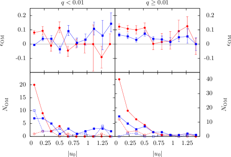
Figure 6: Plot of the orbital motion detection efficiency, corrected for systematic false positives (top panels), and the absolute number of orbital motion detections in the simulations (lower panels), against the impact parameter $|u_{\mathrm{0}}|$. Results are shown for lenses with planetary mass ratios (left) and binary star mass ratios (right). Red lines with filled squares show the results for caustic crossing events and blue lines with filled circles show the results for smooth events. In the upper panels a line marks zero orbital motion detection efficiency. All events had circular orbits, and in the lower panels results are shown for events where the lens components were in orbit (solid lines, filled points) and where they were held static for the calculation of the false positive rate (dashed lines, open points). Events have been binned into bins of equal width, and points plotted at the centre of the bin. Note that in the lower panels the scales are different.

We begin by looking at the dependence on the impact parameter, the sole parameter that determines the maximum magnification of a single lens microlensing event $A_{\mathrm{max}}=(u_{\mathrm{0}}^{2}+2)/(u_{\mathrm{0}}\sqrt{u_{\mathrm{0}}^{2}+4})$ (Paczyński, 1986). For all binary lenses, except wide stellar binaries, the central caustic is located near to the centre of mass, and so $u_{\mathrm{0}}$ determines whether or not the source will encounter this caustic. Figure 6 plots the orbital motion detection efficiency as a fraction of caustic crossing or smooth binary events (top panels), and the total number of orbital motion detections (bottom panels), against the impact parameter for both planets (left panels) and binary stars (right panels). In the plots, red lines represent data for caustic crossing events and blue lines for smooth events. In the top panel the orbital motion detection efficiency has been corrected for systematic false detections as described in the previous subsection, whereas the bottom panel shows the number of detections for both orbiting (solid lines, filled points) and static lenses (dashed lines, open points). Note that the orbital motion detection efficiency can be negative, due to statistical fluctuations, but if it is, the measurement should be consistent with zero. The events have been binned into bins of constant width, on the scale that they are plotted. It should also be noted, that the number of planetary events simulated was a factor of 9 larger than the number of stellar binary events.

The plots of orbital motion detection efficiency (from here on detection efficiency) against $|u_{\mathrm{0}}|$ for caustic crossing events show much the same trends for both planetary and stellar binary lenses, with significant detection efficiencies for high-magnification (low $|u_{\mathrm{0}}|$) events only, with no caustic crossing planetary detections for $|u_{\mathrm{0}}|\gtrsim 0.6$, and only a few for stellar binaries. This is due to the location of central and resonant caustics close to the center of mass, which the source can only cross in events with small $|u_{\mathrm{0}}|$. Consequently, for the events with larger $u_{\mathrm{0}}$, the source can only cross weaker secondary caustics, which in the case of wide binaries will typically move slowly, and in the case of close binaries are typically very small and are rarely crossed. The secondary caustics of close stellar binaries are significantly larger and stronger than those of planetary lenses, and so the chances of the source crossing them is higher, and the caustic has a longer time in which to change due to orbital motion as the source crosses it, leading to the small positive efficiency for $|u_{\mathrm{0}}|\gtrsim 0.6$. For smooth events, the planetary and stellar binary lenses show weak but opposing trends, with the efficiency increasing slightly as $|u_{\mathrm{0}}|$ increases for planetary events and decreasing slightly as $|u_{\mathrm{0}}|$ increases for stellar binary events, indicating that the impact parameter only plays a small role in orbital motion detectability for smooth lightcurves. Note however, that for both smooth and caustic crossing events the number of orbital motion detections, as opposed to the detection efficiency, is a strong function of $|u_{\mathrm{0}}|$, peaking at small values, due to the dependence of the binary detection efficiency on the impact parameter.

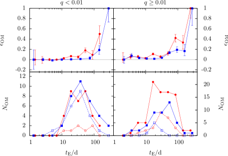
Figure 7: As Figure 6, but plotted against the event time-scale $t_{\mathrm{E}}$.

Figure 7 plots the detection efficiency against the event time-scale $t_{\mathrm{E}}$. All classes of binary event (planetary or binary, smooth or caustic crossing) show a strong detection efficiency dependence on the event time-scale. The reason for this dependence is simply because a longer time-scale allows the lens to complete a larger fraction of its orbit, and hence cause a larger change in the magnification pattern, during the time in which the source probes regions of the magnification pattern that deviate from that of a single lens. In the case of planetary lenses, it seems that a time-scale of greater than $\sim 10$ days is necessary for caustic crossing events and slightly longer for smooth events. Caustic crossing events show larger detection efficiency than smooth events, even at shorter time-scales. This is likely due to the high accuracy with which caustic crossing times, and the lightcurve shape around caustic crossings can be measured. In the case of OGLE-2006-BLG-109 this has allowed the orbital motion of the lens to be measured from data covering just $\sim 0.2$ percent of the orbit (Gaudi et al., 2008; Bennett et al., 2010). Smooth events in contrast require a much larger fraction of the orbit to cause significantly detectable changes in the lightcurve, and hence require a longer time-scale to achieve the same detection efficiency. However, typically it is possible for smooth features to cover a much larger fraction of the lightcurve than caustic crossing features, lessening the effect of this discrepancy.

For stellar binary lenses, orbital motion features can be can be detected effectively over almost the entire range of time-scales that we simulated, though with a low efficiency for time-scales below $\sim 40$ days for smooth events and $\sim 10$ days for caustic crossing events. For events with time-scales over $\sim 100$ days, the detection efficiency reaches $\sim 20$ percent for smooth events and $\sim 40$ percent for caustic crossing events. The detection efficiencies are similar for planetary events. The majority of planetary and binary events showing orbital motion have time-scales of around $\sim 10$–$40$ days, with few events at larger $t_{\mathrm{E}}$ due to the steep $t_{\mathrm{E}}^{-3}$ distribution at large time-scales (Mao & Paczyński, 1996). However, the strong dependence of $\epsilon_{\mathrm{OM}}$ on time-scale means that the slope of the high $t_{\mathrm{E}}$ tail of the distribution of orbital motion events is much shallower than $t_{\mathrm{E}}^{-3}$.

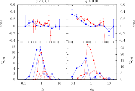
Figure 8: As Figure 6, but plotted against $d_{\mathrm{0}}$ the lens separation at time $t_{\mathrm{0}}$.

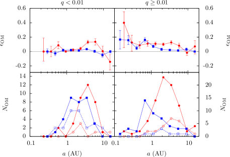
Figure 9: As Figure 6, but plotted against the semimajor axis $a$.

The plots of detection efficiency against projected separation $d_{\mathrm{0}}$ (Figure 8) and semimajor axis $a$ (Figure 9) tell largely the same story. The detection efficiency in stellar binaries has a significant inverse dependence on both $d_{\mathrm{0}}$ and $a$, as would be expected from the dependence of orbital velocity of semimajor axis. However, the behaviour for planetary lenses is less intuitive: for caustic crossing events, there is a significant peak in the detection efficiency at $a\sim 4$ AU, and a peak/shoulder at $d_{\mathrm{0}}\sim 2$. There is a second peak in $\epsilon_{\mathrm{OM}}$ with $d_{\mathrm{0}}$. The two peaks occur at values of $d_{\mathrm{0}}$ where the boundaries between caustic topologies occur for the highest mass ratio planets. It is at these boundaries that, for a small change in projected separation $\mathrm{d}(\log d)$, the largest changes in the caustics occur. The peak in $\epsilon_{\mathrm{OM}}$ against $a$ at $a\sim 4$ AU for caustic crossing planetary events is accompanied by a hint of a peak at small values of $a$. The peak at $a\sim 4$ AU can be explained by considering the typical scale of the Einstein ring, and by considering the trend of $\epsilon_{\mathrm{OM}}$ with the event time-scale. The typical size of the Einstein ring for a microlensing event is $2$-$3$ AU, but as seen in Figure 7, orbital motion effects typically occur in events with larger time-scales. As the time-scale is correlated with the Einstein ring size, and caustic crossing events typically occur in systems with $d_{\mathrm{0}}\sim 1$, the peak orbital motion detection efficiency occurs at a semimajor axis slightly above the typical Einstein ring size, at $a\sim 4$ AU. The increase in orbital velocity as $a$ decreases likely causes the second weaker peak in $\epsilon_{\mathrm{OM}}$ at smaller $a$. Little can be said about the trend of $\epsilon_{\mathrm{OM}}$ with $a$ for smooth planetary events as small numbers of events, and the distribution of Einstein radius sizes serves to smear out any obvious trends. However, when plotted against $d_{\mathrm{0}}$, $\epsilon_{\mathrm{OM}}$ does increase towards smaller values of $d_{\mathrm{0}}$, as would be expected from orbital velocity considerations.

Returning to the caustic crossing stellar binary events, $\epsilon_{\mathrm{OM}}$ flattens off as $a$ increases to $\sim 4$ AU, before dropping to zero. This flattening likely has the same cause as the peak for planetary caustic crossing events. We see the more intuitive inverse trend in stellar binaries because of the stronger and larger magnification pattern features that they exhibit, and the larger range of $d$ over which the caustics have a significant size. This results in a distribution of events over $a$ and $d_{\mathrm{0}}$ which is broader and somewhat less peaked than for planetary events (see the lower panels of Figures 8 and 9). This allows the inverse relationship between orbital velocity and semimajor axis to have a greater influence on the trend in the orbital motion detection efficiency. We note that the reason we see such a complicated relationship between $\epsilon_{\mathrm{OM}}$ and $a$ and $d_{\mathrm{0}}$, but not for example between $\epsilon_{\mathrm{OM}}$ and $t_{\mathrm{E}}$, is that the orbital separation affects the orbital velocity in a relatively simple way and caustic size and strength in a complicated way, whereas $t_{\mathrm{E}}$ only affects, or more accurately is the result of, a fairly simple dependence on a single factor in the detection of orbital motion, the source speed.

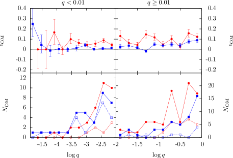
Figure 10: As Figure 6, but plotted against the mass ratio $q$.

Figure 10 plots the detection efficiency against the mass ratio $q$. Treating both planetary and stellar binary lenses together, there is a trend of increasing detection efficiency with increasing $q$, for both smooth and caustic crossing events. However, for caustic crossing events, this increase is very shallow, with a factor of $\lesssim 3$ increase over three decades in $q$, from $\log q\approx-3$ to $\log q=0$. For smooth events, there is a stronger trend, with the detection efficiency being effectively zero for $\log q\lesssim-3.5$, while rising from $\sim 1$ percent to $\sim 10$ percent over the range $-3.5\lesssim\log q<0$. These shallow dependencies are somewhat unexpected in relation to the somewhat stronger $q^{0.5}$ dependence of the binary detection efficiency, which derives directly from the dependence of caustic size on $q$ (Han, 2006). However, the orbital detection efficiency effectively divides through by this dependence (unlike the curves of the number of orbital motion detections, which show a strong dependence on $q$), to leave a very shallow orbital motion detection efficiency curves. The other effect that $q$ has on the lightcurve features is to make them stronger as $q$ increases. In caustic crossing events the caustic features are usually strong, independent of the value of $q$, and hence the caustic crossing events curve is shallower than the curve for smooth events, for which the dependence of the feature strength on $q$ is much more important.

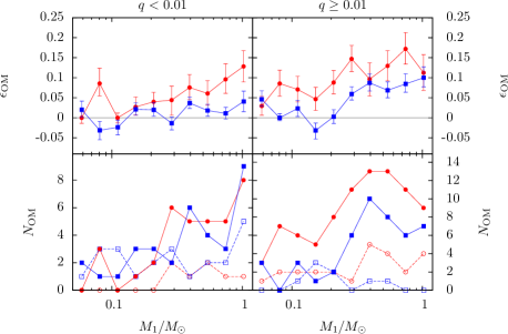
Figure 11: As Figure 6, but plotted against the primary lens mass $M_{\mathrm{1}}$.

Figure 11 shows the detection efficiency plotted against the primary lens mass. The dependence is as expected for both mass ratio regimes and for both types of binary event, increasing as the mass of the primary increases. The trend is strongest in smooth, stellar binary events.

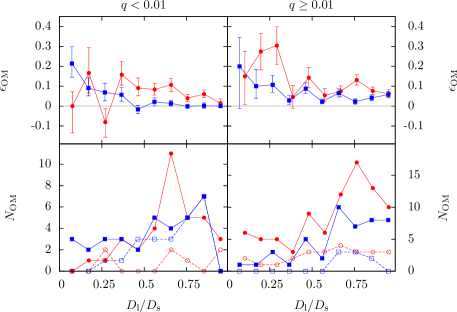
Figure 12: As Figure 6, but plotted against the lens distance $D_{\mathrm{l}}$.

Figure 12 plots the detection efficiency against the lens distance. In all cases, a trend of increasing detection efficiency with decreasing lens distance is seen, though caustic crossing events suffer from small number statistics at low values of $D_{\mathrm{l}}/D_{\mathrm{s}}$. Note however, that the frequency distribution (plotted in the lower panels of Figure 12) of orbital motion events, once false positives have been approximately accounted for, is different, being peaked at $D_{\mathrm{l}}/D_{\mathrm{s}}\sim 0.7$.

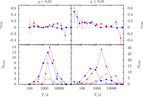
Figure 13: As Figure 6, but plotted against the orbital period $T$.

Figure 13 shows the detection efficiency plotted against the orbital period. Both types of stellar binary event show a significant inverse trend. Planetary caustic crossing events show a peak, and stellar caustic crossing events a flattening, at large periods. These features correspond directly to similar features in the curves of $\epsilon_{\mathrm{OM}}$ with $a$ and will have the same cause.

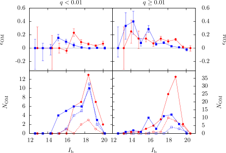
Figure 14: As Figure 6, but plotted against the baseline magnitude $I_{\mathrm{b}}$.

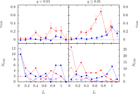
Figure 15: As Figure 6, but plotted against the fraction of baseline flux associated with the source $f_{s}$.

Figures 14 and 15 plot the detection efficiency against the baseline magnitude $I_{\mathrm{b}}$ and blending fraction $f_{s}$ respectively. For our purposes, the primary effect of both parameters is to affect the accuracy with which microlensing variations can be measured in the lightcurve. For a fixed observing setup, the baseline magnitude determines the photometric accuracy, which should lead to a trend of increasing detection efficiency with decreasing magnitude. This is seen to a certain extent in all cases, but brighter events may suffer significantly from blending, due to faint source stars falling entirely within the large point spread function of a much brighter star. Blending determines the relative strength of features in the lightcurve, and as such has a much more significant effect on the detection of smooth binary features, which have a continuous range of shapes and sizes, compared to the effect on caustic crossings which are typically sharp and very strong, at least when finite sources are not considered. It is no surprise, therefore, that smooth stellar binary events show a significant increase in orbital motion detection efficiency with blending fraction. This is less obvious in planetary lenses, likely because the smooth lightcurve features of planetary lenses are often very weak and difficult to detect even without the hindrance of the blending, and would not permit the measurement of higher order effects for any value of blending fraction. It is more surprising, perhaps, that caustic crossing events show a significant dependence on blending, as in the simulations all caustic crossing events were detected as binaries, regardless of blending. This implies that, at least in some orbital motion detections in caustic crossing events, the additional smooth features in the lightcurve, such as peaks and shoulders due to cusp approaches outside the caustic, and features due to fold caustic approaches within the caustic, play an important role in the detection of orbital motion (e.g. lightcurves a and e in Figure 21 in the next subsection).

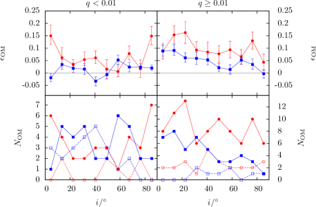
Figure 16: As Figure 6, but plotted against the orbital inclination $i$

Figure 16 plots the detection efficiency against inclination. There is little evidence for any significant dependence on inclination for all caustic crossing events, and for smooth planetary events. There is however a stronger trend for smooth stellar binary events, the detection efficiency decreasing as the inclination increases. This would be expected in systems where $a/r_{\mathrm{E}}\lesssim d_{\mathrm{c}}$, the boundary between close and resonant caustic topologies, where a reduction in the projected separation due to inclination would reduce the size of the caustics and reduce the detectability of both binary features and orbital motion signatures. Unfortunately, due to the similar effects of inclination and eccentricity on the projected orbit, the data from the eccentric orbit simulations did not show any dependence of $\epsilon_{\mathrm{OM}}$ with eccentricity. This however implies that the effects of eccentricity on the orbital motion detection efficiency are not likely to be significantly stronger than those of inclination.

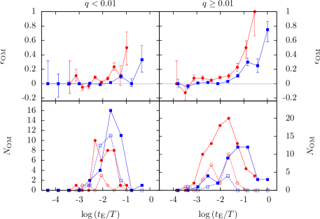
Figure 17: As Figure 6, but plotted against the ratio of microlensing to orbital time-scales $R_{\mathrm{T}}=t_{\mathrm{E}}/T$

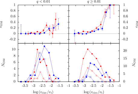
Figure 18: As Figure 6, but plotted against the ratio of orbital and source velocities $R_{\mathrm{v}}=v_{\mathrm{circ}}/v_{\mathrm{t}}$

It is important not just to consider the system parameters in isolation, but also their combined effects on the orbital motion detection efficiency. For example, Dominik (1998) introduced two dimensionless ratios to describe the magnitude of orbital motion effects on a binary lens:

$$R_{\mathrm{T}}=\frac{t_{\mathrm{E}}}{T},$$ (24)

the ratio of time-scales, and

$$R_{\mathrm{v}}=\frac{v_{\mathrm{circ}}}{v_{\mathrm{t}}},$$ (25)

the ratio of velocities, where $v_{\mathrm{circ}}=a/2\pi T$ is the circular velocity of the orbit. These ratios attempt to encapsulate the most important factors that determine if an event will show orbital motion features. Figures 17 and 18 plot the detection efficiency against $R_{\mathrm{T}}$ and $R_{\mathrm{v}}$ respectively. Both ratios prove to be good descriptors of the orbital motion detection efficiency, with $\epsilon_{\mathrm{OM}}$ showing strong increasing trends as $R_{\mathrm{T}}$ and $R_{\mathrm{v}}$ increase, across all mass ratios and lightcurve types, though with a lower significance in planetary events. It would even seem that, in the case of smooth events, there exists a threshold value of the ratios, below which the orbital motion detection efficiency is negligible. For the ratio of time-scales, the threshold is $\log R_{\mathrm{T}}\approx-2$ for both planetary and stellar binary lenses, while for the ratio of velocities the value appears to be more dependent on the mass ratio, taking values of $\log R_{\mathrm{v}}\approx-2.5$ for planetary lenses, and $\log R_{\mathrm{v}}\approx-2.75$ for stellar binary lenses. There may be similar thresholds for caustic crossing events, but at smaller values of $R_{\mathrm{T}}$ and $R_{\mathrm{v}}$.

5.3 Are there two classes of orbital motion event?

Gaudi (2009) has suggested that orbital motion can affect the lightcurves of microlensing events in two ways. In the first scenario, the orbital motion effects are dominated by rotation in the lens, as the orientation of binary axis changes during the time between two widely separated lightcurve features. The second type of effect is due to changes in the projected separation over the course of a single lightcurve feature such as a resonant caustic crossing. In this subsection we will describe the typical features of each type of event before investigating to what extent orbital motion events can be classified in such a way.

Gaudi (2009) describes the separational class of event as typically occurring in archetypal binary microlenses with resonant caustic crossings. If the binary’s orbit is inclined, the projected separation of the lenses changes, causing a stretching or compression of the resonant caustic. If the projected separation is close to a boundary between caustic topologies, $d\sim d_{\mathrm{c}}$, or $d\sim d_{\mathrm{w}}$, the changes in the caustic structure can be very rapid. If the microlensing event occurs while the changes are happening, and the source crosses, or passes close to, the caustics, there is a very good chance of detecting the orbital motion. As a whole though, the changes in caustic structure during the caustic crossing time-scale will be fairly small, e.g. the difference in caustic crossing time between the static lens and the orbiting lens may be of order minutes to hours (cf. the orbital period of several years). It is only the extremely good accuracy with which caustic crossings can be measured and timed that facilitates the high orbital motion detection probability. These changes to the caustic shape will often be more significant than the changes in orientation of the caustic due to rotation, and so we class them as separational orbital motion effects.

Gaudi (2009) described the rotational class of event as occurring when a source encounters two disjoint caustics of a typically close topology lens. In the time between the two caustic encounters, which are separated by a time $\Delta t\sim t_{\mathrm{E}}$, the lens components have time to rotate and show detectable signatures of orbital motion. We extend the class by considering the important effect to be the long baseline over which binary lensing features can be detected. If binary lens features are detectable across a significant fraction of the lightcurve then a significant amount of rotation can occur in the lens while the features are detectable. Up to now, our discussion has focused mainly on caustic features, whether the source crosses them or not, but, in stellar binary lenses especially, the magnification pattern of the lens can differ significantly, if subtly, from the single lens form over large parts of the pattern, and well away from caustics. For example, in close binary lenses, there is a region of excess magnification that can stretch the entire distance between the facing cusps of the central and secondary caustics. In stellar binary lenses, this can extend for distances larger than an Einstein radius. In planetary lenses the magnification excesses are weaker, but there tends to be a large region of demagnification between the two planetary caustics. If lenses with such features rotate rapidly, then the source may encounter them in such a way that a static lens interpretation of the lightcurve features is not possible, and lens rotation must be invoked.

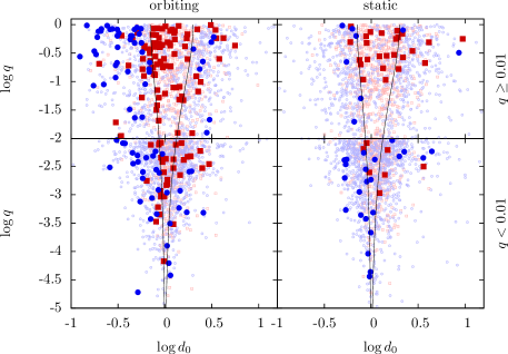
Figure 19: Scatter plot of $q$ against $d_{\mathrm{0}}$ for microlensing events with detectable binary signatures. Caustic crossing events are plotted with red squares, and smooth events with blue circles. Events classified as orbital motion events are plotted with larger, darker filled points, and those classified as static with smaller, lighter, open points. The black lines show the positions of the caustic topology boundaries.

We begin by looking for evidence of two classes of event in the locations of the orbital motion events in the $d_{\mathrm{0}}$-$q$ plane. Figure 19 plots $q$ against $d_{\mathrm{0}}$ for all binary events; events which do not show orbital motion signatures are plotted with small, open points with light colours, whereas those that do are plotted with large, filled points with darker colours. Caustic crossing events are plotted with red squares, and smooth events with blue circles. Upper panels show stellar binary lenses and lower panels show planetary lenses, while the left panels show orbiting lenses and the right panel show static lenses. The black lines show the boundaries between the caustic topologies (equations 7 and 8). It is immediately clear that caustic crossing and smooth orbital motion events reside in different regions of the $d_{\mathrm{0}}$-$q$ plane, with virtually all events within the intermediate topology regime being caustic crossing. Almost all smooth orbital motion events are located in the close topology region. This broadly reflects the underlying pattern for all binary events, and is not in itself evidence of two classes of orbital motion events, but is instead a result of different caustic sizes in the different caustic topologies.

Another feature of the plot is the clustering of caustic crossing orbital motion events near the boundary of the close and intermediate topologies. It is close to the topology boundaries that the changes in projected separation cause the largest changes in the caustics. It is however difficult to attribute this clustering to faster caustic motions due to separational changes, as orbital velocity is inversely correlated with $d_{\mathrm{0}}$, and so there should be more orbital motion events at smaller values of $d_{\mathrm{0}}$ in any case. In support of the existence of a separational class, there is a hint of clustering against the resonant-wide boundary. However, the caustic size peaks at both topology boundaries, as the single resonant caustic stretches before splitting apart into central and secondary caustics, possibly meaning that simply the increased size of the caustics causes the increased density of detections.

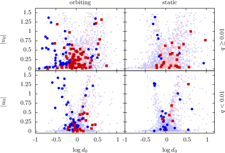
Figure 20: As Figure 19 but showing $|u_{\mathrm{0}}|$ plotted against $d_{\mathrm{0}}$.

Figure 20 plots the impact parameter against $d_{\mathrm{0}}$ and is very useful in separating different kinds of binary event, especially for planetary lenses. The events follow a distinctive pattern, with a large clump of events centred at $|u_{\mathrm{0}}|\sim 0$ and $\log d_{\mathrm{0}}\sim 0$ which consists of high-magnification events that encounter the central or resonant caustic. At very small $|u_{\mathrm{0}}|$ this clump extends over a significant range in $d_{\mathrm{0}}$, but narrows as $|u_{\mathrm{0}}|$ increases, to its narrowest point at $|u_{\mathrm{0}}|\sim 0.3$, corresponding to the maximum size of the region affected by resonant caustics (or at larger $|u_{\mathrm{0}}|$ for stellar binaries). As $|u_{\mathrm{0}}|$ increases, the plot shows a distinctive ‘V’ shape, with no binary signatures being detected for events with $d_{\mathrm{0}}\sim 0$. This ‘V’ shape arises as, in events with larger $|u_{\mathrm{0}}|$, the source passes through regions of the magnification pattern that can only contain secondary caustics, and does not enter the regions containing central or resonant caustics, i.e. the binary features in lenses with $d_{\mathrm{0}}\sim 1$ only occur in regions of the magnification pattern that the sources with large $|u_{\mathrm{0}}|$ do not probe.

The events which occur on the branch with large $|u_{\mathrm{0}}|$ and large $d_{\mathrm{0}}$ are caused by wide topology lenses, and therefore involve only a single secondary caustic encounter. The rotation of these lenses is typically very slow, and over the short duration of the binary features (typically of order a day), the lens completes only a very small fraction of its orbit. This points towards separational changes being the dominant effect in the detection of orbital motion features in events on this branch, even with the enhancement of rotational velocity due to the solid body ‘lever arm’.

The events that occur on the branch with large $|u_{\mathrm{0}}|$ and small $d_{\mathrm{0}}$ are largely smooth events, with the occasional caustic crossing event. The smooth events are likely caused by the source crossing the large cusp extensions that occur in close binary lenses, suggesting that they will belong to the rotational class of events.

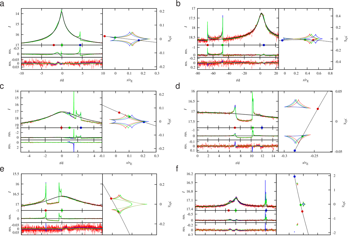
Figure 21: Example lightcurves of simulated events affected by separational type orbital motion effects. In each subfigure, the left panels show the lightcurve, its residual with respect to the best fitting Paczyński model and its residual with respect to the best fitting static binary model, from top to bottom respectively. Simulated data is shown in red, the Paczyński model in black, the static binary model in green and the true model in blue. The right panel shows the caustics at various times, and the source trajectory in the frame of reference rotating with the projected binary axis. The source trajectory is plotted in black, and the caustics are colour coded according to the time. Coloured points on the lightcurve panel show the time at which the caustic was in the state shown, and the coloured points on the source trajectory show the position of the source at this time. The parameters of the microlensing events can be found in Tables 4 and 5 in the online supplementary material.

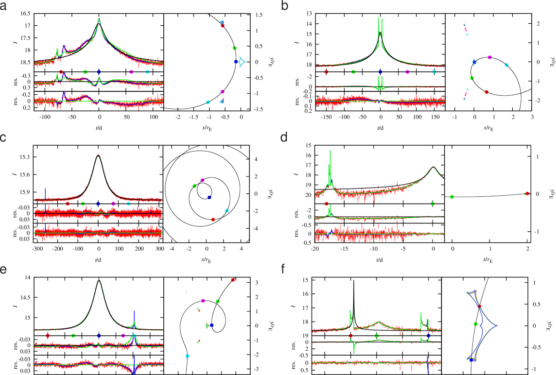
Figure 22: As Figure 21, but showing example lightcurves of simulated events affected by rotational type orbital motion effects.

Table 4: Microlensing parameters of example lightcurves in the paper.

Figure	Orbit†	$u_{\mathrm{0}}$	$\theta_{\mathrm{0}}/\degr$	$d_{\mathrm{0}}$	$q$	$t_{\mathrm{E}}/$d	$I_{\mathrm{b}}$	$f_{s}$
3	C	0.48	307	8.64	0.22	14.9	17.9	1.04
4	S	-0.091	186	0.95	0.054	14.7	19.2	0.59
5top	C	1.43	315	5.23	0.030	7.5	18.8	0.41
5middle	C	-0.16	155	0.61	0.14	12.6	19.3	0.082
5bottom	C	0.37	255	2.92	0.21	6.9	14.5	0.93
21a	C	-0.011	255	1.06	0.0016	26.2	17.1	0.19
21b	C	-0.024	285	1.31	0.0076	132.2	18.7	0.067
21c	C	-0.071	81	1.04	0.0015	12.2	19.6	0.71
21d	C	0.22	265	0.87	0.00045	65.7	18.0	0.38
21e	C	0.16	169	0.94	0.0038	26.3	17.3	0.15
21f	E	-0.20	16	0.55	0.49	14.8	17.3	0.073
22a	C	0.15	52	0.57	0.33	54.6	18.6	0.67
22b	C	0.033	69	0.45	0.56	88.3	18.2	0.72
22c	C	-0.56	353	0.18	0.30	49.3	16.0	1.04
22d	C	-0.076	245	2.38	0.0059	9.0	20.0	1.04
22e	E	-0.33	163	0.34	0.29	82.4	15.3	0.96
22f	E	0.21	77	0.79	0.29	24.3	18.7	0.20

†C–circular orbit, S–static orbit, E–eccentric orbit

Table 5: Physical parameters of example lightcurves in the paper.

Figure	Orbit	$M_{\mathrm{1}}/M_{\sun}$	$M_{\mathrm{2}}$	$a/$AU	$T/$d	$e$	$i/\degr$‡	$v_{\mathrm{t}}/$km s-1	$D_{\mathrm{l}}/$kpc
3	C	0.084	0.018 $M_{\sun}$	10.7	39799	0	214	134.8	5.75
4	S	0.70	0.038 $M_{\sun}$	1.88	1090	0	300	215.7	7.40
5top	C	0.058	0.0018 $M_{\sun}$	4.46	14047	0	173	196.3	6.04
5middle	C	0.13	0.017 $M_{\sun}$	1.22	1298	0	311	183.8	5.95
5bottom	C	0.10	0.021 $M_{\sun}$	3.52	6852	0	112	282.8	6.43
21a	C	0.55	0.89 $M_{\mathrm{Jupiter}}$	5.82	6924	0	93	167.3	6.12
21b	C	0.75	6.0 $M_{\mathrm{Jupiter}}$	4.32	3767	0	115	39.8	6.01
21c	C	0.27	0.43 $M_{\mathrm{Jupiter}}$	0.51	256	0	243	63.2	7.91
21d	C	0.89	0.42 $M_{\mathrm{Jupiter}}$	3.83	2899	0	136	88.8	2.13
21e	C	1.17	4.7 $M_{\mathrm{Jupiter}}$	3.42	2130	0	56	173.5	7.19
21f	E	0.21	0.10 $M_{\sun}$	0.61	306	0.92	102,216	183.0	6.90
22a	C	0.56	0.18 $M_{\sun}$	1.88	1098	0	16	101.2	2.44
22b	C	0.38	0.21 $M_{\sun}$	1.69	1044	0	40	57.4	2.69
22c	C	0.68	0.20 $M_{\sun}$	0.65	205	0	30	115.8	5.97
22d	C	0.65	4.0 $M_{\mathrm{Jupiter}}$	2.70	2005	0	2	218.3	7.75
22e	E	0.59	0.17 $M_{\sun}$	1.35	656	0.77	303,213	68.2	5.56
22f	E	0.39	0.11 $M_{\sun}$	2.14	1609	0.18	2,143	187.0	5.64

‡For events with eccentric orbits, two values of inclination are quoted, representing inclinations about two orthogonal axes on the sky. The effect of this second inclination is absorbed into the source trajectory for circular orbits, and to first order can be reduced to the range $0\degr\leq i\leq 90\degr$.

Unfortunately it is difficult to attribute the cause of any one grouping of orbital motion events in Figures 19 and 20 to either the rotational or the separational class, partly because both types of motion will affect each event to some extent. Despite this, it is possible to classify many individual events as either a separational or rotational event. Figures 21 and 22 show example lightcurves of both classes of orbital motion event, rotational and separational, respectively. The plots show the lightcurve in the upper left panels, with simulated data in red, the true model in blue, the best fitting static binary model in green and the best fitting single lens model in black. Also shown are the residuals from the single lens model and the static binary model in the middle and lower left panels respectively. Shown in the right panel is a plot of the source trajectory, shown in black, and snapshots of the caustics at various times during the event, shown in different colours. The coloured points on the time axis of the lightcurve show the time at which the caustic snapshots occurred, and the coloured points on the source trajectory show the position of the source at these times. The source trajectory and caustics are shown in the frame of reference that rotates with the binary axis, with its origin at the centre of mass. In this frame, rotation of the lens causes the source trajectory to appear curved, and changes in lens separation cause the caustics to change shape and move. Note that in event f in Figure 21, and events e and f in Figure 22, the lens orbits are eccentric, so that the source does not travel along the shown trajectory at a constant rate.

Figure 21 shows examples of separational events. In each example the source trajectory appears relatively straight, indicating that the lens rotates little; however, in each case the caustics move significantly. Events a, b, c and e all involve resonant caustic crossings, and conform well to the picture described by Gaudi (2009). Event d could be described as the encounter of two disjoint caustics, similar to the original description of the rotational class of events by Gaudi (2009), but other than the close topology, the event is remarkably similar to event e; the source trajectory is slightly curved, but it is clear that separational effects are dominant. At first glance, event f would clearly fit into the picture of disjoint caustic encounters, but the source trajectory reveals that rotation plays only a minor role. In this event, a static fit to just the features about $t=t_{\mathrm{0}}$ would suggest a close encounter with a large secondary caustic at $t\approx 1.5t_{\mathrm{E}}$, but instead changes in the binary’s separation cause the source to not just encounter, but cross a now much smaller secondary caustic at $t\approx 2t_{\mathrm{E}}$.

In contrast to Figure 21, the source trajectories in Figure 22 show significant curvature. Event a fits the description of rotational events by Gaudi (2009) exactly. The source first encounters a secondary caustic, but the rotation of the lens causes the source to pass the opposite side of the central caustic. Rotation also prevents the source from crossing the magnification excess between central caustic and the other secondary caustic. During the entire event, separational changes cause only slight changes in the caustics. In event c the rotation is more extreme, but the caustics smaller. The binary features are therefore more subtle, being caused by small magnification excesses between the caustics; the secondary caustics being located at $\sim(-3,\pm 4)$, and the central caustic at $\sim(0,0)$. The rotation of the lens causes the source to cross each excess more than once, and there are several minor deviations visible in the residual between the static and true model of the event. Event d, while being caused by a wide lens, expected to rotate slowly, is clearly caused by rotation. During the event, there are virtually no separational changes, but the precision with which the secondary caustic crossing and cusp approach features constrain the source trajectory mean that the very slight rotation which brings the source closer to the central caustic is detectable. Events b and e both show strong signs of rotation in their source trajectories, but separational changes are also important. While we assign them to the rotational class of event, in reality they may better fit into a third, hybrid class. Event f also shows signs of both rotational and separational orbital motion effects, but we assign it to the rotational class because without rotation the second caustic crossing would be significantly shorter.

6 Discussion

6.1 Limitations of the study

The questions that we wanted to answer in this work were: what fraction of microlensing events observed by the next generation surveys will be affected by orbital motion and what type of events are the effects likely to be seen in? While we do not claim to have fully answered these questions, we do feel that this work represents an important step in that direction. The simulation of the photometry is slightly optimistic, and does not include the effects of weather and the systematic differences in the site conditions and observing systems, distributed across the Globe, that would make up the network of telescopes needed for a continuous monitoring microlensing survey. The observing setup we simulated is in some respects more like a space based microlensing telescope than a ground based network. However, the photometric accuracy that we simulated is not too optimistic, and the differences between the static and orbiting simulations show that orbital motion plays a significant role in a significant fraction of microlensing events.

As discussed in Section 3, our choice of models will not fully answer the question of how many microlensing events with orbital motion effects will be seen, however, they do provide a good order of magnitude estimate. The binary detection efficiencies we find assume that all stars have a companion, and so must be adjusted accordingly to account for this. For example, current estimates suggest that only $\sim 33$ percent of stellar systems are binaries (e.g. Lada, 2006), so assuming that a next generation microlensing survey detects $\sim 2000$ events per year we can expect to see $\sim 30$ stellar binary microlensing events showing orbital motion signatures per year. However, the true rate may be higher as the mass ratio distribution that we use for stellar binaries is not realistic; the real distribution is likely to be peaked in the range $0.1\leq q\leq 1$ (e.g. Duquennoy & Mayor, 1991). A similar calculation for planetary lenses, assuming the fraction of stars hosting planets is $\sim 0.5$, yields a detection rate of $\sim 1.5$ caustic crossing orbital motion events per year. Again, this estimate is affected significantly by our assumptions. Our mass ratio distribution is optimistic, with current microlensing results suggesting an inverse relation between planet frequency and mass ratio in the regions microlensing is sensitive to (Sumi et al., 2010; Gould et al., 2010). This implies our estimate is optimistic, but we have also assumed there is only one planet per system. Many multiplanet systems have been discovered to date (e.g. Gaudi et al., 2008; Fischer et al., 2008), and they are thought to be common. The microlensing planet detection efficiency in multiplanet systems is increased, as the planets are spread over a range of semimajor axes. This will somewhat compensate for the overestimate due to the incorrect mass ratio distribution.

The major limitation of this work is that finite source effects are not considered. The finite size of the source acts to smooth out the extreme magnification peaks as a source crosses a caustic, limiting the precision with which magnifications can be measured, and caustic crossings timed, and thus plays an important role in orbital motion detection. However, in most cases, the caustic entry times can still be timed accurately if the caustic crossing is monitored with high enough cadence. In some cases the effect may increase the detectability of orbital motion as the source will probe more of the magnification pattern, especially when a source travels approximately parallel to and very close to the inside of a fold caustic, producing additional peaks between the caustic crossings. We cannot quantitatively estimate the effects that finite source size has on the orbital motion detection efficiency, but we do not believe it will significantly affect our order of magnitude estimates. Unfortunately including finite source sizes in the modelling of a microlensing event increases the required computation time by several orders of magnitude, so the effect could not easily be included in the simulations without significantly reducing the sample size.

6.2 Comparison with observations

While our simulations are more representative of future microlensing surveys, it is possible for us to compare the results of our simulations with the results of the current microlensing observations. Current microlensing planet searches using the survey/follow-up strategy routinely achieve a cadence similar or better than that expected for future high-cadence surveys for a small number of microlensing events per year (e.g. Dong et al., 2009). We can therefore compare the detection efficiency of orbital motion in the events where planets are detected. At the time of writing, there were 10 published detections of planets by microlensing (Bond et al., 2004; Udalski et al., 2005; Beaulieu et al., 2006; Gould et al., 2006; Gaudi et al., 2008; Bennett et al., 2008; Dong et al., 2009; Sumi et al., 2010; Janczak et al., 2010), and of these, 7 had high cadence coverage of a significant proportion of the lightcurve. In two of these events the orbital motion of the planet was detected (Gaudi et al., 2008; Dong et al., 2009), leading us to estimate an orbital motion detection efficiency of $\sim 0.29_{-0.10}^{+0.13}$ percent. This efficiency is larger than we find in our simulations. However, the orbital motion effects in the OGLE-2005-BLG-71 event are very subtle, and improve the fit by $\Delta\chi_{\mathrm{S}}^{2}\ll 200$ (Udalski et al., 2005; Dong et al., 2009), meaning that it would not be classed as a detection in our simulations; this reduces the comparable detection efficiency estimate to $0.14_{-0.07}^{+0.11}$, with which our estimates of the detection efficiency for planetary caustic crossing events are consistent. It should be noted that this figure could be biased as events showing orbital motion signatures will take significantly longer to analyze. Unfortunately a similar estimate for binary star lenses is not so simple as they are usually not followed-up to the same degree that planetary events are, either in terms of observations or modelling.

We have identified two different classes of orbital motion event so it is natural to try to classify the orbital motion events that have already been seen. The orbital motion detected in OGLE-2006-BLG-109 (Gaudi et al., 2008; Bennett et al., 2010) was detected due to deformation of a resonant caustic, and the event can easily be assigned to the class with separational changes. OGLE-2005-BLG-71 (Udalski et al., 2005; Dong et al., 2009) is harder to classify, as the orbital motion effects observed were very subtle. The event suffers from the well known close-wide degeneracy (Griest & Safizadeh, 1998; Dominik, 1999), and rather strangely, for the close ($d<1$) solution, separational changes are more prominent than rotational, and vice versa for the wide ($d>1$) solution, where we might normally expect the opposite. We therefore do not assign the event to either class. Of the stellar binary lenses, MACHO-97-BLG-41 (Albrow et al., 2000) was mainly influenced by rotation, and was detected by two disjoint caustic crossings, so is classed as a rotational event. EROS-2000-BLG-5 (An et al., 2002) undoubtedly belongs to the separational class; the caustic structure was resonant with $d$ close to $d_{\mathrm{w}}$, and changes in separation were measured with high significance, while rotational changes were consistent with zero. The final events, OGLE-2003-BLG-267 and OGLE-2003-BLG-291 (Jaroszynski et al., 2005) are not very well constrained, so we do not attempt to classify them.

We finally suggest that the event OGLE-2002-BLG-069 (Kubas et al., 2005) is a strong candidate for showing rotational type orbital motion effects. The event was modelled successfully by Kubas et al. (2005) without including orbital motion, with a close binary solution favoured physically and by the modelling. The event had a time-scale $t_{\mathrm{E}}\approx 105\text{~{}d}$ and binary parameters $d=0.46$ and $q=0.58$. The lightcurve was very similar to event b shown in Figure 22, having a long, well covered central caustic crossing, with measurements of both caustic entry and exit. The physical lens parameters obtained from the modelling suggest lens masses of $M_{\mathrm{1}}=0.51M_{\sun}$ and $M_{\mathrm{2}}=0.30M_{\sun}$, and a projected separation of $\sim 1.7$ AU, with a corresponding minimum period of $T\gtrsim 900\text{~{}d}$. The baseline is relatively bright, at $I_{\mathrm{b}}\sim 16.2$, and so subtle magnification deviations could probably be constrained by the data, if they have been covered.

6.3 Future prospects

Interestingly, our results show that the orbital motion detection efficiency depends only weakly on the mass ratio. In the case of planetary events, caustic crossing orbital motion detections occur preferentially in high to moderate magnification events ($A\gtrsim 5$), while smooth orbital motion detections occur in all but high-magnification events. Our results therefore suggest that the strategy of targeting high-magnification events (Griest & Safizadeh, 1998; Han & Kim, 2001) should allow caustic crossing orbital motion events to be detected efficiently. However, the strong dependence of orbital motion detection efficiency on the event time-scale suggests that long time-scale events should also be routinely followed-up. While follow-up of these events requires a significant investment of resources from the follow-up teams, like high-magnification events they are relatively rare. For a given cadence, these events allow a better signal to noise detection of planetary deviations, and also allow more time for the prediction of future features. Long time-scale events are also more likely to show parallax features, allowing constraints to be placed on the lens mass.

High cadence, continuous monitoring microlensing surveys will begin operating in the next few years. Already, the MOA-II survey (Hearnshaw et al., 2005; Sako et al., 2008) has been surveying a fraction of its total survey area with a cadence of $\sim 10$ minutes for some time, and the OGLE-IV survey (Udalski, 2009) has begun operations this year, and should provide significant increases in cadence over OGLE-III. KMTnet, a uniform network of telescopes with near continuous coverage, and operating at a cadence of $\sim 10$ minutes should begin operating around 2013; this promises an almost order of magnitude increase in the detection rate of microlensing events, and a similar if not bigger increase in the detection rate of planets by microlensing. The uniform nature of the survey network will also make statistical analysis of the planets detected easier, greatly enhancing the work already done in this direction (Sumi et al., 2010; Gould et al., 2010). The work we have presented shows that a significant fraction of the events will show signs of orbital motion, which will significantly complicate the interpretation of future planet detections. However, these complications can be used to provide valuable additional constraints on the lens.

Often overlooked are binary star microlensing events. The next generation surveys will detect many more binary star events than planetary events. A large number of these lenses will be located in the Galactic bulge and be composed of low mass stars, providing an opportunity to study the properties of the bulge binary star population. Our results show that a significant fraction of these events will show orbital motion signatures, and it is likely that in a significant number of these events it will be possible to measure the masses of the system. It should therefore be possible to measure the statistics of a population that is difficult to reach by current spectroscopic and astrometric methods due to their low brightness and long periods.

7 Summary

We have simulated the lightcurves of $\sim 100,000$ microlensing events caused by stars orbited by a companion star or planet. By fitting simulated data with single lens and static binary models we have determined the fraction of these events where the binarity of the lens is detected, and we also estimate the fraction of these events where orbital motion is detected. For an observational set up that resembles a near future microlensing survey conducted by a global network of telescopes without intensive follow-up observations, we found that orbital motion was detected in $\sim 5$–$10$ percent of simulated binary star microlensing events depending on the characteristics of the event. Similarly, the rate of detection of orbital motion in simulated microlensing events where a planet is detected was $\sim 1$–$5$ percent.

We investigated the effects of various event parameters on the fraction of events showing orbital motion. Orbital motion detection efficiency as a fraction of binary detections was found to depend only weakly on the mass ratio of the binary, but strongly on the event time-scale. We found that a significant number of microlensing events showing orbital motion can be classified into one of two classes: those where the dominant cause of orbital motion effects is either the separational motion of the binary due to either inclination or eccentricity, or the rotational motion of the binary.

References

- Albrow et al. (2000) Albrow M. D., Beaulieu J.-P., Caldwell J. A. R., Dominik M., Gaudi B. S., Gould A., Greenhill J., Hill K., Kane S., Martin R., Menzies J., Naber R. M., et al., 2000, ApJ, 534, 894
- Alcock et al. (1997) Alcock C., Allen W. H., Allsman R. A., Alves D., Axelrod T. S., Banks T. S., Beaulieu S. F., Becker A. C., Becker R. H., Bennett D. P., et al., 1997, ApJ, 491, 436
- Alcock et al. (2000) Alcock C., Allsman R. A., Alves D., Axelrod T. S., Baines D., Becker A. C., Bennett D. P., Bourke A., Brakel A., Cook K. H., et al., 2000, ApJ, 541, 270
- Alcock et al. (1995) Alcock C., Allsman R. A., Alves D., Axelrod T. S., Bennett D. P., Cook K. H., Freeman K. C., Griest K., Guern J., Lehner M. J., Marshall S. L., Peterson B. A., Pratt M. R., Quinn P. J., Rodgers A. W., Stubbs C. W., Sutherland W., 1995, ApJ, 454, L125+
- An et al. (2002) An J. H., Albrow M. D., Beaulieu J.-P., Caldwell J. A. R., DePoy D. L., Dominik M., Gaudi B. S., Gould A., Greenhill J., Hill K., Kane S., Martin R., Menzies J., Pogge R. W., Pollard K. R., Sackett P. D., Sahu K. C., Vermaak P., Watson R., Williams A., 2002, ApJ, 572, 521
- An & Gould (2001) An J. H., Gould A., 2001, ApJ, 563, L111
- Beaulieu et al. (2006) Beaulieu J.-P., Bennett D. P., Fouqué P., Williams A., Dominik M., Jørgensen U. G., Kubas D., Cassan A., Coutures C., Greenhill J., et al., 2006, Nature, 439, 437
- Bennett et al. (2006) Bennett D. P., Anderson J., Bond I. A., Udalski A., Gould A., 2006, ApJ, 647, L171
- Bennett et al. (2008) Bennett D. P., Bond I. A., Udalski A., Sumi T., Abe F., Fukui A., Furusawa K., Hearnshaw J. B., Holderness S., Itow Y., et al., 2008, ApJ, 684, 663
- Bennett et al. (2010) Bennett D. P., Rhie S. H., Nikolaev S., Gaudi B. S., Udalski A., Gould A., Christie G. W., Maoz D., Dong S., McCormick J., et al., 2010, ApJ, 713, 837
- Binney & Tremaine (2008) Binney J., Tremaine S., 2008, Galactic Dynamics: Second Edition. Princeton University Press
- Bond et al. (2004) Bond I. A., Udalski A., Jaroszyński M., Rattenbury N. J., Paczyński B., Soszyński I., Wyrzykowski L., Szymański M. K., Kubiak M., Szewczyk O., et al., 2004, ApJ, 606, L155
- Cassan (2008) Cassan A., 2008, A&A, 491, 587
- Dominik (1998) Dominik M., 1998, A&A, 329, 361
- Dominik (1999) Dominik M., 1999, A&A, 349, 108
- Dong et al. (2009) Dong S., Bond I. A., Gould A., Kozłowski S., Miyake N., Gaudi B. S., Bennett D. P., Abe F., Gilmore A. C., Fukui A., et al., 2009, ApJ, 698, 1826
- Dong et al. (2009) Dong S., Gould A., Udalski A., Anderson J., Christie G. W., Gaudi B. S., The OGLE Collaboration Jaroszyński M., Kubiak M., Szymański M. K., Pietrzyński G., Soszyński I., et al., 2009, ApJ, 695, 970
- Duquennoy & Mayor (1991) Duquennoy A., Mayor M., 1991, A&A, 248, 485
- Erdl & Schneider (1993) Erdl H., Schneider P., 1993, A&A, 268, 453
- Fischer et al. (2008) Fischer D. A., Marcy G. W., Butler R. P., Vogt S. S., Laughlin G., Henry G. W., Abouav D., Peek K. M. G., Wright J. T., Johnson J. A., McCarthy C., Isaacson H., 2008, ApJ, 675, 790
- Gaudi (2009) Gaudi B. S., , 2009, Oral presentation at 13 Microlensing Workshop, Paris
- Gaudi et al. (2008) Gaudi B. S., Bennett D. P., Udalski A., Gould A., Christie G. W., Maoz D., Dong S., McCormick J., Szymański M. K., Tristram P. J., Nikolaev S., Paczyński B., et al., 2008, Science, 319, 927
- Gould (1992) Gould A., 1992, ApJ, 392, 442
- Gould et al. (2010) Gould A., Dong S., Gaudi B. S., Udalski A., Bond I. A., Greenhill J., Street R. A., Dominik M., Sumi T., Szymański M. K., et al., 2010, ApJ, 720, 1073
- Gould & Loeb (1992) Gould A., Loeb A., 1992, ApJ, 396, 104
- Gould et al. (2006) Gould A., Udalski A., An D., Bennett D. P., Zhou A.-Y., Dong S., Rattenbury N. J., Gaudi B. S., Yock P. C. M., Bond I. A., et al., 2006, ApJ, 644, L37
- Griest & Hu (1992) Griest K., Hu W., 1992, ApJ, 397, 362
- Griest & Safizadeh (1998) Griest K., Safizadeh N., 1998, ApJ, 500, 37
- Han (2006) Han C., 2006, ApJ, 638, 1080
- Han & Gould (1995a) Han C., Gould A., 1995a, ApJ, 449, 521
- Han & Gould (1995b) Han C., Gould A., 1995b, ApJ, 447, 53
- Han & Kim (2001) Han C., Kim Y., 2001, ApJ, 546, 975
- Hearnshaw et al. (2005) Hearnshaw J. B., Abe F., Bond I. A., Gilmore A. C., Itow Y., Kamiya K., Masuda K., Matsubara Y., Muraki Y., Okada C., et al., 2005, ArXiv Astrophysics e-prints
- Holtzman et al. (1998) Holtzman J. A., Watson A. M., Baum W. A., Grillmair C. J., Groth E. J., Light R. M., Lynds R., O’Neil Jr. E. J., 1998, AJ, 115, 1946
- Hwang et al. (2010) Hwang K., Udalski A., Han C., Ryu Y., Bond I. A., Beaulieu J., Dominik M., Horne K., Gould A., Gaudi B. S., et al., 2010, ApJ, 723, 797
- Ioka et al. (1999) Ioka K., Nishi R., Kan-Ya Y., 1999, Progress of Theoretical Physics, 102, 983
- James & Roos (1975) James F., Roos M., 1975, Computer Physics Communications, 10, 343
- Janczak et al. (2010) Janczak J., Fukui A., Dong S., Monard L. A. G., Kozłowski S., Gould A., Beaulieu J. P., Kubas D., Marquette J. B., Sumi T., et al., 2010, ApJ, 711, 731
- Jaroszynski (2002) Jaroszynski M., 2002, Acta Astronomica, 52, 39
- Jaroszynski et al. (2006) Jaroszynski M., Skowron J., Udalski A., Kubiak M., Szymanski M. K., Pietrzynski G., Soszynski I., Zebrun K., Szewczyk O., Wyrzykowski L., 2006, Acta Astronomica, 56, 307
- Jaroszynski et al. (2004) Jaroszynski M., Udalski A., Kubiak M., Szymanski M., Pietrzynski G., Soszynski I., Zebrun K., Szewczyk O., Wyrzykowski L., 2004, Acta Astronomica, 54, 103
- Jaroszynski et al. (2005) Jaroszynski M., Udalski A., Kubiak M., Szymanski M. K., Pietrzynski G., Soszynski I., Zebrun K., Szewczyk O., Wyrzykowski L., 2005, Acta Astronomica, 55, 159
- Kim et al. (2010) Kim S., Park B., Lee C., Yuk I., Han C., O’Brien T., Gould A., Lee J. W., Kim D., 2010, in Society of Photo-Optical Instrumentation Engineers (SPIE) Conference Series Vol. 7733 of Society of Photo-Optical Instrumentation Engineers (SPIE) Conference Series, Technical specifications of the KMTNet observation system
- Kubas et al. (2005) Kubas D., Cassan A., Beaulieu J. P., Coutures C., Dominik M., Albrow M. D., Brillant S., Caldwell J. A. R., Dominis D., Donatowicz J., et al., 2005, A&A, 435, 941
- Lada (2006) Lada C. J., 2006, ApJ, 640, L63
- Mao & Paczyński (1991) Mao S., Paczyński B., 1991, ApJ, 374, L37
- Mao & Paczyński (1996) Mao S., Paczyński B., 1996, ApJ, 473, 57
- Nemiroff & Wickramasinghe (1994) Nemiroff R. J., Wickramasinghe W. A. D. T., 1994, ApJ, 424, L21
- Newcombe (1998a) Newcombe R., 1998a, Statistics in Medicine, 17, 873
- Newcombe (1998b) Newcombe R., 1998b, Statistics in Medicine, 17, 857
- Paczyński (1986) Paczyński B., 1986, ApJ, 304, 1
- Paczynski (1997) Paczynski B., 1997, ArXiv Astrophysics e-prints
- Park et al. (2004) Park B.-G., DePoy D. L., Gaudi B. S., Gould A., Han C., Pogge R. W., Abe F., Bennett D. P., Bond I. A., Eguchi S., et al., 2004, ApJ, 609, 166
- Rahvar & Dominik (2009) Rahvar S., Dominik M., 2009, MNRAS, 392, 1193
- Rattenbury et al. (2002) Rattenbury N. J., Bond I. A., Skuljan J., Yock P. C. M., 2002, MNRAS, 335, 159
- Refsdal (1966) Refsdal S., 1966, MNRAS, 134, 315
- Ryu et al. (2010) Ryu Y., Han C., Hwang K., Street R., Udalski A., Sumi T., Fukui A., Beaulieu J., Gould A., Dominik M., et al., 2010, ApJ, 723, 81
- Sako et al. (2008) Sako T., Sekiguchi T., Sasaki M., Okajima K., Abe F., Bond I. A., Hearnshaw J. B., Itow Y., Kamiya K., Kilmartin P. M., Masuda K., Matsubara Y., Muraki Y., Rattenbury N. J., Sullivan D. J., Sumi T., Tristram P., Yanagisawa T., Yock P. C. M., 2008, Experimental Astronomy, 22, 51
- Schechter et al. (1993) Schechter P. L., Mateo M., Saha A., 1993, PASP, 105, 1342
- Skowron et al. (2007) Skowron J., Jaroszynski M., Udalski A., Kubiak M., Szymanski M. K., Pietrzynski G., Soszynski I., Szewczyk O., Wyrzykowski L., Ulaczyk K., 2007, Acta Astronomica, 57, 281
- Smith et al. (2003) Smith M. C., Mao S., Paczyński B., 2003, MNRAS, 339, 925
- Smith et al. (2007) Smith M. C., Woźniak P., Mao S., Sumi T., 2007, MNRAS, 380, 805
- Sumi (2004) Sumi T., 2004, MNRAS, 349, 193
- Sumi et al. (2010) Sumi T., Bennett D. P., Bond I. A., Udalski A., Batista V., Dominik M., Fouqué P., Kubas D., Gould A., Macintosh B., et al., 2010, ApJ, 710, 1641
- Sumi et al. (2006) Sumi T., Woźniak P. R., Udalski A., Szymański M., Kubiak M., Pietrzyński G., Soszyński I., Żebruń K., Szewczyk O., Wyrzykowski Ł., Paczyński B., 2006, ApJ, 636, 240
- Udalski (2003) Udalski A., 2003, Acta Astronomica, 53, 291
- Udalski (2009) Udalski A., 2009, in K. Z. Stanek ed., Astronomical Society of the Pacific Conference Series Vol. 403 of Astronomical Society of the Pacific Conference Series, The Optical Gravitational Lensing Experiment (OGLE): Bohdan’s and Our Great Adventure. pp 110–+
- Udalski et al. (2005) Udalski A., Jaroszyński M., Paczyński B., Kubiak M., Szymański M. K., Soszyński I., Pietrzyński G., Ulaczyk K., Szewczyk O., Wyrzykowski Ł., et al., 2005, ApJ, 628, L109
- Wilson (1927) Wilson E. B., 1927, Journal of the American Statistical Association, 22, 209
- Witt (1990) Witt H. J., 1990, A&A, 236, 311
- Witt & Mao (1994) Witt H. J., Mao S., 1994, ApJ, 430, 505