ROME1/1471-10

[quant-ph]

Nonperturbative Analysis of a Quantum
Mechanical Model for Unstable Particles
U.G. Aglietti,    P.M. Santini, Dipartimento di Fisica, Università di Roma “La Sapienza” and INFN, Sezione di Roma, I-00185 Rome, Italy

We present a detailed non-perturbative analysis of the time-evolution of a well-known quantum-mechanical system — a particle between potential walls — describing the decay of unstable states. For sufficiently high barriers, corresponding to unstable particles with large lifetimes, we find an exponential decay for intermediate times, turning into an asymptotic power decay. We explicitly compute such power terms in time as a function of the coupling in the model. The same behavior is obtained with a repulsive as well as with an attractive potential, the latter case not being related to any tunnelling effect.

Key words: quantum mechanics, unstable particle

1 Introduction and summary of results

The decay of a particle originates from a coupling of its states, by virtue of some interaction, to a continuum of many-particle states, which constitute the decay products. It is necessary to have a coupling to an infinite number of states because, with a finite number of them, one only obtains an oscillatory behavior of particle amplitude with time, as it occurs for example with spin systems [1]. Due to its intrinsic complexity, this process is usually treated in quantum field theory, as well as in quantum mechanics, in perturbation theory. In lowest order, i.e. in the limit of vanishing coupling, one has a stable particle belonging to the spectrum of the free theory. By switching on the interaction to the multi-particle continuum, the particle becomes unstable and disappears from the spectrum. A common property of unstable particles is the exponential decay law, which can be considered a law of nature:

$$N(t)\,=\,N_{0}\,e^{-t/\tau}\,,$$ (1)

where $N(t)$ is the number of particles at time $t$, $N_{0}=N(0)$ is the initial number of particles, and $\tau$ is the mean lifetime. Violation mechanisms of the exponential decay law have been proposed by various authors [3], but have escaped experimental detection up to now. Such effects manifest themselves in the form of power terms in the time, presumably with a small coefficient. In this note we explicitly calculate such power effects in a simple quantum-mechanical model, as a function of the interaction strength. We consider a model similar to the one originally proposed to explain the $\alpha$-decay of nuclei: a particle initially confined between large and thick potential walls [4]. Because of tunnelling effect, the wavefunction will filter through the potential walls to an infinitely large region, so that the probability for the particle to remain in the original region will decrease with time down to zero. Even in our simple model, the time evolution cannot be computed in closed analytic form and we derive rigorous asymptotic expansions for the wavefunction of the unstable state at large times; let us stress that the expansion parameter is $1/t$ and not the coupling of the interaction.

The main findings of our work are the followings. For $|g|\ll 1$, where $g$ is the coupling, we find an exponential decay with a large lifetime $\tau\approx 1/g^{2}$ in the time range

$$1\,\ll\,t\,\raisebox{-3.0pt}{$\>\stackrel{{\scriptstyle<}}{{\scriptstyle\sim}}\>$}\,\,\frac{\log(1/g)}{g^{2}}\,,$$ (2)

which turns into an asymptotic power decay $\approx g^{4}/t^{3}$ (for $|\psi|^{2}$). By increasing $|g|$, the exponential time region reduces and eventually shrinks to zero. That suggests that violations to the exponential decay law should be easier to detect in strong coupling phenomena. It is remarkable that a similar decay pattern is found for a repulsive as well as for an attractive potential. That was not expected on physical grounds, because there is no tunnelling effect for “negative walls”. In other words, tunnelling is not the decay mechanism in our model. In general, the decay properties seem to originate from the resonance characteristics of the system, which resembles a resonance cavity for small $|g|$ and occur both in the repulsive and in the attractive case.

2 The model

The Hamiltonian operator of our model reads:

$$\hat{H}\,=\,-\,\frac{\hbar^{2}}{2m}\frac{d^{2}}{dx^{2}}\,+\,\lambda\,\delta(x-L)\,,$$ (3)

where $m$ is the particle mass, $\lambda$ is a coupling constant and $x=L>0$ is the support of the potential. We assume that wavefunctions $\psi(x)$ are defined on the positive axis only, $x\geq 0$, and that vanish at the origin: $\psi(0)=0$. Formulae can be simplified by going to a proper dimensionless coordinate via $x=Lx^{\prime}/\pi$ and rescaling the Hamiltonian as: $\hat{H}=\hbar^{2}\pi^{2}/(2mL^{2})\hat{H}^{\prime}$. The new Hamiltonian reads

$$\hat{H^{\prime}}\,=\,-\,\frac{d^{2}}{dx^{\prime\,2}}\,+\,\frac{1}{\pi g}\,\delta(x^{\prime}-\pi),$$ (4)

and contains the single real parameter $g\,=\,\hbar^{2}/(2mL\lambda)$. Let us omit primes from now on for simplicity’s sake.

3 The spectrum

The eigenfunctions of the Hamiltonian operator $\hat{H}$ read:

$$\psi_{k}(x)\,\,\propto\,\,\Big{(}-\frac{i}{2}\,e^{ikx}\,+\,\frac{i}{2}\,e^{-ikx}\Big{)}\,\theta(\pi-x)\,+\,\Big{(}a_{k}\,e^{ikx}\,+\,b_{k}\,e^{-ikx}\Big{)}\,\theta(x-\pi)\,,$$ (5)

and have eigenvalues $\epsilon_{k}=k^{2}$. $\theta(x)=1$ for $x>0$ and $0$ otherwise is the step function and the coefficients $a_{k}$ and $b_{k}$ have the following expressions:

$$a_{k} = -\,\frac{i}{2}\,-\,\frac{1}{4\pi gk}\left(1-e^{-2i\pi k}\right)\,;$$ (6)

$$b_{k} = +\,\frac{i}{2}\,-\frac{1}{4\pi gk}\left(1-e^{+i2\pi k}\right)\,.$$ (7)

In general, $k$ is a complex quantum number. For real $g$, $(a_{k})^{*}=b_{k^{*}}$, implying that the zeros of the equation $a_{k}=0$ are complex conjugates of the ones of $b_{k}=0$. Since $b_{-k}=-a_{k}$, the zeroes of $a_{k}=0$ are opposite to those of $b_{k}=0$. Furthermore, the eigenfunctions are odd functions of $k$, i.e. $\psi_{-k}(x)=-\psi_{k}(x)$, implying that it is necessary to consider only “half” of the complex $k$-plane. However, in order to have real eigenvalues, as it should for the hermitian operator $\hat{H}$, $k$ must be either real or purely imaginary; the former case corresponds to non-normalizable eigenstates with positive energies in the continuous spectrum, while the latter case corresponds to normalizable eigenfunctions with negative energies in the discrete spectrum, if any. Since we have to deal both with normalizable and non-normalizable eigenfunctions, normalization will be considered case by case in the next sections.

3.1 Continuos spectrum

The continuous spectrum is obtained for real $k$. In this case $b_{k}=(a_{k})^{*}$ and all the eigenfunctions are real. Let us normalize them as:

$$\int_{0}^{\infty}\psi_{k^{\prime}}^{*}(x)\,\psi_{k}(x)\,dx\,=\,\delta(k-k^{\prime})\,,$$ (8)

where $\delta(q)$ is the Dirac $\delta$-function. The normalization factor reads:

$${\cal N}_{k}(g)\,=\,\frac{1}{\sqrt{2\pi a_{k}b_{k}}}\,=\,\sqrt{\frac{2}{\pi}}\,\frac{1}{\sqrt{\,1\,+\,1/(\pi gk)\sin 2k\pi\,+\,1/(2\pi^{2}g^{2}k^{2})(1-\cos 2k\pi)\,}}\,.$$ (9)

The final expression for the eigenfunctions therefore can be written as:

$$\psi_{k}(x)\,=\,\frac{1}{\sqrt{2\pi}}\left[\left(-\frac{i}{2|a_{k}|}\,e^{ikx}\,+\,\frac{i}{2|a_{k}|}\,e^{-ikx}\right)\,\theta(\pi-x)\,+\,\left(\frac{a_{k}}{|a_{k}|}\,e^{ikx}\,+\,\frac{{a_{k}}^{*}}{|a_{k}|}\,e^{-ikx}\right)\,\theta(x-\pi)\right]\,.$$ (10)

Note that, because of continuum normalization, the amplitude of the eigenfunctions outside the wall is always $\mathcal{O}(1)$, no matter which values are chosen for $k$ and $g$, while inside the cavity the amplitude has a non-trivial dependence on $k$ and $g$. Note also that we can assume $k\,>\,0$, implying that there is no energy degeneracy.

3.2 Discrete spectrum

Let us now consider the eigenfunctions with a purely imaginary quantum number $k$, $k=ik_{2}$ with $k_{2}$ real, i.e. with the negative energy $\epsilon_{ik_{2}}=-{k_{2}}^{2}<0$ . It holds:

$$\psi_{ik_{2}}(x)\,\,\propto\,\,\Big{(}-\frac{i}{2}\,e^{-k_{2}x}\,+\,\frac{i}{2}\,e^{+k_{2}x}\Big{)}\,\theta(\pi-x)\,+\,\Big{(}a_{ik_{2}}\,e^{-k_{2}x}\,+\,b_{ik_{2}}\,e^{+k_{2}x}\Big{)}\,\theta(x-\pi)\,.$$ (11)

In order to obtain a normalizable state, the exponentially growing term for $x\to+\infty$ must vanish, i.e. have zero coefficient — quantization condition. We can impose for example:

$$b_{\,ik_{2}}\,=\,0~{}~{}~{}{\rm and}~{}~{}~{}k_{2}>0.$$ (12)

The equation is easy rewritten as:

$$e^{-2\pi k_{2}}\,=\,1+2\pi k_{2}g\,.$$ (13)

The equation $e^{-s}=1+gs$, with $s\equiv 2\pi k_{2}$, has no solution for $g>0$, in agreement with physical intuition: there are no bound states with a repulsive potential. There is instead one non-trivial solution $k_{2}(g)$ for $-1<g<0$, again in agreement with physical intuition:

$$\psi_{ik_{2}}(x)\,=\,C_{k_{2}}\left[\theta(\pi-x)\left(e^{\,k_{2}\,x}-e^{-k_{2}\,x}\right)\,+\,\theta(x-\pi)\left(e^{2\pi k_{2}}-1\right)e^{-k_{2}\,x}\right]$$ (14)

By normalizing to one, the overall coefficient reads:

$$C_{k_{2}}\,=\,\sqrt{\,\frac{k_{2}}{e^{2\pi k_{2}}-1-2\pi k_{2}}~{}}\,.$$ (15)

For $-1\raisebox{-3.0pt}{$\>\stackrel{{\scriptstyle<}}{{\scriptstyle\sim}}\>$}g<0$, the trascendental equation for $k_{2}$ has the approximate solution

$$k_{2}(g)\,\simeq\,\frac{g+1}{\pi}\,+\,\mathcal{O}\left[(g+1)^{2}\right]\,$$ (16)

while for a negative coupling of small size, $-1\ll g<0$,

$$k_{2}(g)\,=\,-\,\frac{1}{2\pi g}\Big{[}1-e^{1/g}+\mathcal{O}\left(e^{2/g}\right)\Big{]}\,.$$ (17)

Let us note that by imposing $a_{ik_{2}}=0$ and $k_{2}<0$, one obtains the complex-conjugate zero $-k_{2}(g)$, in agreement with the symmetry property of $a_{k}$ and $b_{k}$; the latter zero gives rise to the same eigenfunction.

3.3 Normalizable eigenfunctions with complex energy

In order to study the temporal evolution of general wavefunctions, it is convenient to consider normalizable eigenfunctions with a truly complex $k=k_{1}+ik_{2}$, i.e. with the complex energy $\varepsilon=k_{1}^{2}-k_{2}^{2}+i2k_{1}k_{2}$. The temporal evolution is controlled by the exponential factor

$$e^{-i\epsilon t}\,=\,e^{-i\left(k_{1}^{2}-k_{2}^{2}\right)t+2k_{1}k_{2}t}\,,$$ (18)

implying decay with time for $k_{1}k_{2}<0$. The eigenfunctions are of the form:

$$\psi_{k_{1}+ik_{2}}(x) \propto \Big{[}-\frac{i}{2}\,e^{(ik_{1}-k_{2})x}\,+\,\frac{i}{2}\,e^{(-ik_{1}+k_{2})x}\Big{]}\,\theta(\pi-x)\,+$$ (19)

$$+ \Big{[}a_{k_{1}+ik_{2}}\,e^{(ik_{1}-k_{2})x}+b_{k_{1}+ik_{2}}\,e^{(-ik_{1}+k_{2})x}\Big{]}\theta(x-\pi)\,.$$

As in the previous section, normalizable eigenfunctions are obtained by killing the exponentially growing terms for $x\to+\infty$. By avoiding also an exponential growth with time, one obtains the relations:

$$b_{k_{1}+ik_{2}}\,=\,0,~{}~{}~{}~{}k_{1}<0,~{}~{}k_{2}>0.$$ (20)

The above equation has a countable set of solutions $k^{(n)}(g)$ for any real $g$. For small $g$ ($n$ is a positive integer):

$$k^{(n)}(g)\,=\,-n+gn-g^{2}n+i\pi g^{2}n^{2}+\mathcal{O}\left(g^{3}\right)\,.$$ (21)

The distance of $k^{(n)}(g)$ from the real axis $\propto g^{2}$. For small $g$, the eigenfunctions are confined inside the potential barrier, with an exponentially-decaying tail for $x>\pi$.

4 Limiting cases

The decay properties of our model become simpler in the limiting cases corresponding to a large potential barrier, $|g|\ll 1$, and to a small potential barrier, $|g|\gg 1$.

4.1 Low Potential Barrier

In the free limit, $g\to\pm\infty$, we have that $a_{k}\to-i/2$, $b_{k}\to i/2$ and the eigenfunctions reduce to sinusoidal waves in the whole positive axis:

$$~{}~{}~{}~{}~{}~{}~{}~{}~{}~{}~{}~{}~{}~{}~{}~{}~{}\psi_{k}(x)\,=\,\sqrt{\frac{2}{\pi}}\,\sin(k\,x)~{}~{}~{}~{}~{}~{}~{}~{}~{}~{}~{}~{}~{}(g=\pm\infty)\,.$$ (22)

There is clearly no discrete spectrum in this limit.

4.2 High Potential Barrier

Let us consider an eigenfunction in the continuous spectrum in a high potential barrier; formally we take

$$k\,\approx\,1~{}~{}~{}{\rm and}~{}~{}~{}|g|\,\ll\,1\,,$$ (23)

so that

$$|g|k\,\ll\,1\,.$$ (24)

For most values of $k$,

$$\frac{1}{|a_{k}|}\,\approx\,|g|k\,\ll\,1\,,$$ (25)

i.e. the wavefunction amplitude is much smaller inside the potential wall than outside, where it is always $\mathcal{O}(1)$. Let us now determine the values of the quantum number $k$, if any, for which the eigenfunctions have a large amplitude, i.e. an amplitude $\gg 1$, inside the potential barrier (i.e. for $0<x<\pi$). By writing

$$k\,=\,n\,+\,\xi^{(n)}\,,$$ (26)

with $n$ a non-zero integer, and imposing $1/|a_{k}|$ to be as large as possible , we obtain:

$$k^{(n)}(g)\,=\,n\,-\,gn\,+\,\mathcal{O}\left(g^{2}\right)\,.$$ (27)

For these specific values, the amplitude inside the barrier ($0<x<\pi$) is rather large because

$$\frac{1}{\left|a_{k^{(n)}}\right|}\,=\,\mathcal{O}\left(\frac{1}{|g|n}\right)\,\gg\,1\,.$$ (28)

In general, the amplitude is large inside the barrier for values of $k$ inside intervals centered around $k^{(n)}(g)$ of size

$$\delta k^{(n)}(g)\,\approx\,|g|n\,.$$ (29)

For these ranges of $k$, the region between the potential walls resembles a resonant cavity. On the contrary, for values of $k$ outside the intervals $(n-|g|nn,n+|g|n)$, the wave amplitude is small inside the barrier, i.e. it is $\ll 1$. Finally, there is a large phase shift when the inside amplitude becomes $\ll 1$ from $\gg 1$ and vice-versa [5].

Let us stress that a similar resonant behavior is found for $g>0$ as well as for $g<0$, as it stems from the above formulae. Since

$$\lambda^{(n)}(g)\,=\,\frac{2\pi}{k^{(n)}(g)}\,=\,\frac{2\pi}{n}\Big{[}1+g+\mathcal{O}\left(g^{2}\right)\Big{]}\,,$$ (30)

the only difference is that for $g>0$ the “resonant” wavelengths are slightly above the natural frequencies $2\pi/n$ of the cavity while in the attractive case they are slightly below.

4.2.1 Infinite Barrier

Let us now consider the limit $g\to 0$ at fixed $n$, in which the potential wall becomes infinitely high. We find that

$$k^{(n)}\,\to\,n\,,~{}~{}~{}~{}~{}\delta k^{(n)}\,\to\,0\,,~{}~{}~{}~{}~{}a_{k^{(n)}}\,\to\,0\,.$$ (31)

Then, for the discrete momenta $k^{(n)}=n$, the wavefunction is completely inside the “cavity”, while for all the remaning values, the wavefunction is completely outside it. The values $k^{(n)}=n$ above correspond to the quantised (allowed) momenta of a particle in a one-dimensional box of length $l=\pi$, implying that the potential wall becomes impenetrable in the limit $g\to 0$, in agreement with physical intuition: there is no coupling of the cavity with the outside [5]. Outside the cavity, we have instead a continuous spectrum of eigenfunctions labelled with $k$, defined for $x\geq\pi$ and vanishing in $x=\pi$. We may say that, in the limit $g\to 0$, the system decomposes into two non-interacting sub-systems, representing stable particles and a continuum of multi-particle states. It is a remarkable formal fact that in the limit $g\to 0$ the eigenfunctions corresponding to the eigenvalues $k^{(n)}$ become normalizable: since $a_{k^{(n)}}=0$, eq. (10) becomes meaningless and one has to go back to eq. (5) and to impose discrete-state normalization — typically normalization to one.

Let us now consider the properties of the discrete spectrum of our model for $g\to 0$. For $g\to 0^{+}$ there are no bound states, while for $g\to 0^{-}$ there is always one bound state which gets progressively more localized around the potential support $x=\pi$. Heuristically, this discontinuous behaviour of the discrete spectrum around $g=0$ suggests that this point a singular one.

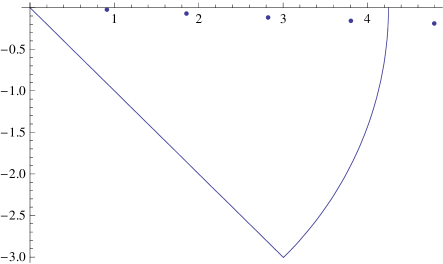
Figure 1: Integration contour in $k$-plane for $g=0.1$.

5 Time evolution for the unstable state

This is the central section of the paper, in which we compute the time evolution of unstable states by means of non-perturbative analytic techniques. The first problem is therefore that of defining an unstable particle and the second one to find the analog of such a state in our model. In physical terms, an unstable particle (or resonance) is related to the enhancement of any cross section producing that particle in the $s$-channel in a narrow band of $P^{2}\approx M^{2}$, where $P_{\mu}$ is the total 4-momentum and $M$ the particle mass. An unstable particle is therefore a quantum (i.e. coherent) state prepared at $t=0$, which is normalizable and has a non-trivial time evolution, not being an eigenstate of the system . In general, there is some freedom in the definition of such states. We try to keep as close a connection as possible with the procedure followed in perturbation theory: we take as unstable state an exact eigenstate of the non-interacting system ($g=0$), which is no more an exact eigenstate of the interacting system ($g\neq 0$). Let us then consider the evolution of a wave-function given at the initial time $t\,=\,0$ by

$$\psi^{(l)}(x,\,t=0)\,=\,\sqrt{\frac{2}{\pi}}\,\sin\left(l\,x\right)\,\theta(\pi-x)\,,$$ (32)

where $l$ is a positive integer. Note that, unlike the eigenfunctions $\psi_{k}(x)$ considered above, $\psi^{(l)}(x,0)$ is a normalized state:

$$\int_{0}^{\infty}\left|\psi^{(l)}(x,0)\right|^{2}\,dx\,=\,1\,.$$ (33)

Let us remark that any continuous wavefunction with support in the interval $(0,\pi)$ — representing the more general state for an unstable particle — can be expressed as superposition of the above wavefunctions. As discussed in the previous section, for $g=0$ the wavefunction above cannot decay being an eigenfunction and therefore we expect it to represent a slowly decaying state for $0<|g|\ll 1$. The decay products corresponds to non-normalizable wavefunctions in our model of the form

$$\phi_{k}(x,t)\,\propto\,\theta(x-\pi)\,\sin\big{[}k(x-\pi)\big{]}\,,$$ (34)

vanishing for $x\leq\pi$. For $g\neq 0$, also the wavefunctions above are not eigenfunctions; in physical terms, they can excite modes inside the cavity. The wavefunctions in eq. (32) exactly vanish outside the barrier, implying there are no “decay products” at $t=0$.

To compute the time evolution, namely

$$\psi^{(l)}(x,\,t)\,=\,e^{-i\hat{H}t}\,\psi^{(l)}(x,\,0)\,,$$ (35)

the most convenient technique is to expand the state above into eigenfunctions of the Hamiltonian which, as well known, have trivial time evolution:

$$\psi^{(l)}(x,\,0)\,=\,\int_{0}^{\infty}\varphi_{k}^{(l)}\,\psi_{k}(x)\,dk\,,$$ (36)

where:

$$\varphi^{(l)}_{k}\,=\,(-1)^{l}\,l\,\frac{2}{\pi}\,N_{k}(g)\,\frac{\sin k\pi}{k^{2}\,-\,l^{2}}\,,$$ (37)

satisfying $\varphi^{(l)}_{-k}=-\varphi_{k}^{(l)}$, with

$$N_{k}^{2}(g)\,=\,\frac{1}{4a_{k}b_{k}}\,=\,\frac{1}{1\,+\,1/(\pi gk)\sin 2k\pi\,+\,1/(2\pi^{2}g^{2}k^{2})(1-\cos 2k\pi)}\,.$$ (38)

We have considered for simplicity’s sake only the repulsive case $g>0$. Our wavefunction at time $t$ is therefore given by:

$$\psi^{(l)}(x,\,t)\,=\,\int_{0}^{\infty}\varphi^{(l)}_{k}\,\psi_{k}(x)\,e^{-i\,k^{2}\,t}\,dk\,.$$ (40)

5.1 Asymptotic Expansion of Wave Function

The spectral representation in eigenfunctions of the unstable state at time $t$ has the explicit expression:

$$~{}~{}~{}~{}~{}~{}~{}\psi^{(l)}(x,t)\,=\,\left(\frac{2}{\pi}\right)^{3/2}\int\limits_{0}^{\infty}p^{(l)}(k;x,g)\,e^{-ik^{2}t}\,dk,~{}~{}~{}~{}~{}~{}~{}0\,\leq\,x\,\leq\,\pi\,,~{}~{}~{}g\,>\,0\,,$$ (41)

where

$$p^{(l)}(k;x,g)\,=\,(-1)^{l}l\frac{\sin k\pi}{k^{2}-l^{2}}\,\frac{1}{1+1/(\pi gk)\sin 2k\pi+1/(2\pi^{2}g^{2}k^{2})(1-\cos 2k\pi)}\,\sin kx\,.$$ (42)

To obtain rigorous analytic formulae, we expand the integral for large $t$. The steepest descent method suggests to replace the integral on the r.h.s. of eq. (41) by the integral over the steepest descent ray ($0,\infty e^{-i\pi/4}$), on which the fast oscillation of the integrand is absent. This is achieved by computing the above integral over the sequence of closed contours $\gamma_{n}$ containing the segment on the real axis $(0,n+\alpha_{n})$, the ray $((n+\alpha_{n})e^{-i\pi/4},0)$ and a circular arc $c_{n}$ connecting the endpoints of the two segments (see fig. 1). The parameter $\alpha_{n}$ ($0\leq\alpha_{n}\leq 1/2)$ is chosen is such a way that $c_{n}$ passes at the maximal possible distance between the poles in the fourth quadrant of the $k$-plane. Therefore the state $\psi^{(l)}(x,t)$ is decomposed in a natural way into the sum of two quite different contributions:

$$\psi^{(l)}(x,t)\,=\,\psi^{(l)}_{pow}(x,t)\,+\,\psi^{(l)}_{exp}(x,t)\,,$$ (43)

where

$$\psi^{(l)}_{pow}(x,t) \equiv e^{-i\pi/4}\left(\frac{2}{\pi}\right)^{3/2}\,\int\limits_{0}^{\infty}p^{(l)}\left(k\,e^{-i\pi/4};x,g\right)\,e^{-k^{2}t}\,dk\,;$$ (44)

$$\psi^{(l)}_{exp}(x,t) \equiv -2\pi i\left(\frac{2}{\pi}\right)^{3/2}\sum_{n=1}^{\infty}{\rm Res}\left[p^{(l)}(k;x,g)\,e^{-ik^{2}t},\,k^{(n)}\right]\,.$$ (45)

In general, the contribution $\psi^{(l)}_{pow}(x,t)$ exhibits a power decay as $t\gg 1$, while the contribution $\psi^{(l)}_{exp}(x,t)$, coming from the residues in eq. (45), exhibits an exponential decay. Let us consider the above contributions in turn:

1. the integral $\psi^{(l)}_{pow}(x,t)$ is over the ray ($0,\,\infty\,e^{-i\pi/4}$) and for large $t\gg 1$ takes the dominant contribution from a neighborhood of $k=0$, where the integrand is analytic and can therefore be expanded in powers of $k$:

   $$p^{(l)}(k;x,g)\,=\,\frac{g^{2}}{(1+g)^{2}}\sum\limits_{j=1}^{\infty}p^{(l)}_{j}(x,g)\,k^{2j}\,.$$ (46)

   The first few coefficients explicitly read:

   $$p_{1}^{(l)}(x,g) = \frac{(-1)^{l+1}}{l}\,\pi x\,;$$ (47)

   $$p_{2}^{(l)}(x,g) = \frac{(-1)^{l+1}}{l}\pi x\left[\frac{1}{l^{2}}+\frac{\pi^{2}}{6}+\frac{2}{3}\frac{\pi^{2}g}{1+g}-\frac{\pi^{2}g^{2}}{(1+g)^{2}}-\frac{x^{2}}{6}\right]\,.$$ (48)

   Replacing this series into the integral and performing the change of variable $\nu=k^{2}\,t$, one obtains the following asymptotic expansion:

   $$\psi^{(l)}_{pow}(x,t) \approx \frac{\sqrt{2}}{\pi^{3/2}}\frac{e^{-i\pi/4}g^{2}}{(1+g)^{2}}\sum\limits_{j=1}^{\infty}\frac{(-i)^{j}\,p_{j}^{(l)}(x,v)}{t^{j+\frac{1}{2}}}\int\limits_{0}^{\infty}d\nu\,\nu^{j-\frac{1}{2}}\,e^{-\nu}$$ (49)

   $$= \frac{\sqrt{2}}{\pi}\frac{e^{-i\pi/4}g^{2}}{(1+g)^{2}}\sum\limits_{j=1}^{\infty}\frac{(-i)^{j}(2j-1)!!}{2^{j}}\frac{p_{j}^{(l)}(x,g)}{t^{j+\frac{1}{2}}},~{}~{}0\leq x\leq\pi,~{}t\gg 1,$$ (50)

   whose first few terms read:

   $$\psi^{(l)}_{pow}(x,t) \approx \frac{e^{i\pi/4}}{\sqrt{2}}\frac{(-1)^{l}}{l}\frac{g^{2}}{(1+g)^{2}}\frac{x}{t^{3/2}}\Bigg{\{}1\,-\,\frac{3i}{2t}\Bigg{[}\frac{1}{l^{2}}+\frac{\pi^{2}}{6}+\frac{2}{3}\frac{\pi^{2}g}{1+g}\,+$$ (51)

   $$~{}~{}~{}~{}~{}~{}~{}~{}~{}~{}~{}~{}~{}~{}~{}~{}~{}~{}~{}~{}~{}~{}~{}~{}~{}~{}~{}~{}~{}~{}~{}~{}~{}~{}~{}-\frac{\pi^{2}g^{2}}{(1+g)^{2}}-\,\frac{x^{2}}{6}\Bigg{]}+\mathcal{O}\left(\frac{1}{t^{2}}\right)\Bigg{\}}\,.$$

   Let us make a few remarks. The above asymptotic expansion is uniformely valid for all $g\geq 0$, since the coefficients $p_{j}^{(l)}(x,g)$ are uniformely bounded in that region (see eq. (46)). The exponent $3/2$ controlling the power decay, $\psi\approx 1/t^{3/2}$, does not depend on $l$ and $g$;

2. the simple poles $k^{(n)}(g)$ of the integrand in $\psi_{exp}^{(l)}(x,t)$ are the simple zeroes of the trascendental equation

   $$4a_{k}b_{k}\,=\,1+\frac{\sin 2k\pi}{\pi gk}+\frac{1-\cos 2k\pi}{2\pi^{2}g^{2}k^{2}}\,=\,0\,,$$ (52)

   constrained by the conditions:

   $$\mathrm{Re}\,k^{(n)}\,>\,|\mathrm{Im}\,k^{(n)}|\,,~{}~{}~{}\mathrm{Im}\,k^{(n)}\,<\,0\,.$$ (53)

   It is easy to prove that all the poles $k^{(n)}(g)$ satisfy all of the above conditions for $g\ll 1$. The second condition in (53) is always satisfied. In general, the poles leave the fourth quadrant for very large values of $|g|$, where the unstable-particle description is irrelevant.

   

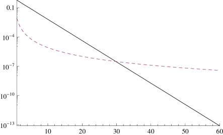
   Figure 2: Time evolution of the modulus square of the exponential contribution (continuous line) and power contribution (dashed line) to the wavefunction of the fundamental state $l=1$ (see eq.(32)) for $g=0.2$, integrated in the interval $(0,\pi)$. The scale on the vertical axis is logarithmic.

   The unstable states (or resonances) have pole contributions for $g\ll 1$ of the form:

   $$\psi_{exp}^{(l)}(x,t)\,=\,\psi_{pole}^{(l)}(x,t)\,+\,g\sum_{n\,\neq\,l}^{1,\,\infty}\,c_{\,l,\,n}\,\psi_{pole}^{(n)}(x,t)\,,$$ (54)

   where

   $$c_{\,l,\,n} \equiv (-1)^{l+n}\frac{2\,l\,n}{l^{2}-n^{2}}\,;$$ (55)

   $$\psi_{pole}^{(n)}(x,t) \equiv \sqrt{\frac{2}{\pi}}\,Z^{(n)}(g)\,\sin\left[k^{(n)}(g)x\right]\,e^{-i\,\omega^{(n)}(g)\,t-1/2\,\Gamma^{(n)}(g)\,t}\,,$$ (56)

   with

   $$Z^{(n)}(g) = 1-\frac{g}{2}\,+\mathrm{O}\left(g^{2}\right)\,;$$ (57)

   $$\omega^{(n)}(g) \equiv +\,\left(\mathrm{Re}\,k^{(n)}\right)^{2}\,-\,\left(\mathrm{Im}\,k^{(n)}\right)^{2}$$ (58)

   $$= n^{2}\left[1-2g\,+\mathrm{O}\left(g^{2}\right)\right]\,;$$

   $$\Gamma^{(n)}(g) \equiv -\,4\,{\mathrm{Re}\,k^{(n)}}\,{\mathrm{Im}\,k^{(n)}}$$ (59)

   $$= 4\pi n^{3}g^{2}\left[1\,-\,4g\,+\,{\mathcal{O}}\left(g^{2}\right)\right]\,.$$

6 Discussion

Let us consider the asymptotic expansion for $t\gg 1$ of the first resonance ($l=1$) by neglecting the contributions of the higher-order poles ($n>1$):

$$\psi^{(1)}(x,t) \approx -\frac{e^{i\pi/4}}{\sqrt{2}}\frac{g^{2}}{(1+g)^{2}}\frac{x}{t^{3/2}}\left\{1\,-\,\frac{3i}{2t}\,\Bigg{[}1+\frac{\pi^{2}}{6}+\frac{2}{3}\frac{\pi^{2}g}{1+g}\,-\frac{\pi^{2}g^{2}}{(1+g)^{2}}-\,\frac{x^{2}}{6}\Bigg{]}+\mathcal{O}\left(\frac{1}{t^{2}}\right)\right\}+$$ (60)

$$+ \sqrt{\frac{2}{\pi}}\left(1-\frac{g}{2}\right)\,\sin\left[\left(1-g\right)x\right]\,\exp\left[-i\left(1-2g\right)t\,-\,2\pi g^{2}t\right]\,.$$

A few comments are in order:

1. in the limit $g\to 0$, the power term disappears from the r.h.s. of eq. (60) and the exponential term approaches the fundamental eigenfunction of a particle with mass $m=1/2$ in a box of length $l=\pi$:

   $$\Psi^{(1)}(x,t)\,\to\,\sqrt{\frac{2}{\pi}}\,\sin x\,e^{-i\,t}\,,~{}~{}~{}~{}g\to 0\,.$$ (61)

   That is in complete agreement with physical intuition, as already discussed;

2. it is clear that, for sufficiently long times, the decay law will be dominated by the power term. However, since the power term has a small coefficient, suppressed as $g^{2}\ll 1$ for small $g$, while the exponential term has a coefficient of order one and it remains $\mathcal{O}(1)$ as long as $t\raisebox{-3.0pt}{$\>\stackrel{{\scriptstyle<}}{{\scriptstyle\sim}}\>$}1/g^{2}$, the exponential term dominates over the power term for a large temporal region for $g\ll 1$. In other words, if $g$ is small and $t$ is large, but such that

   $$1\,\ll\,t\,\raisebox{-3.0pt}{$\>\stackrel{{\scriptstyle<}}{{\scriptstyle\sim}}\>$}\,\,\frac{\log(1/g)}{g^{2}}\,,$$ (62)

   there is a long transient in which the exponential term prevails on the power term (see fig. 2). Since the signal rapidly decays with time, the transient region may actually be the one measurable one.

Acknowledgements

One of us (U.G.A.) would like to thank D. Anselmi and M. Testa for discussions.

NOTE ADDED

After the first version of this note was put on the archive, references [7] and [8] were brought to our attention. While the first paper deals with general properties of the exponential region, the second one treats the time evolution with the saddle point method of the same model as we do. We are in complete agreement with [8] as far as the asymptotic power behavior in time is concerned, while we are in disagreement with the exponential behavior. More specifically, the first term on the r.h.s. of our eq.(54), i.e. the diagonal one $n=l$, is in agreement with the r.h.s. of eq.(2a) in [8] ($l$ labels the initial state and $n$ the pole). In [8] however, the non-diagonal pole contributions $n\neq l$, present in eq.(54), are not included. These terms have a coefficient suppressed by a power of $g\ll 1$ compared to the diagonal one, but have a slower exponential decay for $n<l$ ($\Gamma^{(n)}\propto n^{3}$, see eq.(59)), and therefore dominate at intermediate times (i.e. before power-effects take over). As shown in fig.3, there is indeed a large temporal region where the non-diagonal contribution from the first pole,

$$\frac{16}{9}g^{2}\int_{0}^{\pi}|\psi_{pole}^{(1)}(x,t)|^{2}dx\,,$$ (63)

dominates over that of the second pole,

$$\int_{0}^{\pi}|\psi_{pole}^{(2)}(x,t)|^{2}dx\,,$$ (64)

in the temporal evolution of the first excited state, $l=2$. Neglecting the non-diagonal contributions is therefore a reasonable approximation only for the time-evolution of the lowest-lying state $l=1$. More details will be given in a forthcoming publication [9].

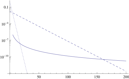
Figure 3: Time evolution of the contributions to the $l=2$, i.e. first excited, state for $g=0.1$. Dotted line: second pole contribution; Dashed line: first pole contribution; Continuous line: power contribution.

References

- [1] R. P. Feynman, La Fisica di Feynman (The Feynman Lectures in Physics), Masson Italia Editori, Milano (1985), vol. 3.
- [2] A. Degasperis and L. Fonda, Does the life-time of an Unstable Particles Depend on the Measuring Apparatus?, Il Nuovo Cimento vol. 21, n. 3 (1974).
- [3] L. Maiani and M. Testa, Unstables Systems in Relativistic Quantum Field Theory, Ann. of Phys. vol. 263, n. 2, pag. 353 (1998).
- [4] See for example: E. Segre, Nuclei e Particelle, Zanichelli Ed. (1982), chap. 7.
- [5] S. Flugge, Practical Quantum Mechanics, Springer-Verlag, Berlin (1994), problem n. 27.
- [6] R. Newton, Scattering of Waves and Particles, Dover Publications, Inc. Mineola, New-York (2004); M. Goldberger and K. Watson, Collision Theory, Dover Publications, Inc. Mineola, New-York (2002).
- [7] N. Hatano et al, Prog. Theor. Phys. Vol. 119 n.2 pag. 187 (2008) and references therein.
- [8] R. G. Winter, Phys. Rev. 123, 1503 (1961).
- [9] U.G. Aglietti and P.M. Santini, in preparation.