A semi-analytical approach to perturbations in mutated hilltop inflation

Abstract

We study cosmological perturbations and observational aspects for mutated hilltop model of inflation. Employing mostly analytical treatment, we evaluate observable parameters during inflation as well as post-inflationary perturbations. This further leads to exploring observational aspects related to Cosmic Microwave Background (CMB) radiation. This semi-analytical treatment reduces complications related to numerical computation to some extent for studying the different phenomena related to CMB angular power spectrum for mutated hilltop inflation.

I introduction

The most striking aspect of cosmological inflationary scenario guth is that they provide natural explanation for the origin of cosmological perturbation seeds for structure formation leading to a nearly scale-free power spectrum which is in tune with direct observational evidence from Cosmic Microwave Background Radiation (CMB) wmap3 ; wmap07 and Large Scale Structure Formation large . The form of the primordial perturbations seems to explain the observed temperature anisotropy in the CMB wmap3 ; wmap07 .

Recently we have proposed a variant of hilltop inflation, namely, mutated hilltop inflation barun , in order to explain the early universe. The analytical expressions for most of the observable parameters have been obtained. However, as pointed out in that paper, the expression for the ratio of the tensor to scalar amplitudes does not exactly conform with the usual consistency relation $r=-8n_{T}$ andrew . In the present article, we have tried to search for a possible explanation for the same by deviating slightly from perfect de-Sitter approximation right from the beginning. This turns out to be a complimentary approach of the previously employed approaches of obtaining modified consistency relation, such as, when higher order terms of the slow roll parameters are taken into account stewart ; 0101225 ; PRD66 , if tensor to scalar ratio is expressed as a function of tensor spectral index, scalar spectral index and running of the tensor spectral index parker , if generalized propagation speed (less than one) of the scalar field fluctuations relative to the homogeneous background is considered peiris ; bean ; mukhanov and the likes.

The advent of highly precise data from the observational probes like COBE cobe , WMAP wmap3 and the forthcoming Planck planck has made the task for the development of the framework of post-inflationary perturbation more difficult in order to met up with challenges both from building up a theoretical framework of post-inflationary perturbative technique and from confronting the theory with observations more precisely. This usually leads to employ direct numerical techniques by exploiting highly sophisticated numerical codes like CAMB camb . Of course, one has to rely on numericals at some point while performing data analysis from WMAP wmap3 but it is always better to see how far one can go analytically, which may sometime lead to deeper physical insight as well. This is the primary motivation for employing semi-analytical treatment for perturbations in our typical model of inflation, viz. mutated hilltop inflation. To this end, we mostly employ the framework of post-inflationary perturbations developed by Mukhanov (for an useful review see mukhanovb ) and obtain analytical results for CMB power spectrum for our typical model. This will in turn help us reduce numerical complications to a great extent for our model.

II Quantum fluctuation and origin of inhomogeneities

The standard theory of cosmological perturbations is based on the formalism developed in barun38 . To study the quantum fluctuations and subsequent classical perturbations for mutated hilltop inflation let us directly refer to barun where the inflationary potential has the following form

$$V(\phi)=V_{0}\left[1-{\rm sech}(\alpha\phi)\right]$$ (1)

This represents a single scalar field driven inflationary potential and falls in the wider class of hilltop inflation hilllyth1 .

II.1 Curvature perturbation

The expression for comoving curvature perturbation is acquired by solving the well known Mukhanov-Sasaki equation mukhanov1sasaki and in the slow-roll approximation we obtain

$${\cal R}_{k}\approx-\frac{\alpha\sqrt{V_{0}}}{M_{P}\sqrt{3}}\frac{|\eta|e^{-ik\eta}}{\sqrt{2k}}\left(1-\frac{i}{k\eta}\right)A(\eta)$$ (2)

where $A(\eta)\equiv\ln\left(a_{1}M_{P}^{-1}\sqrt{\frac{V_{0}}{3}}|\eta|\right)$. Therefore the dimensionless spectrum for ${\cal R}_{k}$ turns out to be

$$P_{\cal R}(k)=\frac{\alpha^{2}V_{0}}{12\pi^{2}M_{P}^{2}}(1+k^{2}\eta^{2})A(\eta)^{2}$$ (3)

Evaluating the spectrum at horizon crossing, using the de-Sitter approximation $k=aH=-\eta^{-1}$ we obtain

$$P_{\cal R}(k)|_{k=aH}=\frac{\alpha^{2}V_{0}}{6\pi^{2}M_{P}^{2}}A(\eta)^{2}$$ (4)

But in adopting exact de-Sitter relation at horizon crossing we are discarding the effect of the evolution of the scalar field. In what follows we shall pursue a non trivial path. We first note that for the inflation model under consideration at the time of horizon crossing,

$$1+k^{2}\eta^{2}\approx 2-\frac{1}{\alpha^{2}\sqrt{\frac{V_{0}}{3}}M_{P}(d-t)}$$ (5)

which is slightly different from the usual de-Sitter relation $1+k^{2}\eta^{2}=2$. Eqn.(5) shows that there will be direct effect of the evolution of the scalar field on the observable parameters when they are evaluated at horizon exit. Our approach is a bit similar to peiris , where variable speed of the scalar field fluctuations have been taken into account for evaluating observable quantities at horizon exit. Following this trail the power spectrum turns out to be

$$P_{\cal R}|_{k=aH}=\frac{\alpha^{2}V_{0}}{12\pi^{2}M_{P}^{2}}\left[2-\frac{\alpha^{-2}M_{P}^{-2}}{A(\eta)}\right]A(\eta)^{2}$$ (6)

Comparison of the Eqns.(4) and (6) shows that the correction term indeed has some significant role from theoretical aspects. We may now re-derive all the allied expressions for the observable quantities in a more accurate way. The expression for the scalar spectral index is now given by

$$n_{s}=1-\left[\frac{4A(\eta)-\alpha^{-2}M_{P}^{-2}}{2A(\eta)^{2}-\alpha^{-2}M_{P}^{-2}A(\eta)}\right]$$ (7)

We have also succeeded in calculating the running of the spectral index which turns out to be

$$\frac{dn_{s}}{d\ln k}{\displaystyle\left|{}_{k=aH}\right.}=-\left[\frac{8A(\eta)^{2}-4\alpha^{-2}M_{P}^{-2}A(\eta)+\alpha^{-4}M_{P}^{-4}}{\left(2A(\eta)^{2}-\alpha^{-2}M_{P}^{-2}A(\eta)\right)^{2}}\right]$$ (8)

Clearly, though the quantity within the parentheses is quite small still gives a nonzero value resulting in a negative running of the spectral index consistent with WMAP3 data set.

II.2 Tensor fluctuation

The tensor modes representing primordial gravitational waves, obtained in a similar way as the scalar modes and the corresponding spectrum is given by

$$P_{T}|_{k=aH}=\frac{V_{0}}{3\pi^{2}M_{P}^{4}}\left[2-\frac{\alpha^{-2}M_{P}^{-2}}{A(\eta)}\right]$$ (9)

As expected, the spectrum for the tensor modes is also modified in this approach. The corresponding spectral index turns out to be

$$n_{T} = -\frac{1}{\alpha^{2}M_{P}^{2}}\left[\frac{1}{2A(\eta)^{2}-\alpha^{-2}M_{P}^{-2}A(\eta)}\right]$$ (10)

From Eqns.(9) and (6) we arrive at the expression for the ratio of tensor to scalar amplitudes, given by

$$r = 4\frac{\alpha^{-2}M_{P}^{-2}}{A(\eta)^{2}}$$ (11)

We shall use this expression in calculating $r$ and subject it to observational verification ($r<0.1$) wmap07 .

Combining Eqns.(11) and (10) we obtain a vital relation between tensor spectral index $n_{T}$ and the tensor to scalar amplitude ratio $r$ as,

$$r=-8n_{T}\left(1-\frac{\sqrt{r}}{4\alpha M_{P}}\right)$$ (12)

The spectrum $P_{T_{|_{k=aH}}}$ of tensor perturbation conveniently specified by the tensor fraction $r=\frac{P_{T}{|_{k=aH}}}{P_{\cal R}{|_{k=aH}}}$ yields the relation $r=-8n_{T}$ in the slow-roll approximation andrew ; david1 . But Eqn.(12) shows that when the explicit effect of the scalar field evolution is taken into account in evaluating the observable parameters at horizon exit we obtain a consistency relation which is slightly modified. Of course, there exist in the literature other ways of obtaining a modified consistency relation. Such a modified consistency relation can be found in any analysis where higher order terms in the expansion of slow roll parameters are taken into account 0101225 ; PRD66 . The consistency relation is also modified in the context of brane inflation peiris ; bean and non-standard models of inflation (mukhanov, ) where generalized propagation speed (less than one) of the scalar field fluctuations relative to the homogeneous background have been considered. Further, deviation from the usual consistency relation can be found in (parker, ) where tensor to scalar ratio has been shown to be a function of tensor spectral index, scalar spectral index and running of the tensor spectral index. Our approach is somewhat similar to these.

Finally, we estimate the observable parameters from the first principle of the theory of fluctuation as derived in this section for three sets of values of $\alpha$ and tabulate it in Table 1.

$\alpha$	$a_{1}$	$P_{R}^{1/2}$	$n_{s}$	$r$
$M_{P}^{-1}$	$M_{P}^{-1}$
$2.9$	$6.7091\times 10^{25}$	$3.77624\times 10^{-5}$	0.96088	$1.81759\times 10^{-4}$
$3.0$	$6.6492\times 10^{25}$	$3.90592\times 10^{-5}$	0.96088	$1.69903\times 10^{-4}$
$3.1$	$6.5945\times 10^{25}$	$4.03766\times 10^{-5}$	0.96087	$1.59170\times 10^{-4}$

Table 1: Table for the observable quantities as obtained from the theory of fluctuations

From the table it is quite clear that the observable parameters related to perturbations, are in excellent agreement with observational data.

III Post-inflationary evolution of perturbations

Now to relate the initial perturbation seeds with cosmological observables we study post-inflationary evolution of these perturbation proceeding analytically as far as possible from our specific model.

While a perturbation mode re-enters the horizon during matter dominated era, we obtain the approximate solution for the fluctuations in the gravitational potential from the relation

$$\Phi_{k} \approx -\frac{3}{5}{\cal R}_{k}$$ (13)

It should be pointed out that Eqn.(13) is an approximate solution for the gravitational potential so that we can neglect contributions from smaller scales spatial gradient. Still qualitative information about the evolution of $\Phi$ in the large scale regime is transparent. Using the near constancy of ${\cal R}_{k}$ in the superhorizon scales malik , we obtain an approximated expression for the comoving curvature perturbation and for our typical model at horizon reentry during matter domination this turns out to be

$${\cal R}_{k}\simeq\frac{\alpha}{M_{P}}\sqrt{\frac{V_{0}}{3}}\frac{i}{\sqrt{2k^{3}}}B(k)$$ (14)

where $B(k)\equiv\ln\left(2a_{1}M_{P}^{-1}{\sqrt{\frac{V_{0}}{3}}}k^{-1}\right)$. So the fluctuation modes of the gravitational potential, entering the horizon during the matter dominated era, are given by,

$$\Phi|_{k=aH}\approx-\frac{3\alpha}{5M_{P}}\sqrt{\frac{V_{0}}{3}}\frac{i}{\sqrt{2k^{3}}}B(k)$$ (15)

From the above expression it is apparent that in this model the gravitational potential is not strictly scale invariant, but has a slight scale dependence with a mild running as expected.

Using Eqn.(15), the spectrum of the matter density contrast can be found from Poisson equation, turns out to be

$$P_{\delta}|_{k=aH}\approx\frac{16\alpha^{2}V_{0}}{75\pi^{2}M^{2}_{P}}B(k)^{2}$$ (16)

and the corresponding spectral index and the running are respectively given by

$$n_{\delta}\approx 1-2B(k)^{-1},~{}n^{{}^{\prime}}_{\delta}\approx-2B(k)^{-2}$$ (17)

Eqn.(17) shows that the spectral index is not exactly scale invariant, it has a small negative tilt with negative running.

The fluctuations produced during inflation are scale dependent as is evidenced in Section II and this is reflected in the matter spectrum. As a consequence, we obtain negative scalar spectral tilt and negative running of the scalar spectral index for the matter power spectrum for our model.

IV Temperature anisotropies in CMB

Let us now proceed further with the analytical treatment and discuss the CMB angular power spectrum resulting from temperature anisotropies due to scalar curvature perturbations for our typical inflationary model. The dominant contribution to the large scale CMB anisotropy comes from the Sachs-Wolfe effect sachs . In the sudden decoupling approximation for adiabatic perturbation, the assumption of complete matter domination at last scattering provide us the Sachs-Wolfe spectrum for the typical model of our consideration, which is approximately given by

$$C^{\mbox{SW}}_{l}\approx\frac{\alpha^{2}V_{0}}{75\pi M^{2}_{P}}\left(\ln\left[a_{1}M^{-1}_{P}\sqrt{\frac{V_{0}}{3}}\frac{2\eta_{0}}{l}\right]\right)^{2}\frac{1}{2l(l+1)}$$ (18)

Here $\eta_{0}$ is the present dimensionless comoving distance to the last scattering surface.

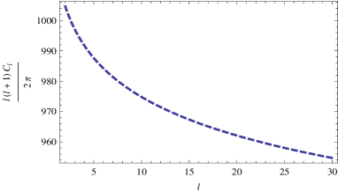
Figure 1: Sachs-Wolfe plateau

Figure 1 shows variation of angular power spectrum for Sachs-Wolfe effect $\frac{l(l+1)}{2\pi}C^{SW}_{l}$ with the CMB multipoles $l$ in units of $\mu K^{2}$, where we have taken the following representative values for the quantities involved: $V_{0}^{1/4}=1.4\times 10^{-3}M_{P}$, $\alpha=3.0M_{P}^{-1}$, $a_{1}=6.6492\times 10^{25}M_{P}^{-1}$ and $\eta_{0}=7.42438\times 10^{26}$. Figure 1 reveals that the Sachs-Wolfe plateau is not exactly flat but is slightly tilted towards larger values of $l$. This is not surprising, since the primordial curvature perturbation in mutated hilltop inflation is not strictly scale-invariant.

In the smaller scales CMB spectrum is dominated by acoustic oscillation of the baryon-photon fluid. The approximate solution to the acoustic oscillation equation lythR ; liddlelyth for our case turns out to be

$$\frac{1}{4}\delta_{\gamma k}\approx-(1+R)\Phi_{k}+\frac{1}{2}T^{0}_{k}\Phi^{0}_{k}\cos(kr_{s})$$ (19)

where $r_{s}\equiv\int^{\eta}_{0}c_{s}(\eta)d\eta$, $c_{s}$ is the sound speed, $R=\frac{3\rho_{b}}{4\rho_{\gamma}}$, $\Phi_{k}\equiv-\frac{3}{5}T_{k}{\cal R}_{k}$ is the small scale solution of the gravitational potential with $T_{k}$ being corresponding transfer function and we have defined

$$\Phi^{0}_{k}\equiv-\frac{2\alpha}{3M_{P}}\sqrt{\frac{V_{0}}{3}}\frac{1}{\sqrt{2k^{3}}}\left[\ln\left(a_{1}M_{P}^{-1}{\sqrt{\frac{V_{0}}{3}}}k^{-1}\right)\right]$$ (20)

to be the initial gravitational potential fluctuation and $T^{0}_{k}$ is the associated transfer function. The expression for the photon velocity perturbation $V_{\gamma k}$ is then given by

$$V_{\gamma k}\approx\frac{3c_{s}}{2}T^{0}_{k}\Phi^{0}_{k}\sin(kr_{s}).$$ (21)

So the CMB angular power spectrum for our typical model turns out to be mukhanovb

$$C_{l}\approx 4\pi P_{\Phi^{0}}\int^{\infty}_{0}\left[C-D\cos(\rho lx)+E\cos^{2}(\rho lx)+F\left(1-\frac{l(l+1)}{l^{2}x^{2}}\right)\sin^{2}(\rho lx)\right]j^{2}_{l}(xl)\frac{dx}{x}$$ (22)

here $x=\frac{k\eta_{0}}{l}$, and the functions in the integrand are defined as follows:

$$C \equiv \frac{81}{100}R^{2}{T}^{2}(x)e^{-\frac{l^{2}x^{2}}{l^{2}_{f}}},~{}D\equiv\frac{9}{10}RT(x)T^{0}(x)e^{-1/2\frac{l^{2}x^{2}}{l^{2}_{f}+l^{2}_{s}}},~{}E\equiv\frac{1}{4}{T^{0}}^{2}(x)e^{-\frac{l^{2}x^{2}}{l^{2}_{s}}},~{}F\equiv\frac{9}{4}c^{2}_{s}{T^{0}}^{2}(x)e^{-\frac{l^{2}x^{2}}{l^{2}_{s}}},$$

$$~{}l^{-2}_{f} \equiv 2\sigma^{2}(\frac{\eta_{LS}}{\eta_{0}})^{2},~{}l^{-2}_{s}\equiv 2\left[\sigma^{2}+(k_{D}\eta_{Ls})^{-2}\right](\frac{\eta_{LS}}{\eta_{0}})^{2},~{}\rho\equiv\frac{1}{\eta_{0}}\int^{\eta_{LS}}_{0}c_{s}d\eta,~{}\sigma\equiv 1.49\times 10^{-2}\left[1+\left(1+z_{EQ}/z_{LS}\right)^{-1/2}\right]$$

with $z_{EQ}~{}\mbox{ and }~{}z_{LS}$ are redshifts corresponding to matter-radiation equality and last scattering surface respectively and $k^{-2}_{D}\equiv\left[\frac{2}{5}\int^{\eta}_{0}c^{2}_{s}\frac{\tau_{\gamma}}{a}d\eta\right]$, is the Silk damping scale silk ; liddlelyth ; dodelson . Here $\tau_{\gamma}$ is the mean free time for photon scattering and “LS” stands for last scattering. The slight scale dependence of the primordial curvature perturbation is reflected here via

$$P_{\Phi^{0}}\equiv\frac{\alpha^{2}V_{0}}{27\pi^{2}M^{2}_{P}}\left[\ln\left(a_{1}M_{P}^{-1}{\sqrt{\frac{V_{0}}{3}}}~{}\frac{\eta_{0}}{l}\right)\right]^{2}$$ (23)

The results we have obtained may not be exact, but still qualitative behavior of the associated physical quantities can be extracted from them very easily.

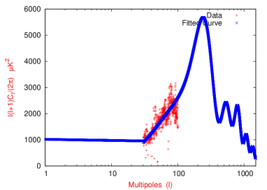
Figure 2: The total CMB angular power spectrum for adiabatic modes

To analyze the entire CMB angular power spectrum, we shall concentrate on Figure 2 which depicts its behavior for the entire significant range of the multipoles ($1\leq l\leq 1500$) and combines almost all the effects arising in CMB. Figure 2 can be split into 3 regions: (i) $1\leq l\leq 30$ represents mainly Sachs-Wolfe effect, (ii) for $30<l\leq 100$ we have considered the exact expression for the Bessel function in Eqn.(22) and finally (iii) for $100<l\leq 1500$ large $l$ limit of the Bessel function has been used for a rigorous calculation of the CMB spectrum. For the plots we have used the transfer functions from mukhanovb with appropriate modifications: $T^{0}(x)=1.20+0.09\ln\left(\frac{I_{\Lambda}l~{}x}{250\sqrt{\Omega_{m}}}\right)$ and $T(x)=0.52-0.21\ln\left(\frac{I_{\Lambda}l~{}x}{250\sqrt{\Omega_{m}}}\right)$; where the late time effects due to dark energy have been incorporated via $I_{\Lambda}$ which is defined as $I_{\Lambda}\equiv 3\left(\frac{\Omega_{\Lambda}}{\Omega_{M}}\right)^{\frac{1}{6}}\left[\int^{\sinh^{-1}\sqrt{\Omega_{\Lambda}/\Omega_{M}}}_{0}\frac{dx}{(\sinh x)^{2/3}}\right]^{-1}$.

In Figure 2 resulting from our analysis the first and the most prominent peak of the acoustic oscillation arises at $l\approx 241$ and at a height of $\approx 5900\mu K^{2}$. The first peak is followed by two nearly equal height peaks at $l\approx 533$ and $791$. After the third peak there is a damping tail in the oscillation with successive peaks with lower heights. This happens due to considering Silk damping effect in our analysis, which is also consistent with CMB observations. So mutated hilltop inflation conform well with the recent observations.

V Summary and Discussions

In this article we have studied quantum fluctuations and corresponding classical perturbations as well as allied observational aspects by a semi-analytical treatment, based on mutated hilltop model of inflation. We have succeeded in deriving analytical expressions for most of the observable parameters. An approximated expression for the fluctuations in the gravitational fluctuations has also been successfully obtained using relativistic perturbations. We have also obtained an expression for the scale dependent matter power spectrum, along with a negative running of the corresponding spectral index which are in accord with recent observational demands. We have shown explicitly that in mutated hilltop inflation the Sachs-Wolfe plateau is not strictly flat but is slightly tilted towards the larger multipoles. Moreover, we have also studied the baryon acoustic oscillation based on our model by carrying the analytical framework as far as possible, which gives physical insight to the scenario and reduces numerical complications to a great extent. Finally, we have employed certain simplistic numerical techniques and found that the positions of the acoustic peaks conform well within the estimated values of different cosmological parameters.

Some comments on employing this semi-analytical treatment to mutated hilltop inflation model are in order. The resulting CMB power spectrum as obtained from our analysis is quite consistent with what can be obtained from direct numerical techniques via CAMB camb . Of course, using more complicated numerical technique via Monte-Carlo simulation like COSMOMC cosmomc will result in more accurate estimation of individual cosmological parameters but, at a first go, this semi-analytical approach is more or less sufficient for extracting physics out of our typical model. In future we would like to employ COSMOMC to our model as a complimentary techniques of extracting physics out of mutated hilltop inflation model.

References

- (1) A. H. Guth, Phys. Rev. D23, 347 (1981)
- (2) M. Tegmark et. al., Phys. Rev. D 69, 103501 (2004)
- (3) WMAP collaboration, D. N. Spergel et al., Astrophys. J. Suppl. 170, 377 (2007); for uptodate results on WMAP, see http://lambda.gsfc.nasa.gov/product/map/current
- (4) T. Padmanabhan, Theoretical Astrophysics, Volume III: Galaxies and Cosmology, Cambridge University Press, U. K. (2002)
- (5) B. K. Pal, S. Pal and B. Basu, JCAP 1001, 029 (2010)
- (6) A. R. Liddle and D. H. Lyth, Phys. Lett. B 291, 391 (1992)
- (7) E. D. Stewart and D. H. Lyth Phys. Lett. B 302, 171 (1993)
- (8) Ewan D. Stewart and Jin-Ook Gong, Phys. Lett. B 510, 1 (2001)
- (9) Eckehard W. Mielke and Humberto H. Peralta, Phys. Rev. D 66, 123505 (2002)
- (10) I. Agullo et al. Gen. Rel. Grav. 41, 2301 (2009)
- (11) H. V. Peiris et al., Phys. Rev. D76, 103517 (2007)
- (12) R. Bean et al., JCAP 0705 004 (2007)
- (13) J. Garriga and V. F. Mukhanov, Phys. Lett. B458, 219 (1999)
- (14) G. F. Smoot et al., Astrophys. J. 396, L1 (1992); S. Dodelson and J. M. Jubas, Phys. Rev. Lett. 70, 2224 (1993)
- (15) Planck collaboration, http://www.rssd.esa.int/index.php?project=Planck; P. A. R. Ade et.al., arxiv:1101.2022
- (16) Online link: http://camb.info/
- (17) V. F. Mukhanov, Physical Foundation of Cosmology, Cambridge University Press, U.K.(2006)
- (18) V. F. Mukhanov and G. V. Chibisov, JETP Lett. 33, 532 (1981); S. W. Hawking, Phys. Lett. B 115, 295 (1982); A. A. Starobinsky, Phys. Lett. B 117, 175 (1982); A. H. Guth and S. Y. Pi, Phys. Rev. Lett. 49, 1110 (1982)
- (19) L. Boubekeur and D. H. Lyth, JCAP 0507, 010 (2005); K. Kohri, C.-M. Lin and D. H. Lyth, JCAP 0712, 004 (2007)
- (20) V. F. Mukhanov, JETP Lett. 41 493 (1986); M. Sasaki, Prog. Theor. Phys. 76, 1036 (1986)
- (21) A. R. Liddle and D. H. Lyth, Phys. Rep. 231, 1 (1993)
- (22) D. H. Lyth, K. A. Malik, M. Sasaki, JCAP 0505 004 (2005)
- (23) R. K. Sachs and A. M. Wolfe, Astrophys. J. 147, 73 (1967)
- (24) D. H. Lyth, Phys. Rev. D31, 1792(1985); W. Hu and M. Sugiyama, Astrophys. J. 471, 542 (1996);
- (25) D. H. Lyth and A. R. Liddle, The Primordial Density Perturbation, Cambridge University Press, U.K.(2009)
- (26) J. Silk, Nature 215, 1155 (1972)
- (27) S. Dodelson, Modern Cosmology, Academic Press, USA (2003)
- (28) http://cosmologist.info/cosmomc/