Spontaneous symmetry breaking: variations on a theme

Abstract

Spontaneous symmetry breaking (SSB) is a widespread phenomenon in several areas of physics. In this paper I wish to illustrate some situations where spontaneous symmetry breaking presents non obvious aspects. The first example is taken from molecular physics and is related to the paradox of existence of chiral molecules. The second case refers to a Dirac field in presence of a magnetic field. Gusynin, Miransky and Shovkovy have shown that Nambu–Jona-Lasinio (NJL) models, where SSB of chiral symmetry takes place for the nonlinear coupling over a certain threshold, in presence of a magnetic field exhibit SSB for any value of the coupling. They called this phenomenon magnetic catalysis. I will discuss this problem in $2+1$ dimensions from an operatorial point of view and show that the basic phenomenon is a double pairing induced by the magnetic field in the vacuum for any value of the mass. This pairing provides the environment responsible for chiral symmetry breaking in NJL models with very weak nonlinearities. The third case illustrates briefly SSB in stationary nonequilibrium states and its possible relevance in natural phenomena.

1 Introduction

The problems considered in this paper have a previous history in the literature. Here, after a brief review, we shall elaborate on their interpretation and significance.

The first problem refers to molecular physics, more precisely to the existence of chiral molecules, that is molecules that rotate the polarization of light. Hund was the first to point out in 1927 that such molecules according to quantum mechanics should not exist as the corresponding Hamiltonian is invariant under mirror reflection [1]. This problem became known as the Hund’s paradox and was discussed in the physico-chemical literature for decades.

In the following we shall argue that SSB provides a solution to the paradox once we take into account that the experiments deal with a large number of molecules and that their interactions are sufficient to keep them in the chiral state. This idea was behind work done previously in collaborations with Pierre Claverie [2], Carlo Presilla and Cristina Toninelli [3], but was not completely explicit as the emphasis was on instabilities that set in at the semiclassical limit and localization phenomena. We will mention also a complementary point of view proposed by other authors.

The second case refers to a quantum Dirac field in $2+1$ dimensions in presence of a magnetic field orthogonal to the plane where the particles live. This system is invariant under chiral gauge transformations in the limit of vanishing mass. Gusynin, Miransky and Shovkovy [4] pointed out that in a NJL model [6] in $2+1$ dimensions in presence of a magnetic field a finite mass is produced, that is chiral SSB takes place, for any value of the nonlinear coupling. In other words there is no threshold as it happens in absence of magnetic field. They showed that the same happens in $3+1$ dimensions [5]. They called this phenomenon magnetic catalysis and explained it in terms of a dimensional reduction which modifies the infrared behaviour of the system.

In this paper, I will resume an explicit expression of the vacuum of a Dirac field in $2+1$ dimensions in presence of a magnetic field obtained in collaboration with Francesca Marchetti long ago [7] and will emphasize that the magnetic catalysis is ultimately due to the fact that the magnetic field induces for any value of the mass of the Dirac field, including zero mass, a pairing structure in the vacuum typical of NJL type models with SSB. Therefore once the magnetic field is switched on the pairing is given for free and SSB in NJL models may take place with an arbitrarily small nonlinear interaction.

The pairing structure of the vacuum induced by the magnetic field is similar in $2+1$ and $3+1$ dimensions. This, I believe, is at the origin of the similar behavior of NJL models in presence of a magnetic field in these dimensions.

A special feature of magnetic pairing, as we shall see, is that there are two levels at which pairing is established. This is apparently a new structure which deserves further study.

The third case is a new opportunity provided by a discovery of SSB in very simple models of nonequilibrium statistical mechanics [8, 9, 10], studied also for their interest in connection with traffic problems. The models studied deal with two types of particles, e.g. positive and negative, moving on a one-dimensional lattice. In equilibrium the states of the system are symmetric under the exchange of the two types of particles. Out of equilibrium, e.g. by putting different injection rates at the two boundaries of the lattice, the system is invariant under CP, the combined action of charge conjugation and parity. However, both symmetric and symmetry breaking steady states are possible depending on the values of these rates. In the symmetry breaking states different densities and currents are present for the two types of particles.

Here we shall point out the possible relevance of this phenomenon in relation with well known unsolved problems in molecular biology and cosmology.

2 On the existence of chiral molecules

The behavior of gases of pyramidal molecules, i.e. molecules of the kind $XY_{3}$ like ammonia $NH_{3}$, phosphine $PH_{3}$, arsine $AsH_{3}$, has been the object of investigations since the early developments of quantum mechanics [1]. Suppose that we replace two of the hydrogens with different atoms like deuterium and tritium: we obtain a molecule of the form $XYWZ$. This is called an enantiomer, that is a molecule whose mirror image cannot be superimposed to the original one. These molecules are optically active in states where the atom $X$ is localized on one side of the $YWZ$ plane. However according to quantum mechanics such localised states should not exist as stable stationary states. In fact the two possible positions of the $X$ atom, usually separated by a potential barrier, are accessible to $X$ via tunneling giving rise to wave functions delocalized over the two minima of the potential and of definite parity. In particular the ground state is expected to be even under parity. Tunneling induces a doublet structure of the energy levels. The level splitting is in the microwaves for ammonia but it is not detectable in phosphine and arsine. In the latter case the estimated splitting is very small and, as far as I know, is not experimentally accessible. However empirical evidence shows that there are optical isomers of arsine in which the $As$ atom must be localized in one of the minima.

Different approaches have been proposed to explain the localization. A common feature is the basic role attributed to the environment of a molecule which is never isolated. The environment can be made by molecules identical to the one under consideration, or different. The approaches differ as one can tackle the problem either from a dynamical or a static point of view. The dynamical view has been advocated for example in MS,HS and more recently in TH. The static or equilibrium approach has been developed mainly in the papers CJL,JLPT. The comparison between the two points of view is not so simple and we shall comment on this question later.

The situation considered in the static theory is that of a gas of weakly interacting identical pyramidal molecules at room temperature. For molecules with sufficiently large dipole moments the so-called Keesom forces are supposed to dominate the intermolecular interactions. These are forces between two dipoles not fixed in orientation averaged with the Boltzmann factor at temperature $T$. A quantitative discussion of the collective effects induced by coupling a molecule to the environment constituted by the other molecules of the gas was made in CJL. In this work it was shown that, due to the instability of tunneling under weak perturbations, the order of magnitude of the molecular dipole-dipole interaction may account for localized ground states.

This suggested that a transition to localized states should happen when the interaction among the molecules is increased. Evidence for such a transition was provided by measurements of the dependence of the doublet frequency under increasing pressure which vanishes for a critical pressure $P_{cr}$ different for $NH_{3}$ and $ND_{3}$. The measurements were taken at the end of the forties and beginning of the fifties [16, 17] but no quantitative theoretical explanation was given for fifty years. Then a simple model was proposed in JLPT wich gave a satisfactory account of the empirical results and a transition emerged at the critical pressures. Although this was not particularly emphasized in that paper, SSB is a natural concept to describe the transition even though some peculiarities have to be pointed out. A remarkable feature of the model is that there are no free parameters. Before presenting the model I wish to describe the tunneling instability underlying the localization phenomenon.

2.1 Tunneling instability in the semiclassical limit

In this subsection we describe the instability of tunneling under weak perturbations leading to a localization of a molecule under semiclassical conditions [14, 15]. We argue that this phenomenon reminds of a phase transition.

Let us consider a symmetric double well potential $V_{0}(x)$, e.g. $V_{0}(x)=V_{0}\,(x^{2}-1)^{2}$ where $V_{0}>0$ is the height of the barrier separating two two minima at $x=\pm 1$. Let a perturbing potential $V_{1}(x)$ be localized inside one of the wells but possibly away from the minimum. More precisely

$$V_{1}(x)\neq 0,\quad x\in(a_{1},a_{2})\subset(0,x^{*}),\quad V_{1}(x)=0\quad\text{otherwise}\;.$$ (1)

The interval $(0,x^{*})$ includes the minimum at $x=1$ and $(a_{1},a_{2})$ is a small segment compared to $(0,x^{*})$ so that the perturbation modifies only locally the double well. Then, essentially independently of the strength of the perturbation, the following estimate holds for sufficiently small $\hbar/m$, where $m$ is the mass of the tunneling particle,

$${\frac{\psi_{0}(1)}{\psi_{0}(-1)}}\approx-{\frac{\psi_{1}(-1)}{\psi_{1}(1)}}\approx\exp{[-\frac{1}{\hbar}\int_{-a_{2}}^{a_{2}}(2mV_{0}(x))^{1/2}dx]}\;.$$ (2)

Here $\psi_{0}(x)$ and $\psi_{1}(x)$ denote respectively, the ground state and the first excited state of the perturbed problem.

The independence of this estimate on the intensity of the perturbation holds provided $V_{1}\gg A\exp[-\frac{C(a_{2})}{\hbar}]$ where $C(a_{2})=2\int_{0}^{a_{2}}(2mV_{0}(x))^{1/2}dx$ and $A$ is a pre-factor having the dimension of an energy.

The meaning of this result is that we expect the tunneling atom in a non-isolated pyramidal molecule to be generically localized under semiclassical conditions, that is $(mV_{0})^{1/2}\Delta x/\hbar\gg 1$, with $V_{0}$ the height of the barrier and $\Delta x$ his width. It is well known that changing the curvature of one of the two symmetric minima produces localisation in the well with the smallest curvature. The above result shows that local much weaker perturbations have the same effect. The sign of $V_{1}$ determines the well where localisation occurs.

From the standpoint of a functional integral description the particle in a double well is like a one-dimensional system of continuous spins and it cannot exhibit a phase transition at finite temperature. Note that in our case $\hbar$ has the same role as the temperature in statistical mechanics. The phenomenon described however is similar to what happens in the Ising model in $2d$ below the critical point where it is extremely sensitive to boundary conditions. Boundary conditions, like our local perturbations, act on a space scale small compared to the bulk but are sufficient to drive the system in a state of definite magnetization [18].

2.2 Localisation and disappearance of the inversion line

If we deal with a set of molecules (e.g. in the gaseous state), once localization takes place for a molecule there appears a cooperative effect which tends to stabilize this localization. The mechanism is called the reaction field mechanism. Let $\mu$ be the dipole moment of the localized molecule; this moment polarizes the environment which in turn creates the reaction field $\cal E$ which is collinear with $\mu$ and the interaction energy, that plays the role of the perturbation $V_{1}$ of the previous subsection, $V_{I}=-{\frac{1}{2}}\mu\cdot\cal E$ is negative. If $|V_{I}|>>\Delta E$, where $\Delta E$ is the doublet splitting due to tunneling in the isolated symmetric state, the molecules of the gas are localized. As a consequence the doublet should disappear when $|V_{I}|$ increases for example by increasing the pressure.

We summarize the results of JLPT. In the physical situation we are considering the one-dimensional inversion motion of the nucleus $X$ across the plane containing the three nuclei $Y$ can be separated from the rotational degrees of freedom. Centrifugal forces due to rotation simply change the effective potential in which the molecule vibrates. The form of the effective potential for this motion is a double well which is symmetric with respect to the inversion plane [19, 20].

For the pyramidal molecules under consideration, the thermal energy $k_{B}T$ at room temperature is much smaller than the distance between the first and the second doublet so that the problem can be reduced to the study of a two-level system corresponding to the symmetric and anti-symmetric states of the first doublet.

In JLPT we mimicked the inversion degree of freedom of an isolated molecule with the Hamiltonian

$$h_{0}=-\frac{\Delta E}{2}\sigma^{x}\;,$$ (3)

where $\sigma^{x}$ is the Pauli matrix in the standard representation with delocalized tunneling eigenstates

$$|1\rangle=\frac{1}{\sqrt{2}}\left(\begin{array}[]{c}1\\ 1\end{array}\right)\qquad|2\rangle=\frac{1}{\sqrt{2}}\left(\begin{array}[]{c}\phantom{-}1\\ -1\end{array}\right)\ .$$ (4)

Since the rotational degrees of freedom of the single pyramidal molecule are faster than the inversion ones, on the time scales of the inversion dynamics the molecules feel an effective attraction arising from the angle averaging of the dipole-dipole interaction at the temperature of the experiment.

In the representation chosen for the Pauli matrices, the localizing effect of the dipole-dipole interaction between two molecules $i$ and $j$ can be represented by an interaction term of the form $\sigma^{z}_{i}\sigma^{z}_{j}$, where $\sigma^{z}$ has localized eigenstates

$$|L\rangle=\left(\begin{array}[]{c}1\\ 0\end{array}\right)\qquad|R\rangle=\left(\begin{array}[]{c}0\\ 1\end{array}\right)\ .$$ (5)

In a mean-field approximation we obtain the total Hamiltonian

$$h(\lambda)=-\frac{\Delta E}{2}\sigma^{x}-G\sigma^{z}\langle\lambda|{\sigma^{z}}|\lambda\rangle\;,$$ (6)

where $|\lambda\rangle$ is the single-molecule state to be determined self-consistently.

The parameter $G$ represents the average dipole interaction energy of a single molecule with the rest of the gas. This must be identified with a sum over all possible molecular distances and all possible dipole orientations calculated with the Boltzmann factor at temperature $T$. If $\varrho$ is the density of the gas, we have

$$G=\int_{d}^{\infty}\frac{\mu^{4}}{3(4\pi\varepsilon_{0}\varepsilon_{r})^{2}k_{B}Tr^{6}}~{}\varrho~{}4\pi r^{2}\mathrm{d}r\;,$$ (7)

where $\varepsilon_{0}$ is the vacuum dielectric constant, $\varepsilon_{r}$ the relative dielectric constant, $k_{B}$ the Boltzmann constant and $d$ the molecular collision diameter. The fraction in the integrand represents the Keesom energy between two classical dipoles of moment $\mu$ at distance $r$. Equation (7) is valid in the range of temperatures appropriate for room temperature experiments.

By defining the critical value $G_{\mathrm{cr}}=\Delta E/2$, we distinguish the following two cases. For $G<G_{\mathrm{cr}}$, the ground state of the system is approximated by a product of delocalized symmetric single-molecule states corresponding to the ground state of an isolated molecule. For $G\geq G_{\mathrm{cr}}$, we have two different product states which approximate the ground state of the system. The corresponding single-molecule states transform one into the other under the action of the inversion operator $\sigma^{x}$, and, for $G\gg G_{\mathrm{cr}}$, they become localized

$$\lim_{\Delta E/G\rightarrow 0}|\lambda_{0}^{L}\rangle=|L\rangle\qquad\lim_{\Delta E/G\rightarrow 0}|\lambda_{0}^{R}\rangle=|R\rangle\ .$$ (8)

The above results imply a bifurcation of the ground state at a critical interaction $G=G_{\mathrm{cr}}=\Delta E/2$. Using the equation of state for an ideal gas $\varrho=P/k_{B}T$, this bifurcation can be related to the increasing of the gas pressure above a critical value

$$P_{\mathrm{cr}}=\frac{9}{8\pi}P_{0}\left(\frac{T}{T_{0}}\right)^{2}\;,$$ (9)

where $P_{0}=\Delta E/d^{3}$ and $T_{0}=\mu^{2}/(4\pi\varepsilon_{0}\varepsilon_{r}d^{3}k_{B})$  . In fact by expressing $\varrho$ in (7) with the equation of state and setting $G=G_{\mathrm{cr}}$ we obtain (9) and $P>P_{\mathrm{cr}}$ means $G>G_{\mathrm{cr}}$.

When the gas is exposed to an electro-magnetic radiation of angular frequency $\omega_{0}$, using the linear response theory in a dipole coupling approximation, in JLPT we obtained the theoretical expression for the inversion line frequency as a function of pressure

$$\bar{\nu}=\frac{\Delta E}{h}\sqrt{1-\frac{P}{P_{\mathrm{cr}}}}\;,$$ (10)

where $P_{\mathrm{cr}}$ is given by (9). Note that this expression does not contain free parameters.

Equation (10) predicts that, up to a pressure rescaling, the same behavior of $\bar{\nu}(P)$ is obtained for different pyramidal molecules

$$\frac{\bar{\nu}_{XY_{3}}(P)}{\bar{\nu}_{XY_{3}}(0)}=\frac{\bar{\nu}_{X^{\prime}Y^{\prime}_{3}}(\gamma P)}{\bar{\nu}_{X^{\prime}Y^{\prime}_{3}}(0)}\;,$$ (11)

where $\gamma=\left.P_{\mathrm{cr}}\right._{X^{\prime}Y^{\prime}_{3}}/\left.P_{\mathrm{cr}}\right._{XY_{3}}$.

We compared our theoretical analysis of the inversion line with the spectroscopic data available for ammonia and deuterated ammonia [16, 17]. In these experiments the absorption coefficient of a cell containing $NH_{3}$ or $ND_{3}$ gas at room temperature was measured at different pressures. The frequency $\bar{\nu}$ of the inversion line decreases by increasing $P$ and vanishes for pressures greater than a critical value. In the case of $ND_{3}$ and $NH_{3}$, at the same temperature $T$ we have $\gamma=\Delta E_{NH_{3}}/\Delta E_{ND_{3}}\simeq 15.28$. This factor has been used to fix the scales of the figure. We see that in this way the $NH_{3}$ and $ND_{3}$ data fall on the same curve.

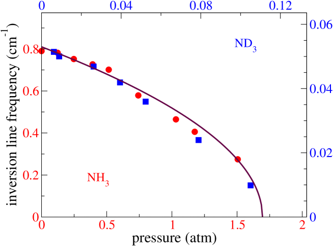
Figure 1: Measured inversion-line frequency $\bar{\nu}$ as a function of the gas pressure $P$ for $NH_{3}$ (dots, left and bottom scales, data from BL) and $ND_{3}$ (squares, right and top scales, data from BM). The solid line is the theoretical formula (10) with $P_{\mathrm{cr}}=1.695$ atm for $NH_{3}$ and $P_{\mathrm{cr}}=0.111$ atm for $ND_{3}$ calculated according to (9).

At pressures greater than the critical one we have the following situation. In the limit of an infinite number of molecules, the Hilbert space separates into two sectors generated by the ground state vectors given in mean field approximation by

$$|\psi_{0}^{L}\rangle = |\lambda_{0}^{L}\rangle\ldots|\lambda_{0}^{L}\rangle$$ (12)

$$|\psi_{0}^{R}\rangle = |\lambda_{0}^{R}\rangle\ldots|\lambda_{0}^{R}\rangle\ .$$ (13)

These sectors, which we call $\cal{H}_{L}$ and $\cal{H}_{R}$, cannot be connected by any operator involving a finite number of degrees of freedom (local operator). This means that a superselection rule operates between them.

2.3 Chiral molecules as a case of SSB

The mean field model outlined in the previous subsection has the essential features of SSB however with some peculiar aspects. Our model describes, according e.g. to the definition of SS, a quantum phase transition involving only the inversion degree of freedom of the molecules. We have assumed in fact a separation of the inversion dynamics from the rotational and translational degrees of freedom. In this respect there may be a difference between a molecule of the form $XY_{3}$ and an optically active molecule $XYZW$ which is less symmetric and a coupling with rotational degrees of freedom is to be expected. However according to T, empirically the decoupling appears to work reasonably well also in this case. In view of the success of our model in reproducing the experimental results in spite of the simplification of the actual system, an effort must be made to derive it from the complete dynamics involving all the degrees of fredom of the molecules. Work is in progress on this problem. Furthermore, considering that the measurements were taken long ago, new experiments seem desirable.

A similar treatment can be applied to a gas of pyramidal molecules of very low density in an environment provided by a gas of higher density of molecules of a different kind. In this case one may neglect the interaction among the pyramidal molecules and reduce the problem to a single molecule interacting with the environment. If this is made of units having a dipole moment the situation is not substantially different from the one discussed above. If the molecules of the environment are not endowed with a dipole moment they can acquire it through deformation under the action of the field of the pyramidal molecules. This is again the reaction field mechanism. Of course the localizing effect is much weaker and, for example, in a gas of $He$ the critical pressure for $NH_{3}$ is of the order of $7.3\cdot 10^{3}\>atm$ which is still experimentally accessible in the laboratory.

In a recent work by Trost and Hornberger [13] the localization problem is analysed in detail from a dynamical point of view. The basic idea of the mechanism is that through repeated scatterings in a host gas producing decoherence, a molecule is blocked in a localized state. Dissipation is involved in the process. It is not easy to compare the dynamical approach with our theory. Let us consider the previous case of a pyramidal molecule in a non-chiral gas. From our point of view the localized state of the molecule, while not an eigenstate of the isolated molecule, corresponds to a stationary state of the system formed by the molecule and the gas. Other situations where this point of view turns out to be useful were discussed in JLC. If I understand correctly the dynamical point of view, the molecule remains in a non stationary state for ever due the environment but the stationary states of the composite system are never considered. In MS Simonius claimed that the dynamical blocking of states “differs from, and is much more powerful than, the one [SSB] usually discussed in the literature based on nonsymmetric solutions to symmetric equations”. In my opinion, there is not yet a satisfactory understanding of when the decoherence picture applies. For example in conditions of temperature and pressure in which the inversion line due to tunneling is observed the dynamical mechanism must be ineffective. However one can conceive situations in which the two pictures are complementary descriptions of the same reality.

We emphasize that so far the SSB interpretation of molecular chirality, besides being conceptually simple, provides for the first time a theory having a qualitative and quantitative support from the empirical data. These matters will be discussed in detail in a forthcoming paper JLP. For a general assessment of the problem of chiral molecules see also ASW.

3 Magnetic pairing

The presence of a magnetic field can generate new interesting phenomena in three-dimensional gauge theories as was recognized long ago by Hosotani [25]. At about the same time Gusynin, Miransky and Shovkovy discussed chiral symmetry breaking in NJL models with magnetic field as mentioned before. The phenomenon of chiral symmetry breaking in presence of an external homogeneous magnetic field of an internal $U(2)$ symmetry for the Dirac field in $2+1$ dimensions has recently attracted new attention. The reason why people are interested in this phenomenon is its possible relevance in the physics of two-dimensional systems like graphene, see e.g. KY,RMP and references therein.

In the following we discuss the construction of the Hilbert space for a Dirac field in $2+1$ dimensions under the action of an external magnetic field for any value of the mass. This is done in two steps which exhibit two levels of pairing. There is a first level in which pairs of operators of opposite momentum in the fourier development of the free field appear, giving rise to a new Fock space. In this space we introduce creation and destruction operators associated to the wave functions characterizing the Landau states which depend on a discrete index $n$. A subsequent pairing of such operators leads to a second Fock space which is the Hilbert space of the full relativistic problem. It is a rather peculiar structure which, as far as I know, was not encountered before.

3.1 Preliminaries

In the following we use units with $\hbar=c=1$ where $c$ is the velocity of light, as their values do not play a role in our discussion. Consider the Lagrangian $\mathcal{L}$:

$$\begin{split}{\mathcal{L}}&={\bar{\psi}}^{B}(x)\left[i\gamma^{\mu}{\mathcal{D}}_{\mu}-m\right]\psi^{B}(x)\\ {\mathcal{D}}_{\mu}&=\partial_{\mu}-ieA_{\mu}\;,\end{split}$$ (14)

where ${\bar{\psi}}^{B}(x)$ is the Dirac quantized field in presence of the vector potential $A_{\mu}$ and $e$ is the modulus of the electron charge. Since the magnetic field is constant and homogeneous we can choose the Landau gauge:

$$A_{\mu}=-\delta_{\mu 1}Bx_{2}\ .$$ (15)

Notice that introducing the magnetic length $l=1/(eB)^{1/2}$ and using it as a unit for the space time variables, the magnetic field can be rescaled to the value $1$. However in the following we shall keep the magnetic field explicit.

The problem of a free Dirac field, minimally coupled to a homogeneous magnetic field, can be exactly solved and in the Landau gauge the expression of the Dirac field in the so called chiral version [4, 7] is ($eB>0$):

$$\psi^{B}(x)=\begin{pmatrix}\psi_{1}^{B}(x)\\ \psi_{2}^{B}(x)\end{pmatrix}$$ (16)

$$\psi_{1}^{B}(x)=\sum_{n=0}^{\infty}\sum_{p_{1}}\{u_{np_{1}}(x)a_{np_{1}}+v_{n-p_{1}}(x)b_{np_{1}}^{\dagger}\}$$ (17)

$$\psi_{2}^{B}(x)=\sum_{n=0}^{\infty}\sum_{p_{1}}\{u_{np_{1}}^{(2)}(x)c_{np_{1}}+v_{n-p_{1}}^{(2)}(x)d_{np_{1}}^{\dagger}\}$$ (18)

$$\begin{split}u_{np_{1}}(x)&=\frac{1}{\sqrt{lL_{1}}}e^{-iE_{n}t}e^{ip_{1}x_{1}}\begin{pmatrix}A_{n}w_{n}(\xi_{x_{2}}^{p_{1}})\\ -iB_{n}w_{n-1}(\xi_{x_{2}}^{p_{1}})\end{pmatrix}\\ v_{np_{1}}(x)&=\frac{1}{\sqrt{lL_{1}}}e^{+iE_{n}t}e^{ip_{1}x_{1}}\begin{pmatrix}B_{n}w_{n}(\xi_{x_{2}}^{p_{1}})\\ +iA_{n}w_{n-1}(\xi_{x_{2}}^{p_{1}})\end{pmatrix}\end{split}$$ (19)

$$u_{np_{1}}^{(2)}(x)=(-1)^{n}v_{n-p_{1}}(-x)\quad v_{np_{1}}^{(2)}(x)=(-1)^{n}u_{n-p_{1}}(-x)$$ (20)

$$A_{n}=\sqrt{\frac{E_{n}+m}{2E_{n}}}\qquad B_{n}=\sqrt{\frac{E_{n}-m}{2E_{n}}}$$ (21)

$$E_{n}=\sqrt{m^{2}+2neB}\qquad\xi_{x_{2}}^{p_{1}}=\frac{x_{2}}{l}+lp_{1}=\sqrt{eB}x_{2}+\frac{p_{1}}{\sqrt{eB}}$$ (22)

$$w_{n}(\xi)=c_{n}e^{-\xi_{2}/2}H_{n}(\xi)=\left(2^{n}n!\sqrt{\pi}\right)^{-1/2}e^{-\xi^{2}/2}H_{n}(\xi)\ .$$ (23)

The operators $a_{np_{1}},...,d_{np_{1}}$ satisfy canonical anticommutation relations and $H_{n}(\xi)$ are the Hermite polynomials. The case $eB<0$ can be obtained by applying the charge conjugation operator. For a discussion of the symmetry properties of the problem we refer to JLM,GMS. Here we only mention that apart from the mass term the Lagrangian is invariant under chiral transformations and in the limit $m\rightarrow 0$ in $2+1$ dimensions there is spontaneous symmetry breaking revealed by the calculation of the order parameter

$$\lim_{m\to 0}\langle B|\bar{\psi}^{B}(x)\psi^{B}(x)|B\rangle=-{\frac{|eB|}{2\pi}}.$$ (24)

The problem solved in JLM was the calculation of the formal relationship between the Dirac field in presence of magnetic field and the free Dirac field,

$$\psi_{1}(x)=\sum_{\bm{p}}\sqrt{\frac{m}{L_{1}L_{2}E_{\bm{p}}}}\left\{u(\bm{p})e^{-ip\cdot x}a_{\bm{p}}+v(\bm{p})e^{ip\cdot x}b_{\bm{p}}^{\dagger}\right\}$$ (25)

$$u(\bm{p})=\sqrt{\frac{E_{\bm{p}}+m}{2m}}\begin{pmatrix}1\\ \frac{p_{2}-ip_{1}}{E_{\bm{p}}+m}\end{pmatrix}\quad v(\bm{p})=\sqrt{\frac{E_{\bm{p}}+m}{2m}}\begin{pmatrix}\frac{p_{2}+ip_{1}}{E_{\bm{p}}+m}\\ 1\end{pmatrix}\;,$$ (26)

where $E_{\bm{p}}=(m^{2}+|\bm{p}|^{2})^{1/2}$. Similarly for $\psi_{2}$.

Following NJL we obtained the desired relationship by imposing the same initial condition on the Dirac equations describing the free field and the one in presence of the external magnetic field,

$$\psi_{i}(0,{x})=\psi_{i}^{B}(0,{x})\quad i=1,2\ .$$ (27)

3.2 Constructing the Hilbert space

The following presentation reverses to some extent the order of the calculation in JLM but this helps in bringing out the main points. From JLM it is clear that there is a natural ambient space for the construction of the vacuum of the Dirac field in $2+1$ dimensions with constant magnetic field. Let us define

$$A_{p}=\sqrt{\frac{E_{p}+m}{2Ep}}(a_{p}-C_{p}b^{{\dagger}}_{-p})$$ (28)

$$B_{p}=\sqrt{\frac{E_{p}+m}{2Ep}}(C_{p}a^{{\dagger}}_{p}+b_{-p})\;,$$ (29)

with

$$C_{\bm{p}}=\frac{p_{2}+ip_{1}}{E_{\bm{p}}+m}\qquad.$$ (30)

The operators $A_{p},A^{\dagger}_{p}$ and $B_{p},B^{\dagger}_{p}$ satisfy the usual canonical anticommutation relations (CAR). The corresponding vacuum is

$$|\hat{0}\rangle=\prod_{\bm{h}}\frac{E_{\bm{h}}+m}{2E_{\bm{h}}}\left(1+C_{\bm{h}}a_{\bm{h}}^{\dagger}b_{-\bm{h}}^{\dagger}\right)|0\rangle\ .$$ (31)

By applying the operators $A_{p}^{\dagger},B_{p}^{\dagger}$ to $|\hat{0}\rangle$ we generate a new Fock space where a first pairing appears. Notice that pairs carry a phase which depends on the momentum.

We next introduce the creation and destruction operators

$$\begin{split}\widehat{a}_{np_{1}}=A(f_{np_{1}})&=\sum_{p_{2}}f_{np_{1}}(p_{2})A_{p}\\ \widehat{b}_{n-p_{1}}=B(-if_{n-1\;-p_{1}})&=\sum_{p_{2}}-if_{n-1\;-p_{1}}(p_{2})B_{p}\;,\end{split}$$ (32)

where

$$f_{np_{1}}(p_{2})=i^{n}\sqrt{2\pi l}e^{-il^{2}p_{1}p_{2}}w_{n}(lp_{2})\;,$$ (33)

are the fourier transform in one variable of the wave functions appearing in (19).

The main result of JLM is the identification of the operators $a_{np_{1}},b_{np_{1}}$ appearing in (17) with those defined by the Bogolyubov transformation

$$\left\{\begin{aligned} a_{np_{1}}&=A_{n}\widehat{a}_{np_{1}}-B_{n}\widehat{b}_{n-p_{1}}^{\dagger}\\ b_{n-p_{1}}&=A_{n}\widehat{b}_{n-p_{1}}+B_{n}\widehat{a}_{np_{1}}^{\dagger}\ .\end{aligned}\right.$$ (34)

A similar analysis can be done for $\psi_{2}^{B}$ introducing operators $\widehat{c}_{np_{1}}$ and $\widehat{d}_{np_{1}}$ and using the equations (18), (20).

The previous discussion then leads to the following expression for the vacuum of the Dirac field in presence of a constant magnetic field

$$|B\rangle=\prod_{n\geq 1}\prod_{p_{1}}\left(A_{n}+B_{n}{\widehat{a}_{np_{1}}}^{\dagger}{\widehat{b}_{n-p_{1}}}^{\dagger}\right)\left(A_{n}-B_{n}{\widehat{c}_{np_{1}}}^{\dagger}{\widehat{d}_{n-p_{1}}}^{\dagger}\right)|\hat{0}\rangle\;,$$ (35)

where,

$$|\hat{0}\rangle=\prod_{\bm{h}}\frac{E_{\bm{h}}+m}{2E_{\bm{h}}}\left(1+C_{\bm{h}}a_{\bm{h}}^{\dagger}b_{-\bm{h}}^{\dagger}\right)\left(1+C_{\bm{h}}^{\ast}c_{\bm{h}}^{\dagger}d_{-\bm{h}}^{\dagger}\right)|0\rangle\ .$$ (36)

We emphasize once more that this expression holds for any value of $m$. By applying the conjugate of the operators defined in (34), and the corresponding ones associated to $\psi_{2}$, to the vacuum $|B\rangle$ we generate the full Hilbert space of the Dirac field in a magnetic field.

A simple calculation shows that $\langle 0|\hat{0}\rangle=0$ and $\langle\hat{0}|B\rangle=0$. Therefore three Fock spaces orthogonal to each other are involved in the diagonalization of the Hamiltonian of a Dirac field in presence of a constant magnetic field in $2+1$ dimensions.

In order to clarify the meaning of the hatted operators, following JLM, let us write the Hamiltonian in presence of magnetic field in terms of these operators. Using (34) we find

$$\begin{split}\displaystyle\mathrm{H}^{B}&=\widehat{\mathrm{H}}-\sum_{n=1}^{\infty}\sum_{p_{1}}\sqrt{2neB}\left({\widehat{a}_{np_{1}}}^{\dagger}{\widehat{b}_{n-p_{1}}}^{\dagger}+\widehat{b}_{n-p_{1}}\widehat{a}_{np_{1}}\right)\\ \displaystyle\widehat{\mathrm{H}}&\equiv m\sum_{n=0}^{\infty}\sum_{p_{1}}\left({\widehat{a}_{np_{1}}}^{\dagger}\widehat{a}_{np_{1}}+{\widehat{b}_{np_{1}}}^{\dagger}\widehat{b}_{np_{1}}\right)\ .\end{split}$$ (37)

The expression of the Hamiltonian $\widehat{\mathrm{H}}$ shows that $\widehat{a}_{np_{1}}$ and $\widehat{b}_{np_{1}}$ describe particles with degenerate energy $m$, that is the energy of the lowest Landau level (LLL). The magnetic field induces creation and destruction of particle-antiparticle pairs of the auxiliary field and this removes the degeneracy giving the usual Landau levels. It is easy to see that $\widehat{H}$ does not depend on the magnetic field $B$. Using the completeness of Hermite functions it can be rewritten as $m\sum_{p}(A^{\dagger}_{p}A_{p}+B^{\dagger}_{p}B_{p})$. A decomposition similar to (37) holds for the free Hamiltonian of the massive field in NJL models without magnetic field: the creation and destruction operators of the massless field play the role of the hatted operators and the mass replaces the magnetic field in the quadratic interaction.

3.3 Magnetic pairing and magnetic catalysis

Let us summarize what emerges from the previous analysis. A characteristic feature of SSB with a mechanism akin to supeconductivity is a pairing of particles and antiparticles. This is what happens in the NJL model [6] where the pairing is due to the attractive nonlinear interaction provided it is sufficiently strong. In the previous subsection we have shown that pairing is induced in a free Dirac field in $2+1$ dimensions by a constant magnetic field for any value of the mass. There is no surprise therefore that when we switch on the nonlinear interaction in the limit of zero mass chiral SSB takes place even for very small values of the coupling. In $2+1$ dimensions the dependence of the dynamical mass on the nonlinear coupling is analytic as shown in [4]. The point of view discussed in this paper complements the analysis of Gusynin, Miransky and Shovkovy. The magnetic catalysis appears as a special consequence of the more general phenomenon represented by magnetic pairing.

4 Spontaneous symmetry breaking in nonequilibrium

SSB has been studied so far mainly as an equilibrium phenomenon typical of systems with infinitely many degrees of freedom. It was discovered however some time ago [8] that out of equilibrium SSB can take place through mechanisms not available in equilibrium. For example, it is well known that in one-dimensional systems with short range interactions like a one-dimensional Ising model, SSB is not possible. However it was shown that in one-dimensional models through which currents are flowing due to unequal boundary conditions at the two sides of the system, stationary states breaking a symmetry are possible. In the cases considered the broken symmetry is $CP$, the product of charge conjugation and parity. In spite of the fact that fifteen years have elapsed the study of these models is still at the beginning and there are very few rigorous results. This may be due to the great difficulties encountered in non equilibrium physics or also to the lack of other major motivations. One motivation of the models apparently was provided by traffic problems, therefore not connected with condensed matter or particle physics. They are very special but I wish to emphasize the important message they convey:

Stationary states are the obvious generalization of equilibrium states but the conditions under which SSB takes place in nonequilibrium are different from equilibrium. In stationary nonequilibrium states SSB may be possible even when it is not permitted in equilibrium.

We describe briefly the class of one-dimensional models introduced in PEM which belongs to the category of boundary driven particle systems. One considers a one dimensional lattice of length $N$, called the bridge, where each point can be occupied either by a positive $(+)$ or a negative $(-)$ particle or be empty $(0)$. The positive particles move to the right while the negative particles move to the left with hard core exclusion. At each end of the bridge there are junctions where the lattice splits into two parallel segments, access and exit lanes, one containing only plus particles and empty sites and the other only minus particles and empty sites.

Plus particles are injected in the access lane at the left with rate $\alpha$, if the first site is empty, and removed with rate $\beta$ from the right end of the exit lane (on the right of the lattice), if the last site is occupied. Likewise minus particles are injected into their access lane on the right with rate $\alpha$ and removed with rate $\beta$ from the left end of their exit lane. Plus and minus particles hop with rate $1$ to the right and to the left, respectively, in their access-exit lanes. Plus particles enter the bridge at the left junction if the first site is empty and leave it at the other junction if the first site of the exit lane is empty, with rate $1$. Inside the bridge plus particles exchange with empty sites and with minus particles with rate $1$. The same rules hold for the minus particles after exchanging right with left. The model is clearly symmetric with respect to simultaneous charge conjugation and left-right reflection.

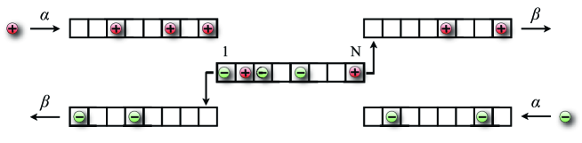
Figure 2: The bridge model with access and exit lanes after PEM

Summarizing the dynamics, during a time interval $dt$ three types of exchange events can take place between two adjacent sites

$$+0\rightarrow 0+\;,\quad 0-\rightarrow-0\;,\quad+-\rightarrow-+\;,$$ (38)

with probability $dt$. The last one takes place only on the bridge. At the left of the access lane of plus particles we have

$$0\rightarrow+\;,$$ (39)

with probability $\alpha dt$. At the right end of the exit lane of plus particles

$$+\rightarrow 0\;,$$ (40)

with probability $\beta dt$, and similarly for minus particles after reflection. One is interested in the steady states in the thermodynamical limit $N\rightarrow\infty$. These are characterized by the density profiles of the two charges and the corresponding currents.

The phase diagram of this system in the $(\alpha,\beta)$ plane exhibits three phases of which two are symmetric, i.e. the densities and currents of the two charges are the same, and one is non symmetric. The symmetry breaking phase exists for low values of the rate $\beta$. In this phase the densities and currents of the positive and negative particles are different. There are two stationary states breaking the $CP$ symmetry in which either the positive particles or the negative particles dominate.These states are obtained one from the other by applying the $CP$ operation. For finite $N$ jumps between these states are possible but one can prove that the mean jump time diverges exponentially with $N$ so that they become stable in the thermodynamic limit. For details the reader is referred to PEM.

4.1 Possible relevance of nonequilibrium SSB

There are facts in the world around us that so far have eluded a really satisfactory explanation. At the planetary scale we know that in living matter left-handed chiral molecules are the rule. The question was raised by Pasteur in the XIXth century [28]. Explanations have been attempted for example invoking a small initial unbalance between left-handed and right-handed molecules in the prebiotic world subsequently amplified through various mechanisms [29]. The effects of parity violation in weak interations also have been considered [30]. I think that nonequilibrium SSB in stationary states offers another direction to be explored. Kinetic models based on nonequilibrium stationary states, therefore closer to the point of view advocated here, have been proposed, see e.g. PBC. What is missing however is a full statistical mechanics approach to the problem allowing to disentangle the general mechanism from the chemical details of each model.

At the cosmic scale we do not understand completely why matter is so much more abundant than antimatter. Also in this case explanations have been proposed based on evolutionary nonequilibrium invoking small symmetry violations which are amplified to reach the present state of the universe. For recent reviews see YO,SH. These explanations, in which nonequilibrium is a fundamental ingredient, require a detailed reconstruction of the histories which are complicated and with many uncertainties. What I am suggesting here is another way in which nonequilibrium may play a role. Stationary or quasi-stationary nonequilibrium states in which symmetries are spontaneously broken may appear during an evolutionary process. The dynamics of currents is the additional ingredient which enriches the picture with respect to equilibrium. This may require some departure from the prevailing picture of the early history of our universe.

Nonequilibrium stationary states with SSB deserve further study both as a purely theoretical problem and in view of applications to natural phenomena. A first step is to study this phenomenon in dimension greater than one. We point out that generically new types of phase transitions arise in nonequilibrium. They are connected with singularities of the free energy not permitted in equilibrium [34]. Moreover the thermodynamics of current fluctuations shows that dynamical phase transitions spontaneously breaking translation invariance in time, are possible [35, 36]. One should profit of this wider perspective in the study of old and new problems.

References

- [1] F. Hund, Z. Phys. 43 (1927), 805.
- [2] P. Claverie, G. Jona-Lasinio, Phys. Rev. A 33 (1986), 2245.
- [3] G. Jona-Lasinio, C. Presilla, C. Toninelli, Phys. Rev. Lett. 88 (2002), 123001.
- [4] V. P. Gusynin, V. A. Miransky, I. A. Shovkovy, Phys. Rev. D 52 (1995), 4718.
- [5] V. P. Gusynin, V. A. Miransky, I. A. Shovkovy, Nucl.Phys. B 462 (1996), 249.
- [6] Y. Nambu, G. Jona-Lasinio, Phys. Rev, 122 (1961), 345.
- [7] G. Jona-Lasinio, F. M. Marchetti, Phys. Lett. B 459 (1999), 208.
- [8] M. R. Evans, D. P. Foster, C. Godrèche, D. Mukamel, Phys. Rev. Lett. 74 (1995), 208.
- [9] V. Popkov, M. R. Evans, D. Mukamel, J. Phys. A: Math. Theor. 41 (2008), 432002.
- [10] S. Gupta, D. Mukamel, G. M. Schütz, J. Phys. A: Math. Theor. 42 (2009), 485002.
- [11] M. Simonius, Phys.Rev. Lett. 40 (1978), 980.
- [12] R. A. Harris, L. Stodolsky, J. Chem. Phys. 74 (1981), 2145.
- [13] J. Trost, K. Hornberger, Phys. Rev. Lett. 103 (2009), 023202.
- [14] G. Jona-Lasinio, F. Martinelli, E. Scoppola, Comm. Math. Phys. 80 (1981), 223.
- [15] G. Jona-Lasinio, F. Martinelli, E. Scoppola, Phys. Rep. 77 (1981), 313.
- [16] Bleaney, J. H. Loubster, Nature 161, 522 (1948), Proc. Phys. Soc. London Sec. A 63,483 (1950)
- [17] G. Birnbaum, A. Maryott, Phys. Rev. 92, 270 (1953)
- [18] G. Gallavotti, Rivista del Nuovo Cimento 2 (1972), 133.
- [19] R. E. Weston Jr., J. Am. Chem. Soc. 76 (1954), 2645.
- [20] C. H. Townes, A. L. Schawlow, Microwave Spectroscopy (MacGraw-Hill, N.Y. 1955).
- [21] S. Sachdev, Quantum Phase Transitions, Cambridge University Press (1999).
- [22] G. Jona-Lasinio, P. Claverie, Prog. Theor. Phys. Supplement 86 (1986), 54.
- [23] G. Jona-Lasinio, C. Presilla, paper in preparation.
- [24] A. S. Wightman, Some comments on the quantum theory of measurement, in Probability methods in mathematical physics, F. Guerra, M. I. Loffredo, C. Marchioro eds. (World Scientific, Singapore) 1992, p. 411 and Nuovo Cimento 110B (1995), 751.
- [25] Y. Hosotani, Phys. Rev. D 51 (1995), 2022.
- [26] Kun Yang, Solid State Comm. 143 (2007), 27.
- [27] A. H. Castro et al., Rev. Mod. Phys. 81 (2009),109.
- [28] L. Pasteur, Oeuvres complètes, Tome I, (1922), 369.
- [29] D. G. Blackmond, Cold Spring Harb. Perspect. Biol. (2010);2:a002147.
- [30] A. Salam, J. Mol. Evol. 33 (1991), 105.
- [31] R. Plasson, H. Bersini, A. Commeyras, PNAS 101 (2004), 16733.
- [32] M. Yoshimura, J. Phys. Soc. Japan 76 (2007), 111018.
- [33] M. Shaposhnikov, Journal of Physics: Conference Series 171 (2009), 012005.
- [34] L. Bertini, A. De Sole, D. Gabrielli, G. Jona-Lasinio, C. Landim, Lagrangian phase transitions in nonequilibrium thermodynamic systems, arXiv:1005.1489 .
- [35] L. Bertini, A. De Sole, D. Gabrielli, G. Jona-Lasinio, C. Landim, Phys. Rev. Lett. 94 (2005), 030601; J. Stat. Phys. 123 (2006), 237.
- [36] T. Bodineau, B. Derrida, Phys. Rev. E 72 (2005), 066110.