The Interplay of Magnetic Fields, Fragmentation and Ionization Feedback in High-Mass Star Formation

Abstract

Massive stars disproportionately influence their surroundings. How they form has only started to become clear recently through radiation gas dynamical simulations. However, until now, no simulation has simultaneously included both magnetic fields and ionizing radiation. Here we present the results from the first radiation-magnetohydrodynamical (RMHD) simulation including ionization feedback, comparing an RMHD model of a 1000 $M_{\odot}$ rotating cloud to earlier radiation gas dynamical models with the same initial density and velocity distributions. We find that despite starting with a strongly supercritical mass to flux ratio, the magnetic field has three effects. First, the field offers locally support against gravitational collapse in the accretion flow, substantially reducing the amount of secondary fragmentation in comparison to the gas dynamical case. Second, the field drains angular momentum from the collapsing gas, further increasing the amount of material available for accretion by the central, massive, protostar, and thus increasing its final mass by about 50% from the purely gas dynamical case. Third, the field is wound up by the rotation of the flow, driving a tower flow. However, this flow never achieves the strength seen in low-mass star formation simulations for two reasons: gravitational fragmentation disrupts the circular flow in the central regions where the protostars form, and the expanding H ii regions tend to further disrupt the field geometry. Therefore, ionizing radiation is likely to dominate outflow dynamics in regions of massive star formation.

1. Introduction

Massive stars influence their surroundings through their ionizing radiation, winds, and supernova explosions. However, their formation remains less well understood than that of low mass stars (Mac Low & Klessen 2004). Massive stars accrete much faster than low mass stars at rates reaching as high as $10^{-3}M_{\odot}\mathrm{yr}^{-1}$ (e.g. Beuther et al. 2002). This is required to build up the mass of the star prior to exhausting its nuclear fuel (Keto & Wood 2006). They are observed to have companions with far greater frequency than low mass stars (Lada 2006; Zinnecker & Yorke 2007). The ionizing radiation they emit produces a set of observables distinctly different from low mass star formation.

Magnetic fields pervade neutral atomic gas in the interstellar medium at strengths high enough to prevent isotropic gravitational collapse (Heiles 1976). However, gravitational collapse along field lines can proceed unimpeded, and, in some circumstances, magnetic fields can even accelerate collapse through magnetic braking (Kim et al. 2003; Hennebelle & Ciardi 2009). Observations of low-mass star forming regions show that magnetic field strength remains roughly constant at values of $B=$ 5–10 $\mu$G at number densities $n<10^{3}\,$cm^-3, with the strength growing as $B\propto n^{2/3}$ at higher number densities (Crutcher 2009).

The role of magnetic fields in low mass star formation has received extensive attention. They act in three major ways. First, they can provide support against gravitational collapse. Second, they drain angular momentum directly through magnetic braking, as well as indirectly through magnetorotational instability driven turbulent viscosity. Finally, as one consequence of angular momentum transport, they drive jets and outflows.

The critical mass-to-flux ratio at which magnetic fields can no longer support a gas cloud against gravitational collapse is (Mouschovias & Spitzer 1976; Mouschovias 1991)

$$\left(\frac{M}{\Phi}\right)_{\mathrm{cr}}=\frac{\zeta}{3\pi}\left(\frac{5}{G}\right)^{1/2}=490\mbox{ g G}^{-1}\mathrm{cm}^{-2}$$ (1)

where $\zeta=0.53$ is the value for a uniform sphere (Strittmatter 1966). For a field of 10 $\mu$G, this corresponds to a column density of $5\times 10^{-2}$ g cm^-2, well below the 0.1-1 g cm^-2 characteristic of massive star forming regions (e.g. Mueller et al. 2002; McKee & Tan 2003; Krumholz & McKee 2008). As a result, less attention has been paid to the dynamics of magnetic fields in massive star forming regions where it appeared unlikely that they would prevent star formation (see, however, Hennebelle et al. 2010, A& A submitted).

However, even in models of low-mass star formation starting with supercritical values of $(M/\Phi)$, fragmentation is reduced compared to the pure gas dynamical case by a combination of magnetic pressure and tension forces providing additional support to counteract gravitational collapse (Ziegler 2005; Banerjee & Pudritz 2006; Price & Bate 2007; Hennebelle & Fromang 2008; Hennebelle & Teyssier 2008; Hennebelle & Ciardi 2009; Commerçon et al. 2010; Bürzle et al. 2010).

Magnetic fields can also drain angular momentum from rotating clumps and cores even if they do not entirely prevent collapse. Magnetic braking in idealized perpendicular and parallel cases was computed by Mouschovias & Paleologou (1979, 1980), who found the criterion for braking to be effective is that outgoing helical Alfvén waves pass through a mass of external gas equal to that of the cloud (see also Basu & Mouschovias 1994; Hennebelle & Ciardi 2009).

Magnetorotational instability further drives outward angular momentum transport within differentially rotating disks, or indeed any differentially rotating structure with angular velocity decreasing outward (Balbus & Hawley 1991, 1998). This may be less important in massive star forming regions where gravitational instability dominates angular momentum transport (Peters et al. 2010a, b).

Outflows have been found almost universally around forming low mass stars. Controversy persists about the exact mechanism driving them (Ferreira et al. 2006), with viable suggestions including disk winds (Blandford & Payne 1982; Königl & Pudritz 2000), tower flows produced by wound up toroidal field (Tomisaka 1998, 2002; Matsumoto & Tomisaka 2004; Machida et al. 2004; Banerjee & Pudritz 2006, 2007) or interactions between the disk field and protostellar magnetosphere, either at an X-point (Najita & Shu 1994; Shu et al. 1994, 2007; Cai et al. 2008) or in more general geometries (Lovelace et al. 1999; Romanova et al. 2009). However, all these mechanisms depend on the interaction of magnetic fields with a coherent and well-defined rotational flow in the accretion disk.

In this work we use numerical simulations to examine more carefully the dynamics of magnetic fields during the formation of massive stars, focussing on the clump scale of 0.1 to 0.001 pc. We model the collapse of a magnetized, rotating clump containing 1000 $M_{\odot}$. This work is complementary to the initial numerical study of magnetic fields in massive star forming regions by Banerjee & Pudritz (2007) in that it examines a larger mass region at larger scales. It is also complementary to recent radiation-magnetohydrodynamical simulations of low-mass star formation by Tomida et al. (2010) because we take the feedback by ionizing and non-ionizing radiation into account. We show that the three ways that magnetic fields act in low mass star formation recur in massive star formation, but with different implications and relative importance.

In Section 2 we describe our numerical simulations, while in Section 3 we discuss our results. Finally, we summarize and conclude in Section 4.

2. Numerical Method and Initial Conditions

We present the first three-dimensional, radiation-magnetohydrodynamical simulations of massive star formation, taking into account heating by both ionizing and non-ionizing radiation, using the adaptive-mesh code FLASH (Fryxell et al. 2000). We propagate the radiation on the adaptive mesh with our extended version of the hybrid characteristics raytracing method (Rijkhorst et al. 2006; Peters et al. 2010a). We use sink particles (Federrath et al. 2010) to model young stars. Sink particles are inserted when the Jeans length of collapsing gas can no longer be resolved on the adaptive mesh. They continue to accrete any high-density gas lying within their accretion radius. We use the sink particle mass and accretion rate to determine the radiation feedback with a prestellar model (Peters et al. 2010a). The radiation-magnetohydrodynamical equations are solved with a novel, positive-definite, MUSCL-Hancock, Riemann solver (Waagan 2009).

In this work we present simulations that incorporate magnetic fields into the gas dynamical collapse models presented in Peters et al. (2010a). We further analyzed those models with a focus on the accretion history of the stellar cluster (Peters et al. 2010b), as well as the resulting H ii region morphologies (Peters et al. 2010c). The initial conditions for the gas and the simulation parameters in the simulations presented here match those in our previous simulations. We start with a $1000\,M_{\odot}$ molecular cloud having a constant density core with $\rho=1.27\times 10^{-20}\,$ g cm^-3 within a radius of $r=0.5\,$pc, surrounded by an $r^{-3/2}$ density fall-off out to $r=1.6\,$pc. The cloud rotates as a solid body with an angular velocity $\omega=1.5\times 10^{-14}\,$s^-1. The initial temperature is $T=30\,$K. The highest resolution cells on our adaptive mesh have a size of $98\,$AU. Sink particles are inserted at a cut-off density of $\rho_{\mathrm{crit}}=7\times 10^{-16}\,$g cm^-3 and have an accretion radius of $r_{\mathrm{sink}}=590\,$AU.

We compare the results of four different simulations (see Table 1), three of which were discussed and analyzed in our previous work (Peters et al. 2010a, c, b). In the first simulation (run A), a dynamical temperature floor is introduced to suppress secondary fragmentation. Only one sink particle (representing a massive protostar) is allowed to form. In the second simulation (run B), secondary fragmentation is allowed, and many sink particles form, representing a group of stars, each contributing to the radiative feedback. The third simulation (run D) is a control run in which secondary fragmentation is still allowed, but no radiation feedback is included.

The new, fourth simulation (run E) is a magnetized version of run B, the full stellar group simulation with radiation feedback from all stars. Run E includes an initially homogeneous magnetic field along the rotation axis of the cloud with a magnitude of $10\,\mu$G, corresponding to $(M/\Phi)=14(M/\Phi)_{\mathrm{cr}}$ in the central core at the beginning of the simulation and a plasma beta ($\beta_{\mathrm{pl}}=p_{\mathrm{th}}/p_{\mathrm{mag}}$ with the thermal and magnetic pressure $p_{\mathrm{th}}$ and $p_{\mathrm{mag}}$, respectively) of $\beta_{\mathrm{pl}}=3.7$ . This strength was chosen to be consistent with an analysis of combined H i , OH, and CN Zeeman measurements that yielded a field strength

$$B\simeq(10\,\mu\,\mathrm{G})\left(\frac{n}{300\mathrm{\,cm}^{-3}}\right)^{0.68}$$ (2)

(Crutcher et al. 2010, in prep; Crutcher 2010). Our choice of a uniform field initially neglects the increase of field strength with increasing density, but this occurs quickly as the collapse proceeds. We note that CN Zeeman observations by Falgarone et al. (2008) suggest a lower mass-to-flux ratio for high-density regions, as we would expect.

Table 1Overview of collapse simulations.

Name	Radiative Feedback	Multiple Sinks	Magnetic Fields
Run A	yes	no	no
Run B	yes	yes	no
Run D	no	yes	no
Run E	yes	yes	yes

3. Results and Discussion

3.1. Accretion History

The accretion history for run E is shown in Figure 1. The first sink particle that forms accretes more than $28\,M_{\odot}$ during the simulation runtime of $0.683\,$Myr, eventually becoming by far the most massive sink. Only after a delay of almost $20\,$kyr after the formation of the first sink do secondary sinks begin to form. None of them gets more massive than $6\,M_{\odot}$. In addition to the effect of radiation feedback, which raises the Jeans mass locally and reduces fragmentation (see Peters et al. 2010b for a thorough discussion), fragmentation is further reduced in this simulation by the magnetic field, just as is found in models of low-mass star formation (see Section 1). The same effects of reduced fragmentation occur even in our model of high-mass star formation with initial $(M/\Phi)\gg(M/\Phi)_{\mathrm{cr}}$.

Figure 1 also shows the accretion rates and protostellar masses of the first sinks to form in run A, run B, run D, and run E for comparison. The accretion rate in the initial accretion phase is higher in run E than in the other simulations, but the long-term accretion behavior does not appear to be substantially different, apart from a stronger variation beyond $0.64\,$Myr. However, we note that in run B, fragmentation-induced starvation (Peters et al. 2010a, b) terminates accretion onto a $23\,M_{\odot}$ sink, whereas the $28\,M_{\odot}$ sink in run E continues to accrete until the end of the simulation. The central star in run E can grow to larger masses because in the initial phase fragmentation is delayed by magnetic support. This allows the central object to maintain a high accretion rate for a longer time. Nevertheless, the accretion rate of the massive star in run E drops significantly when secondary sink particles form, since they form in a dense ring around the central massive sink and to some extent starve it of material, even though they never cut off accretion entirely.

The stronger initial accretion phase in run E compared to run B yields the main contribution to the larger final mass of the massive sink. The magnetic field very efficiently redistributes angular momentum, resulting in an increased radial mass flux through the high-density equatorial plane (see Section 3.2). Consequently, the initial accretion rate in the magnetized simulation (run E) even lies considerably above the non-magnetized single sink calculation (run A).

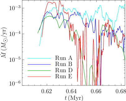
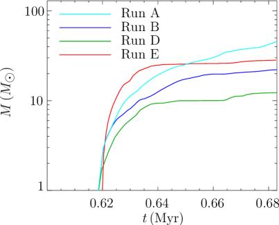
Figure 1.— (a) Accretion history for run E. The first sink that forms eventually becomes the only massive one to form during the simulation runtime. Radiative heating and magnetic support reduce fragmentation and lead to the formation of only a small number of sinks in comparison to the equivalent gas dynamical model. (b) Accretion rates of the first sink particles in run A, run B, run D and run E. While the initial accretion phase for the first sink in run E leads to a higher accretion rate, the long-term evolution of the accretion rates looks very similar. In contrast to run B, however, in which accretion onto the first star stopped when it had reached $23\,M_{\odot}$ after $0.70\,$Myr, accretion onto the $28\,M_{\odot}$ star in run E still continues (compare (c)). The accretion rate drops significantly when secondary sink particles form in run E. (c) Protostellar masses of the first sink particles in run A, run B, run D and run E. Radiative heating (run B) and presence of magnetic fields (run E) increase the final masses of the massive stars. The largest part of the additional mass accretion in run E compared to run B is due to the stronger initial accretion phase.

The total accretion histories of all sink particles combined in each of the four simulations are contrasted in Figure 2. For the first $20\,$kyr, the total accretion rate of run B, run D and run E is nearly identical. The accretion rate in these multiple sink simulations is generally higher than in the single sink run A since the large group of sinks accretes from a large volume, without needing to rely on outward angular momentum transport to deliver material to the direct feeding zone of the central sink. In the magnetized run E, no secondary sink particles form during the first $20\,$kyr (see Figure 1), so that the increased accretion rate in this phase is due to the additional angular momentum transport performed by the magnetic field. After the initial $20\,$kyr, the total accretion rate in run E falls below run B and the control run D, deviating increasingly with time, but always staying above the accretion rate in run A. The accretion histories of run B and run D only start to separate at relatively late time when the ionizing radiation begins to terminate accretion onto the most massive sinks in run B (see the discussion in Peters et al. 2010b), but the magnetic field additionally reduces the rate at which gas collapses in run E. Thus, the total accretion rate with magnetic fields is lower than without magnetic fields, in agreement with previous work by Wang et al. (2010) that used a stronger magnetic field.

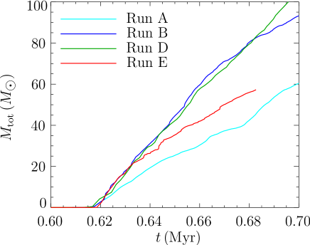
Figure 2.— Total accretion history of run A, run B, run D and run E. While the total accretion rates of run B and run D agree until ionization feedback stops massive star formation in run B, the total accretion rate in run E already starts to decline after $20\,$kyr. The magnetic field in run E additionally supports the gas against collapse, reducing the total accretion rate.

3.2. Magnetic Field Structure

As the molecular cloud collapses, it forms a thin, rotationally flattened structure in the midplane of the rotating cloud. This disk-like structure is very similar to the one we find in the run without magnetic fields. As this structure does not have a Keplerian rotation curve, we avoid calling it a disk, though it behaves in many ways similar to one. This structure is essentially what was called a pseudodisk by Galli & Shu (1993a, b). In the midplane, the dense, rotating gas drags the magnetic field with it, winding the magnetic field lines into a toroidal configuration that drives a magnetic tower flow (Uchida & Shibata 1985; Tomisaka 1998, 2002; Matsumoto & Tomisaka 2004; Machida et al. 2004; Banerjee & Pudritz 2006; Hennebelle & Fromang 2008). However, the magnetic tower can only build up as long as the field lines are anchored in a coherently rotating flow.

This velocity coherence is present initially but gets increasingly disrupted by fragmentation. Figure 3 shows slices of density, azimuthal velocity and vertical momentum through the midplane at three different times in run E. Initially, the whole region is rotating in the counterclockwise direction. As fragmentation proceeds, regions with clockwise (negative) azimuthal velocity appear near the center of collapse, and these regions expand radially with time. This means that the magnetic field lines that are anchored in the center cannot wind up anymore, and thus the vertical expansion of the magnetic tower flow stalls. The plots of vertical momentum of the gas show that the magnetic outflow is thereafter mostly launched from a ring around the center whose radius grows with time. The central regions, where the gas is rotating clockwise in some regions, eject little further material into the outflow.

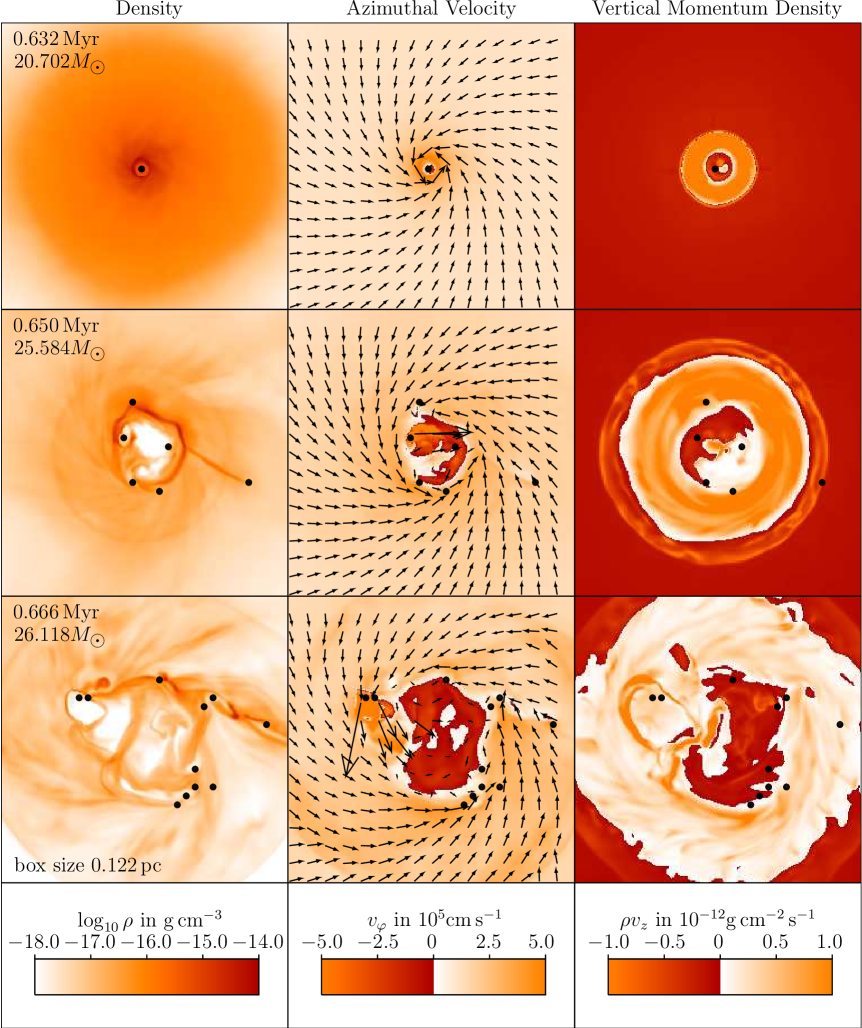
Figure 3.— Slices of gas density $\rho$, (left) and azimuthal velocity $v_{\varphi}$ (middle) in the midplane and (signed) vertical momentum density $\rho v_{z}$ (right) slightly above the midplane for three different snapshots of run E. The mass of the most massive star in the cluster is given in the images. Fragmentation sets in after the formation of the first filaments and sink particles (black dots). The resulting torques can reverse the direction of the azimuthal velocity component. The arrows indicate the direction of velocity. Although the cloud is initially rotating counterclockwise (white), the central region soon begins to rotate clockwise (red), and this region of reversed azimuthal velocity gradually expands. This has consequences for the driving of the magnetic outflow, visible in the slices of vertical momentum density (right). The outflow is primarily launched from its outer boundary, where coherent rotation is maintained, while momentum transport from the inner region is relatively weak. The online material contains an animated version of this figure.

Figure 4 illustrates why gravitational fragmentation poses a substantial problem to maintaining the magnetic tower flow. The figure shows density slices perpendicular to the midplane through the magnetic tower together with the magnetic field. Shortly after gravitational collapse has formed a dense structure in the midplane and sink particles have formed, the field lines are nicely aligned and anchored in the rotating, dense gas, so that a magnetic tower starts to build up. However, as gravitational fragmentation proceeds, the circular motion in the inner region gets increasingly disturbed by gravitational instability as well as angular momentum transport by the tower flow, resulting in a loss of velocity coherence. Hence, the magnetic tower grows laterally into regions where the velocity field remains coherent as fast as it grows in height, so it is unable to produce a collimated outflow. This structure is a magnetic bubble rather than the outflow we are familiar with in low-mass star formation (Cabrit & André 1991; Bachiller 1996; Reipurth & Bally 2001; Bally et al. 2007).

Although the velocity field is not turbulent initially, a substantial amount of turbulence develops during the simulation runtime because of gravitational fragmentation. Conversely, any initial turbulence will die away in a sound-crossing time (Mac Low et al. 1998). We do suspect that initialization with highly supersonic turbulence might modify the large-scale dynamics and the shape of filaments in our flattened structure but not that it will qualitatively change our results.

While it has been shown that magnetically driven outflows from low-mass stars can still form in a turbulent environment (Matsumoto & Hanawa 2010), it is less clear whether highly collimated, magnetically-driven outflows will persist around massive stars since turbulent fragmentation may even enhance the destructive effect of gravitational fragmentation discussed here on the velocity structure of disks around high-mass stars.

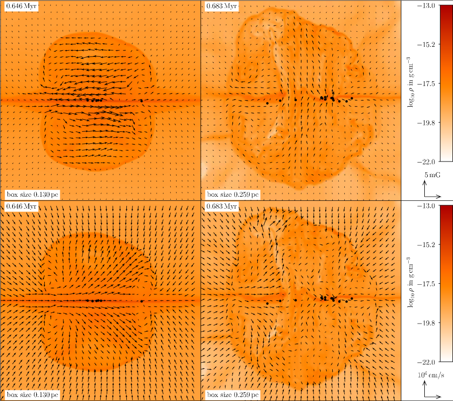
Figure 4.— Magnetic bubble and field structure. The images show density slices parallel to the rotation axis and perpendicular to the midplane through the magnetic bubble. The arrows indicate the direction of the magnetic field lines (top) and velocity (bottom), and the black dots show the positions of sink particles. In the initial phase (left), the field lines wind up to build up a magnetic tower flow. As the fragmentation occurs, the velocity coherence in the central regions disappears, so that magnetic field lines anchored there stop winding up (right). Hence, the magnetic bubble grows primarily laterally but does not form a more collimated outflow. Note the different spatial scales in the images.

H ii region formation further influences the magnetic field structure. Figure 5 shows slices of magnetic energy density and the plasma beta ($\beta_{\mathrm{pl}}=p_{\mathrm{th}}/p_{\mathrm{mag}}$ with the thermal and magnetic pressure $p_{\mathrm{th}}$ and $p_{\mathrm{mag}}$, respectively), along with magnetic field vectors. The left-hand plot demonstrates that the expansion of the H ii region driven by ionization heating reduces the magnetic energy content inside the H ii region of the most massive star in run E by more than four orders of magnitude. This is because the small amount of flux threading the initially ionized gas gets redistributed over the large volume that it expands into because of flux freezing. The alignment of the magnetic field, which remains visible outside the H ii region, also gets destroyed. The right-hand plot shows the same region after the former H ii region has completely recombined. The magnetic field energy has only increased slightly, since the gas has not been compressed much, and the magnetic field orientation is still disarranged.

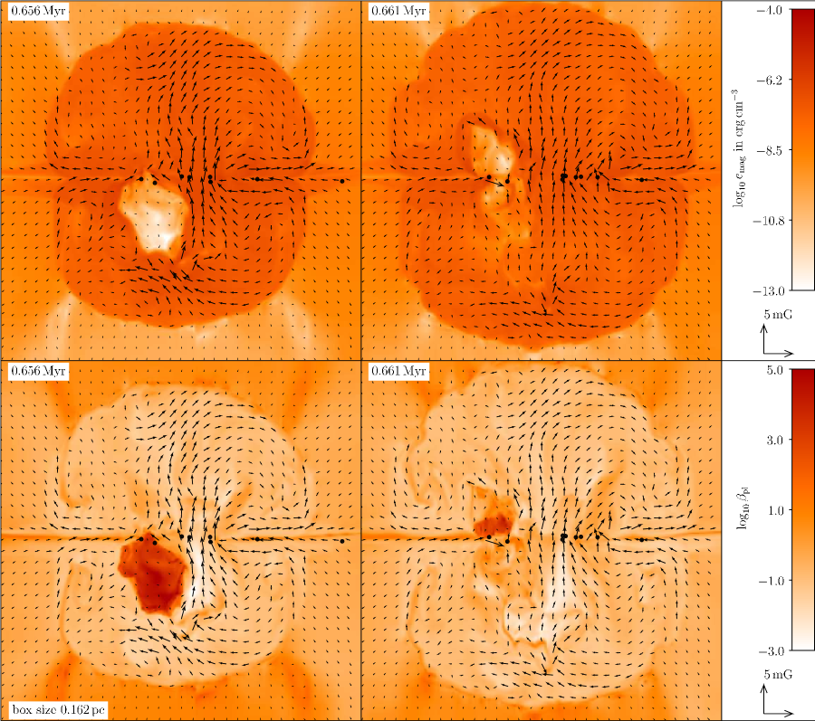
Figure 5.— Influence of ionizing radiation on magnetic field structure. The images show slices of magnetic energy density $e_{\mathrm{mag}}$ (top) and the plasma beta $\beta_{\mathrm{pl}}=p_{\mathrm{th}}/p_{\mathrm{mag}}$ (bottom) along with magnetic field vectors and sink particles. The ionizing radiation emitted by the most massive star of the cluster creates an H ii region, which dramatically decreases the magnetic energy content in this region and destroys the coherence of the magnetic field structure (left). After complete recombination of this H ii region, the magnetic energy density remains reduced and the magnetic field structure is not reconstructed (right). The black dots represent sink particles. The online material contains an animated version of this figure.

3.3. Gravitational and Magnetic Torques

To better understand the reasons for the breakdown of coherent rotation and the onset of counter-rotation in the flattened accretion flow, which ultimately disrupts the magnetic outflow, we study the different torques acting on the gas in the central regions. The torque $\tau$ exerted on the gas in the midplane (e.g., Banerjee & Pudritz 2006) is given by

$$\tau=r^{2}\int v_{r}\rho Rv_{\varphi}\,\mathrm{d}\Omega$$ (3)

with the spherical radius $r$, the radial velocity $v_{r}$, the cylindrical radius $R$, the azimuthal velocity $v_{\varphi}$ and the differential solid angle $\mathrm{d}\Omega$. Since the purely hydrodynamical simulation (run B) and the MHD calculation (run E) show fragmentation in the midplane, the negative torques required to reverse the direction of rotation should be present in both cases. Figure 6 demonstrates that his is indeed the case. The braking and reversal of the coherent velocity field is thus not a new phenomenon, but there are some notable differences in the fragmentation behavior.

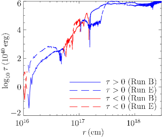
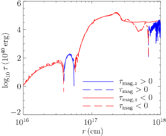
Figure 6.— (Left) The cumulative torque $\tau$ is plotted for the hydrodynamical simulation (run B) and for the MHD simulation (run E). Negative torques, indicating braking and reversal of the azimuthal velocity field, appear in both cases. (Right) Cumulative magnetic torques calculated in two different ways, the $z$-component of Equation (4) and via Equation (5). Deviations become visible only for radii $>10^{17}\,$cm, when the averaging volumes become disparate. The snapshot is taken from the end of run E, where the rotationally flattened flow is strongly fragmented and asymmetric.

While the only torques acting in the hydrodynamical case are gravitational, the magnetic field can exert additional torques

$$\bm{\tau}_{\mathrm{mag}}=\frac{1}{4\pi}\int\mathbf{r}\times\big{[}(\bm{\nabla}\times\mathbf{B})\times\mathbf{B}\big{]}\,\mathrm{d}V$$ (4)

on the gas in the MHD case. Under the assumption of cylindrical symmetry, the torque exerted by the magnetic field is

$$\tau_{\mathrm{mag}}=\frac{1}{4\pi}r^{2}\int B_{r}RB_{\varphi}\,\mathrm{d}\Omega$$ (5)

with the radial magnetic field component $B_{r}$ and the toroidal component $B_{\varphi}$. The difference

$$\tau_{\mathrm{grav}}=\tau-\tau_{\mathrm{mag}}$$ (6)

can be attributed to gravitational torques. In principle, both $\tau_{\mathrm{mag}}$ and $\tau_{\mathrm{grav}}$ can become negative and force the velocity field to reverse.

Since fragmentation breaks cylindrical symmetry, it is questionable whether Equation (5) can still be applied to calculate the magnetic torque. To test this, we have compared $\tau_{\mathrm{mag}}$ computed via Equation (5) with $\tau_{\mathrm{mag},z}$, the $z$-component of $\bm{\tau}_{\mathrm{mag}}$ from Equation (4). In the latter case, we have evaluated $\tau_{\mathrm{mag},z}$ on a homogeneous grid with a $98\,$AU cell size, corresponding to the highest refinement level in the adaptive mesh, of dimensions $0.49\times 0.49\times 0.06\,$pc³. A typical snapshot is shown in Figure 6. The agreement is surprisingly good. Although the data is not strictly cylindrically symmetric, the curves agree very well after the angular averaging process, at least for radii smaller than $\sim 10^{17}\,$cm, where the regions over which the data is averaged in the two calculations differ little. Hence, Equation (5) is still applicable to study the radial dependence of $\tau_{\mathrm{mag}}$.

The shape of the filaments is substantially different in run B and run E. While the filaments are randomly oriented in the purely hydrodynamical case (run B), the magnetic field organizes the filaments into ring-like structures in run E, as can be nicely seen in the middle panels of Figure 3. This raises the question whether the negative magnetic torques dominate over the gravitational torques in the MHD simulation. This is generally not the case, as is shown in Figure 7. Although there are regions where magnetic and gravitational torques are close to equipartition, the gravitational torques are generally larger in magnitude than the magnetic ones. Hence, it is commonly the gravitational torques that are responsible for braking and velocity reversals, in agreement with the observation that we find these effects also without any magnetic fields in run B. Magnetic braking appears to be globally less relevant compared to gravitational torques. However, for the dynamics in the inner region and the accretion onto individual sink particles from a smaller-scale accretion disk, local magnetic braking can nevertheless be important.

Figure 7 also shows that the negative total torques can be associated with circularly arranged filaments in the midplane (marked as circles). Since the filaments often represent the boundary between clockwise and counter-clockwise rotation (compare Figure 3), this is exactly where negative torques are expected. When the filaments are circularly arranged, the angular averaging can yield pronounced negative peaks in the radial torque distribution. Of course, this special condition is not the only one that can lead to negative torques, but it regularly occurs.

The velocity vectors plotted in Figure 7 indicate that the negative torques cause a reversal of the radial velocity component at the filaments. This reversal of the radial velocity component is not simply the effect of an expanding motion near the center, but a result of the gravitational torques exerted by the non-uniform gravitational instability in the disk.

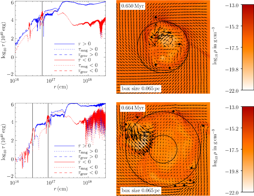
Figure 7.— Torques and density structure. The figure shows cumulative total, magnetic and gravitational torques as function of radius and the gas density $\rho$ in the midplane for two representative snapshots. The magnetic $\tau_{\mathrm{mag}}$ and gravitational torques $\tau_{\mathrm{grav}}$ can reach equipartition locally, but generally the gravitational torque is considerably larger in magnitude. Regions of negative total torques (marked as lines) can be associated with circularly arranged filaments (marked as circles) at the same radii. The black dots represent sink particles. The arrows indicate the direction of the velocity field.

3.4. Gravitational Instability and Fragmentation

The fragmentation of the rotationally flattened accretion flow leads to the formation of relatively long-lived, circularly arranged filaments in run E. This is in contrast to the situation in run B, where the filaments are generally less elongated and their shape and location cannot directly be associated with the rotating flow (see Figure 8). To understand the apparent stability of this structure, we investigate the relative importance of two contributing mechanisms: support by magnetic pressure (Section  3.4.1) and support by strong shear across the filaments (Section 3.4.2).

3.4.1 Support by Magnetic Pressure

Though the magnetic field appears to be not the main driver of negative torques, it is clearly dynamically relevant for the gas dynamics within the accretion flow. This is demonstrated by examining the plasma beta $\beta_{\mathrm{pl}}=p_{\mathrm{th}}/p_{\mathrm{mag}}$ in the midplane, as shown in Figure 8. Outside of the H ii region around the massive star, the magnetic pressure $p_{\mathrm{mag}}$ exceeds the thermal pressure $p_{\mathrm{th}}$ generally, except in the dense filaments. In the central region, $p_{\mathrm{mag}}$ is more than two orders of magnitude larger than $p_{\mathrm{th}}$, but near the filaments $p_{\mathrm{mag}}$ and $p_{\mathrm{th}}$ reach equality.

The plasma beta $\beta_{\mathrm{pl}}$ also quantifies the importance of magnetic support against gravitational collapse in a linear perturbation analysis. The Toomre $Q$-parameter is defined as

$$Q=\frac{\kappa c_{\mathrm{s}}}{\pi\Sigma G}$$ (7)

with epicyclic frequency $\kappa$, sound speed $c_{\mathrm{s}}$, surface density $\Sigma$, and Newton’s gravitational constant $G$. Linear gravitational instability sets in when $Q<1$ (Toomre 1964; Goldreich & Lynden-Bell 1965). When magnetic fields are taken into account (Kim & Ostriker 2001), one can define the magnetic Toomre parameter

$$Q_{\mathrm{M}}=\frac{\kappa\left(c_{\mathrm{s}}^{2}+v_{\mathrm{A}}^{2}\right)^{1/2}}{\pi\Sigma G}$$ (8)

with the Alfvén velocity $v_{\mathrm{A}}$. Since $\beta_{\mathrm{pl}}=c_{\mathrm{s}}^{2}/v_{\mathrm{A}}^{2}$, the ratio of $Q$ and $Q_{\mathrm{M}}$ is

$$\frac{Q_{\mathrm{M}}}{Q}=\sqrt{1+\frac{1}{\beta_{\mathrm{pl}}}}.$$ (9)

Because $\beta_{\mathrm{pl}}$ is larger than unity in the filaments, $Q_{\mathrm{M}}$ and $Q$ only differ by a factor of order unity there, so that magnetic pressure plays no crucial role in stabilizing the filaments.

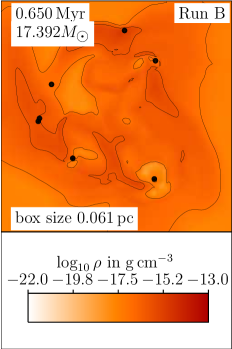
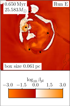
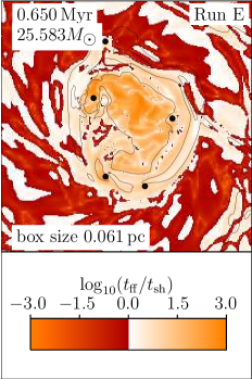
Figure 8.— (Left) Slice of gas density in the hydrodynamical simulation run B. The filaments are much more roundish and are not stretched between rotating and counter-rotating gas. The black dots represent sink particles. The contours show the density structure. (Middle) The plasma beta $\beta_{\mathrm{pl}}=p_{\mathrm{th}}/p_{\mathrm{mag}}$ in the midplane of run E. Outside the H ii region around the $26\,M_{\odot}$ star, the magnetic pressure is generally larger than the thermal pressure and hence is dynamically relevant. However, $p_{\mathrm{th}}$ is slightly larger than $p_{\mathrm{mag}}$ in the filaments, and thus magnetic pressure plays no dominant role in stabilizing them. (Right) The ratio $t_{\mathrm{ff}}/t_{\mathrm{sh}}$ for the same region from run E. The filaments, marked with the density contours, are on the boundary between the stable and the unstable regime.

3.4.2 Support by Shearing Motion

Since the Toomre analysis as presented above only applies to linear perturbations to Keplerian rotation, it entirely neglects the strong shear along the filaments (compare Figure 3). Because the gas on one side of a filament is moving clockwise while the gas on the other side is moving counter-clockwise, there is a large velocity gradient across the filament. This velocity gradient appears able to stabilize the filament. To see how big this effect is, we define the shear timescale

$$t_{\mathrm{sh}}=\frac{1}{|\bm{\nabla}\times\mathbf{v}|}$$ (10)

with the vorticity $\bm{\nabla}\times\mathbf{v}$ and compare this with the free-fall time scale

$$t_{\mathrm{ff}}=\sqrt{\frac{3\pi}{32G\rho}}.$$ (11)

The ratio $t_{\mathrm{ff}}/t_{\mathrm{sh}}$ is plotted in Figure 8. The filaments lie in the marginally stable regime, so that this simple timescale comparison is not totally conclusive. There is, however, a clear difference between the organization of the filaments in run B and run E visible in Figure 8. In run E, the filaments get stretched by the shear and organize circularly, while the filaments in run B are much more roundish in shape. In run E, the filaments separate rotating and counter-rotating gas, which is not generally the case in run B. Since it is the magnetic field that organizes the filaments in this way, the magnetic field indirectly stabilizes the filaments, though not directly through magnetic pressure.

3.5. Relevance for Protostellar Jets

These findings are immediately applicable to the large-scale rotating, infalling flow, far away from the actual radius where high-velocity protostellar jets must be launched. Since the rotation of the launching region determines the outflow velocity, our larger-scale magnetic tower flow, with peak velocities around 5 km s^-1, (compare Figure 4) is slower by a factor of more than 20 than optical jets with velocities exceeding $100\,$km s^-1 (eg. Bally et al. 2007).

However, the behavior seen here may have important implications for understanding the role of jets in high-mass star formation. Such jets are driven from radii of less than an astronomical unit in the accretion disks of low mass stars. We do not resolve the accretion flow to these small radii in our models. However, the huge accretion rates required for high mass star formation suggests that those inner regions must also be highly perturbed and may likely be gravitationally unstable, and thus susceptible to the same fragmentation and destruction of velocity coherence that we have seen in our models. Observations of a counter-rotating accretion disk (Remijan & Hollis 2006) demonstrate that this possibility exists. Simplified one-dimensional calculations (Vaidya et al. 2009) indicate that the temperature may grow strongly enough below a radius of 1 AU to stabilize the disk, but it may be difficult for the magnetic tower to build up on such small scales if the magnetic field outside this radius is totally disarranged. Models of dynamo generation of fields in such disks including non-ideal MHD effects are required to understand whether coherent fields capable of driving jets can form on such small scales. Our findings thus raise the question whether highly collimated, magnetically-driven jets from massive protostars can survive. A negative answer could also explain why outflows from massive stars appear to be less collimated (Arce et al. 2007; Beuther & Shepherd 2005): they are driven by the ionizing radiation instead of coherently rotating magnetic fields. Indeed, Peters et al. (2010a) presented a detailed comparison between the ionization-driven outflows in the purely hydrodynamical simulation with observations of W51e2 and found that the molecular and ionized parts of the outflow have a very similar velocity structure, both qualitatively in the characteristic features as well as quantitatively in the magnitude of the velocity gradient.

3.6. Morphology of H ii Regions

To study the morphological types of the H ii regions in run E in more detail, we have generated synthetic VLA observations at $2\,$cm, following the algorithm described earlier (Peters et al. 2010a, c). Figure 9 shows H ii regions of all morphological types found in run E. There seems to be no systematic difference between the morphologies in the magnetic and purely hydrodynamic simulations (Peters et al. 2010a, c).

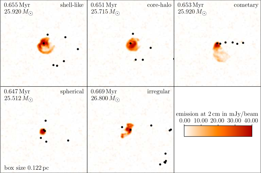
Figure 9.— H ii region morpholgies in run E. The figure shows synthetic maps of free-free emission from ultracompact H ii regions around the massive protostar at different time steps and from different viewing angles. The cluster is assumed to be $2.65\,$kpc away, the full width at half maximum of the beam is $0\hbox{$.\!\!^{\prime\prime}$}14$ and the noise level is $10^{-3}$Jy. This corresponds to typical VLA parameters at a wavelength of $2\,$cm. The protostellar mass of the central star which powers the H ii region is given in the images. Black dots represent sink particles.

Although the magnetic field does not appear to have any influence on the H ii region morphologies themselves, it does play a significant role in determining their size. Figure 10 shows a comparison of thermal and magnetic pressure for the H ii region from Figure 5. The thermal pressure inside the H ii region is of the same order as the magnetic pressure immediately outside the H ii region. Thus, the magnetic pressure yields an important contribution to the total pressure in the environment of the H ii region, constraining its expansion. We therefore expect H ii regions in the presence of strong magnetic fields to be generally smaller than without the magnetic field.

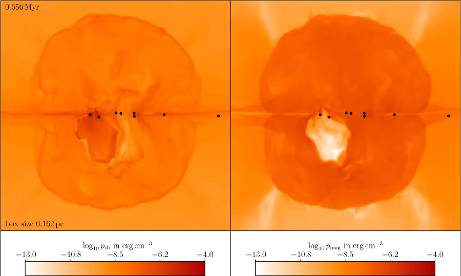
Figure 10.— Comparison of thermal and magnetic pressure for the data from the left-hand panels in Figure 5. The thermal pressure $p_{\mathrm{th}}$ inside the H ii region (left) is of comparable magnitude to the magnetic pressure $p_{\mathrm{mag}}$ outside the H ii region (right). Thus, magnetic pressure plays a significant role in constraining the size of expanding H ii regions. The black dots represent sink particles.

4. Summary and Conclusion

We have presented the first three-dimensional, radiation-magnetohydrodynamical collapse simulation of massive star formation including heating by both ionizing and non-ionizing radiation. We used sink particles to represent accreting protostars. We compared the action of the magnetic field in this high-mass star formation simulation to the major ways that it acts in low-mass star formation. As we summarized in the introduction, these include giving support against gravitational collapse, transferring angular momentum outward, and driving outflows.

We find that, although we started with a mass-to-flux ratio that was more than an order of magnitude supercritical, $(M/\Phi)=14(M/\Phi)_{\mathrm{cr}}$, the magnetic field still can reduce fragmentation (Section 3.1), just as it does in low-mass star formation. The additional magnetic support prevents the gas from collapsing into as many secondary fragments compared to the non-magnetic case, leaving the most massive protostar with a larger gas reservoir. For the same reason, the total accretion rate is reduced. However, it is important to note that the magnetic field does not suppress fragmentation completely. The number of fragments is reduced at most by a factor of two. Similar findings are reported by Hennebelle et al. (2010, A&A, submitted).

Additionally, magnetic braking near the center reduces the angular momentum of the collapsing gas even further. Thus, more material is transported radially inwards onto the massive central protostar. This is important since the distribution of mass accretion among the protostars in the fragmentation-induced starvation scenario depends sensitively on the (in)efficiency of gas transport towards the center by internal torques (Peters et al. 2010a, b).

The combination of these two effects causes the formation of a 50% more massive central star compared to our equivalent simulation without magnetic fields (Figure 1c). If the magnetic field strengths inferred by Falgarone et al. (2008) are typical throughout high-mass clumps, and not just in their high-density cores, magnetic braking and reduction of fragmentation may be even stronger than reported here.

The winding up of the magnetic field into a toroidal configuration leads to the formation of a large-scale tower flow, surrounding all the protostars. However, two effects tend to weaken and broaden the outflow. The first one is the gravitational fragmentation of the accretion flow. This disrupts the circular motion necessary to drive the tower flow in the central region. Second, the thermal pressure of ionized gas is by far larger than the magnetic pressure and hence dynamically dominant within the H ii region. The resulting expansion of the H ii region dramatically reduces the magnetic energy content within it, and tangles the field lines, further weakening the flow.

The torques required to brake the large-scale rotating flow and reverse the azimuthal velocity are primarily gravitational, though magnetic and gravitational torques can reach equipartition locally. Magnetic braking appears to be of minor importance for the global gas dynamics, but not necessarily for the local accretion onto protostars. Again, if stronger magnetic fields are imposed, magnetic braking might become qualitatively more important. The shape and dynamics of the filaments is vastly different in the magnetohydrodynamical (run E) and purely gas dynamical (run B) case: while the filaments in run B are disorganized, roundish and quickly collapse to form stars, the filaments in run E are stretched between clockwise and counter-clockwise rotating gas and can be maintained over a large fraction of the simulation runtime.

If the fragmentation process observed in our simulations holds down to the smallest scales of the massive accretion disk, as suggested by the very high accretion rates of the order $10^{-3}\,M_{\odot}\,$yr^-1 inevitably needed to form a massive star, the magnetic field can only wind up at radii less than 1 AU, where the temperature is high enough to suppress gravitationl instability of the disk (Vaidya et al. 2009). In this case, magnetically-driven, steady jets around massive protostars can only survive until gravitational fragmentation disrupts uniform rotation, and ionizing radiation becomes dynamically relevant. We call this process fragmentation-induced outflow disruption. The fast jets launched from the inner disk region should then be highly episodic like the accretion rates. The uncollimated outflows from massive stars may be better explained as driven by the ionization feedback.

References

- Arce et al. (2007) Arce, H. G., Shepherd, D., Gueth, F., Lee, C.-F., Bachiller, R., Rosen, A., & Beuther, H. 2007, in Protostars and Planets V, ed. B. Reipurth, D. Jewitt, & K. Keil (The University of Arizona Press), 245–260
- Bachiller (1996) Bachiller, R. 1996, ARA&A, 34, 111
- Balbus & Hawley (1991) Balbus, S. A. & Hawley, J. F. 1991, ApJ, 376, 214
- Balbus & Hawley (1998) —. 1998, Rev. Mod. Phys., 70, 1
- Bally et al. (2007) Bally, J., Reipurth, B., & Davis, C. J. 2007, in Protostars and Planets V, ed. B. Reipurth, D. Jewitt, & K. Keil (The University of Arizona Press), 215–230
- Banerjee & Pudritz (2006) Banerjee, R. & Pudritz, R. E. 2006, ApJ, 641, 949
- Banerjee & Pudritz (2007) —. 2007, ApJ, 660, 479
- Basu & Mouschovias (1994) Basu, S. & Mouschovias, T. C. 1994, ApJ, 432, 720
- Beuther et al. (2002) Beuther, H., Schilke, P., Sridharan, T. K., Menten, K. M., Walmsley, C. M., & Wyrowski, F. 2002, A&A, 383, 892
- Beuther & Shepherd (2005) Beuther, H. & Shepherd, D. 2005, in Cores to Clusters: Star Formation with Next Generation Telescopes, ed. M. S. N. Kumar, M. Tafalla, & P. Caselli (Springer-Verlag), 105–119
- Blandford & Payne (1982) Blandford, R. D. & Payne, D. G. 1982, MNRAS, 199, 883
- Bürzle et al. (2010) Bürzle, F., Clark, P. C., Stasyszyn, F., Greif, T., Dolag, K., Klessen, R. S., & Nielaba, P. 2010, ArXiv:1008.3790
- Cabrit & André (1991) Cabrit, S. & André, P. 1991, ApJ, 379, L25
- Cai et al. (2008) Cai, M. J., Shang, H., Lin, H.-H., & Shu, F. H. 2008, ApJ, 672, 489
- Commerçon et al. (2010) Commerçon, B., Hennebelle, P., Audit, E., Chabrier, G., & Teyssier, R. 2010, A&A, 510, L3
- Crutcher (2009) Crutcher, R. M. 2009, Rev. Mex. Astron. Astrofís., 36, 107
- Crutcher (2010) Crutcher, R. M. 2010, in http://www.mpia-hd.mpg.de/homes/stein/EPoS/Onlinematerial/crutcher.pdf.gz, ed. J. Steinacker & A. Bacmann
- Falgarone et al. (2008) Falgarone, E., Troland, T. H., Crutcher, R. M., & Paubert, G. 2008, A&A, 487, 247
- Federrath et al. (2010) Federrath, C., Banerjee, R., Clark, P. C., & Klessen, R. S. 2010, ApJ, 713, 269
- Ferreira et al. (2006) Ferreira, J., Dougados, C., & Cabrit, S. 2006, A&A, 453, 785
- Fryxell et al. (2000) Fryxell, B., Olson, K., Ricker, P., Timmes, F. X., Zingale, M., Lamb, D. Q., MacNeice, P., Rosner, R., Truran, J. W., & Tufo, H. 2000, ApJS, 131, 273
- Galli & Shu (1993a) Galli, D. & Shu, F. H. 1993a, ApJ, 417, 220
- Galli & Shu (1993b) —. 1993b, ApJ, 417, 243
- Goldreich & Lynden-Bell (1965) Goldreich, P. & Lynden-Bell, D. 1965, MNRAS, 130, 97
- Heiles (1976) Heiles, C. 1976, ARA&A, 14, 1
- Hennebelle & Ciardi (2009) Hennebelle, P. & Ciardi, A. 2009, A&A, 506, L29
- Hennebelle & Fromang (2008) Hennebelle, P. & Fromang, S. 2008, A&A, 477, 9
- Hennebelle & Teyssier (2008) Hennebelle, P. & Teyssier, R. 2008, A&A, 477, 25
- Keto & Wood (2006) Keto, E. & Wood, K. 2006, ApJ, 637, 850
- Kim & Ostriker (2001) Kim, W.-T. & Ostriker, E. C. 2001, ApJ, 559, 70
- Kim et al. (2003) Kim, W.-T., Ostriker, E. C., & Stone, J. M. 2003, ApJ, 599, 1157
- Königl & Pudritz (2000) Königl, A. & Pudritz, R. E. 2000, in Protostars and Planets IV, ed. V. Mannings, A. P. Boss, & S. S. Russell (The University of Arizona Press), 759–787
- Krumholz & McKee (2008) Krumholz, M. R. & McKee, C. F. 2008, Nature, 451, 1082
- Lada (2006) Lada, C. J. 2006, ApJ, 640, L63
- Lovelace et al. (1999) Lovelace, R. V. E., Romanova, M. M., & Bisnovatyi-Kogan, G. S. 1999, ApJ, 514, 368
- Mac Low & Klessen (2004) Mac Low, M.-M. & Klessen, R. S. 2004, Rev. Mod. Phys., 76, 125
- Mac Low et al. (1998) Mac Low, M.-M., Klessen, R. S., Burkert, A., & Smith, M. D. 1998, Phys. Rev. Lett., 80, 2754
- Machida et al. (2004) Machida, M. N., Tomisaka, K., & Matsumoto, T. 2004, MNRAS, 348, L1
- Matsumoto & Hanawa (2010) Matsumoto, T. & Hanawa, T. 2010, arxiv:1008.3984
- Matsumoto & Tomisaka (2004) Matsumoto, T. & Tomisaka, K. 2004, ApJ, 616, 266
- McKee & Tan (2003) McKee, C. F. & Tan, J. C. 2003, ApJ, 585, 850
- Mouschovias (1991) Mouschovias, T. C. 1991, in The Physics of Star Formation and Early Stellar Evolution, ed. C. J. Lada & N. D. Kylafis (Kluwer Academic Publishers Group), 61–122
- Mouschovias & Paleologou (1979) Mouschovias, T. C. & Paleologou, E. V. 1979, ApJ, 230, 204
- Mouschovias & Paleologou (1980) —. 1980, ApJ, 237, 877
- Mouschovias & Spitzer (1976) Mouschovias, T. C. & Spitzer, Jr., L. 1976, ApJ, 210, 326
- Mueller et al. (2002) Mueller, K. E., Shirley, Y. L., Evans, II, N. J., & Jacobson, H. R. 2002, ApJS, 143, 469
- Najita & Shu (1994) Najita, J. R. & Shu, F. H. 1994, ApJ, 429, 808
- Peters et al. (2010a) Peters, T., Banerjee, R., Klessen, R. S., Mac Low, M.-M., Galván-Madrid, R., & Keto, E. R. 2010a, ApJ, 711, 1017
- Peters et al. (2010b) Peters, T., Klessen, R. S., Mac Low, M.-M., & Banerjee, R. 2010b, ApJ, 725, 134
- Peters et al. (2010c) Peters, T., Mac Low, M.-M., Banerjee, R., Klessen, R. S., & Dullemond, C. P. 2010c, ApJ, 719, 831
- Price & Bate (2007) Price, D. J. & Bate, M. R. 2007, MNRAS, 377, 77
- Reipurth & Bally (2001) Reipurth, B. & Bally, J. 2001, ARA&A, 39, 403
- Remijan & Hollis (2006) Remijan, A. J. & Hollis, J. M. 2006, ApJ, 640, 842
- Rijkhorst et al. (2006) Rijkhorst, E.-J., Plewa, T., Dubey, A., & Mellema, G. 2006, A&A, 452, 907
- Romanova et al. (2009) Romanova, M. M., Ustyugova, G. V., Koldoba, A. V., & Lovelace, R. V. E. 2009, MNRAS, 399, 1802
- Shu et al. (1994) Shu, F., Najita, J., Ostriker, E., Wilkin, F., Ruden, S., & Lizano, S. 1994, ApJ, 429, 781
- Shu et al. (2007) Shu, F. H., Galli, D., Lizano, S., & Cai, M. J. 2007, in Star-disk interaction in young stars, ed. J. Bouvier & I. Appenzeller, IAU Symposium No. 243 (Cambridge University Press), 249–264
- Strittmatter (1966) Strittmatter, P. A. 1966, MNRAS, 132, 359
- Tomida et al. (2010) Tomida, K., Tomisaka, K., Matsumoto, T., Ohsuga, K., Machida, M. N., & Saigo, K. 2010, ApJ, 714, L58
- Tomisaka (1998) Tomisaka, K. 1998, ApJ, 502, L163
- Tomisaka (2002) —. 2002, ApJ, 575, 306
- Toomre (1964) Toomre, A. 1964, ApJ, 139, 1217
- Uchida & Shibata (1985) Uchida, Y. & Shibata, K. 1985, PASJ, 37, 515
- Vaidya et al. (2009) Vaidya, B., Fendt, C., & Beuther, H. 2009, ApJ, 702, 567
- Waagan (2009) Waagan, K. 2009, J. Comput. Phys., 228, 8609
- Wang et al. (2010) Wang, P., Li, Z.-Y., Abel, T., & Nakamura, F. 2010, ApJ, 709, 27
- Ziegler (2005) Ziegler, U. 2005, A&A, 435, 385
- Zinnecker & Yorke (2007) Zinnecker, H. & Yorke, H. W. 2007, ARA&A, 45, 481