Magnetic field dependence and the possibility of filtering ultraslow light pulses in atomic gases with Bose Einstein condensates

Abstract

This paper studies theoretically the ultraslow light phenomenon in Bose Einstein condensates of alkali-metal atoms. The description is based on the linear approach that is developed in the framework of the Green function formalism. It is pointed out that the group velocity of light pulses that are tuned up close to resonant lines of the alkali atoms’ spectrum may strongly depend on the intensity of the external static magnetic field. The possibility of filtering optical pulses using the ultraslow light phenomenon in Bose condensates is discussed.

1 Introduction

Bose-Einstein condensate (BEC) is one of the most impressive examples when the matter demonstrates its quantum nature on the macroscopic level. Now this system is interesting also due to the possibility to observe the electromagnetic pulses propagating with extremely slow group velocities in it [1]. Evidently, the choice of alkali-metal vapors corresponds to the fact that a behavior of a many-particle system consisting of alkali metals is more predictable and convenient from the standpoint of quantum mechanics than a behavior of the system consisting of atoms with more complicated structure. The main reason for that is a hydrogenlike structure of alkali metals. Therefore, the energy spectrum of these atoms and interaction peculiarities with an external electromagnetic field are well-studied to the present moment.

For the many-particle system consisting of alkali atoms one can construct rather exact microscopic description, which includes the effects of collective interaction of these systems with electromagnetic waves. This description is based on an approximate formulation of the second quantization method [2] in the case of a presence of bound states of particles. In the framework of this formulation one may consider alkali metals as bound states of two ”elementary” particles: the valence electron and the atomic core. This method allows not to consider an atom as a compound particle, but describe it as an elementary object with preserving the information relating to its internal degrees of freedom (wave functions, energy spectrum, etc).

On the basis of the developed microscopic approach in Refs. [3, 4, 5] it was studied the response of a system to an external electromagnetic perturbation in the framework of the Green-function formalism. In terms of the Green functions the expressions for the permittivity and magnetic permeability of an ideal gas of hydrogenlike atoms with a Bose condensate. It was found that the permittivity demonstrates the resonance behavior at frequencies close to the allowed transitions between certain quantum states of an atom. Note that this behavior of the permittivity is well-known from the classical approaches [6]. But, the proposed theory allows to estimate the values of all microscopic quantities that appear in the expressions characterizing the response of a gas with a BEC.

It it easy to see that the energy spacing between different states of an atom can strongly depend on the intensity of an external magnetic field. Aside the cases, in which this field can be specially turned on, it can appear due to the usage of magneto-optical traps and bias fields in BEC-related experiments. The mentioned dependence of the energy spectrum on the magnetic field corresponds to the Zeeman splitting (or the Paschen-Back splitting) of the ground and excited states of an atom. In turn, the resonance behavior of the refractive index is one of the necessary conditions for the pulses slowing in a Bose condensate [4]. Thus, one can expect that by the change of the intensity of a bias field it is possible to control the propagation velocity and to filter light pulses that propagate through a BEC cloud.

2 Linear response of a gas to an external probe radiation

Firstly, it should be noted that in the present paper the description is based on the weak-field approximation. In other words, it is assumed that an external electromagnetic field (laser pulse) is probe and practically do not influence on the occupation of the states in the system. This limitation is necessary for the usage of the results of the linear-response theory, which is based on the Green-functions formalism [7]. The mentioned fact excludes the possibility to describe the influence of an additional coupling laser (quantum interference effects) on the system under consideration. Note that the coupling field was used in the experiment [1] to provide an electromagnetically-induced transparency (EIT) at the resonance regions. But, as it is shown in Ref. [4], the usage of quantum interference effects is not a necessary condition for the pulses slowing. Moreover, the coupling field may influence on the energy spectrum of the atoms. Thus, it inevitably produce additional difficulties in the construction of the description.

Usually, for the achievement of the BEC regime in the systems consisting of alkali-metal atoms, the dilute vapors with the density of particles $\nu\lesssim 10^{14}$ cm^-3 are used. These vapors with a good precision can be considered as ideal gases [8]. Hence, to describe microscopically the propagation of electromagnetic pulses in this medium, it is convenient to use the results [4]. There it was shown that the expression for the permittivity of the gas in the BEC state can be written as follows:

$$\epsilon^{-1}(\textbf{k},\omega)\approx 1+\frac{4\pi}{k^{2}}\sum\limits_{\alpha,\beta}\frac{(\nu_{\alpha}-\nu_{\beta})|\sigma_{\alpha\beta}(\textbf{k})|^{2}}{\omega+\Delta\varepsilon_{\alpha\beta}+i\gamma_{\alpha\beta}},$$ (1)

where $\omega$, k are the frequency and wave vector of the external field (probe laser), $\nu_{\alpha}$ is the density of condensed atoms in the $\alpha$ quantum state, $\Delta\varepsilon_{\alpha\beta}$ is the energy interval between the $\alpha$ and $\beta$ states, and $\gamma_{\alpha\beta}$ is the linewidth related to the probability of a spontaneous transition between these states. The quantity $\sigma_{\alpha\beta}(\textbf{k})$ is the matrix element of the charge density, which is defined by the relation

$$\sigma_{\alpha\beta}(\textbf{k})=e\int d\textbf{y}\varphi_{\alpha}^{*}(\textbf{y})\varphi_{\beta}(\textbf{y})\left[\exp{\left(i\frac{m_{p}}{m}\textbf{k}\textbf{y}\right)}-\exp{\left(-i\frac{m_{e}}{m}\textbf{k}\textbf{y}\right)}\right],$$ (2)

where $\varphi_{\alpha}(\textbf{y})$ is the atomic wave function in the $\alpha$ state, $e$ is the electron charge absolute value, $m_{p}$ and $m_{e}$ are the masses of the atomic core and electron, respectively ($m=m_{p}+m_{e}$). In the case of the allowed dipole transitions, in the linear order over $(\textbf{ky})\ll 1$, one gets

$$\sigma^{(1)}_{\alpha\beta}(\textbf{k})\approx i\textbf{k}\textbf{d}_{\alpha\beta},\quad\textbf{d}_{\alpha\beta}=e\int\textbf{y}d\textbf{y}\varphi_{\alpha}^{*}(\textbf{y})\varphi_{\beta}(\textbf{y}),$$ (3)

where $\textbf{d}_{\alpha\beta}$ denotes the atomic dipole moment, which is related to the transition $\alpha\leftrightarrow\beta$.

Considering that the density of the excited atoms is negligibly small in comparison with the density of atoms in the ground state (the case of a low intensity of the probe laser), one can neglect of the second term in Eq. (1). Therefore, one gets the expression

$$\epsilon^{-1}(\textbf{k},\omega;B)\approx 1+\sum\limits_{\alpha,\beta}{a_{\alpha\beta}}\left[\omega+\Delta\varepsilon_{\alpha\beta}(B)+i\gamma_{\alpha\beta}\right]^{-1}.$$ (4)

Here the set of quantum numbers of ground and excited state are denoted by the $\alpha$ and $\beta$ indexes, respectively. As in this paper the limit of zero temperatures is considered, the quantity $\gamma_{\alpha\beta}$ corresponds to the probability of a spontaneous transition between the $\beta$ and $\alpha$ states. Note that by the term ”ground state of an atom” relates to all sublevels of the ground state (for alkali metals these levels have zero orbital number), which are splitted by the hyperfine and Zeeman interaction. According to Eqs. (1) and (3), the quantity in Eq. (4)

$$a_{\alpha\beta}=4\pi\nu_{\alpha}d_{\alpha\beta}^{2}/3$$ (5)

defines the dependence of dispersion characteristics on the atomic polarization and the density of atoms in the BEC state. Note also that the dependence of dispersion characteristics on the intensity of a static magnetic field $B$ (see Eq. (4)) is mainly defined by the energy interval $\Delta\varepsilon_{\alpha\beta}(B)$ between corresponding ground and excited states of an atom. Thus it is necessary to study dependencies of the resonant transitions on the field intensity in detail.

3 Hyperfine structure of the sodium D₂ line in the external magnetic field

Now it is important to obtain the energy spectrum of alkali-metal atoms in the presence of a magnetic field with account of the hyperfine interaction. To this end, one should consider the following Hamiltonian (see also Ref. [9]):

$$\hat{V}=A_{hfs}\hat{\textbf{I}}\cdot\hat{\textbf{J}}+B_{hfs}\hat{Q}+\mu_{B}(g_{I}\hat{I}_{z}+g_{J}\hat{J}_{z})B,$$ (6)

where $A_{hfs}$ and $B_{hfs}$ are the hyperfine constants related to the magnetic dipole and electric quadrupole interaction of the nucleus and valence electron, respectively ($B_{hfs}=0$ for the states $J=1/2$). The quantities $\hat{\textbf{I}}$ and $\hat{\textbf{J}}$ are the operators of the nucleus and electron total angular momentum, respectively, $\hat{I}_{z}$ and $\hat{J}_{z}$ are the operators of the projections of these operators on the magnetic field $B$ direction, $\mu_{B}$ is the Bohr magneton (in the units $\hbar=1$), and $g_{I}$ and $g_{J}$ are corresponding Landé factors. The operator $\hat{Q}$ can be expressed in terms of the operators $\hat{\textbf{I}}$ and $\hat{\textbf{J}}$ as follows:

$$\hat{Q}=\frac{3(\hat{\textbf{I}}\cdot\hat{\textbf{J}})^{2}+\frac{3}{2}\hat{\textbf{I}}\cdot\hat{\textbf{J}}-I(I+1)J(J+1)}{2I(2I-1)2J(2J-1)}.$$ (7)

Note that for the splitted levels of the ground state the spectrum can be found analytically. At the same time, for the excited levels (triple and more degenerated states in the total momentum projection $m_{F}$, $\hat{\textbf{F}}=\hat{\textbf{I}}+\hat{\textbf{J}}$) it is rather difficult to find corresponding analytical expressions. But in this case one can find it numerically. One may verify that the limiting cases of the numerical results lie in a good agreement with the analytical formulas.

By the example of a sodium atom, it is possible to study the dependence of $D_{2}$-line components on the magnetic field in detail. This line corresponds to the transition between the 3$S_{1/2}$-state sublevels and 3$P_{3/2}$-state sublevels. It is not difficult to obtain the Zeeman splitting of these levels with account of the hyperfine interaction (see Eqs. (6) and (7)) as it is done in Ref. [9]. As one can see, the resonant $D_{2}$ line splits to a large number of components. Each component can be found from the difference between corresponding excited and ground state with the use of the selection rule for the quantum numbers $F$ and $m_{F}$ ($\Delta F=0,\pm 1$; $\Delta m_{F}=0,\pm 1$).

Usually, depending on $\Delta m_{F}$ value, one can say about linearly or $\pi$-polarized transitions ($\Delta m_{F}=0$), and circularly or $\sigma^{\pm}$-polarized transitions, $\Delta m_{F}=\pm 1$ [6]. Note that in the experiments with ultraslow light the laser with the certain polarization is used. Thus, one needs to consider the transitions between the states of an atom corresponding to the certain polarization. Hence, in the next calculations the response of the system to the linearly-polarized pulse is considered. For this radiation the resonance frequencies correspond to the transitions $\Delta F=0,\pm 1$; $\Delta m_{F}=0$). The magnetic-field dependence for these components can be found from the dependencies for the Zeeman splitting of the ground and excited states (see, e.g., Ref. [5]). Accounting the mentioned selection rules, one can find the dependencies for the ”upper” $\pi$-transitions (transitions from the ground state with $F=2$) that are shown in Fig. 1.

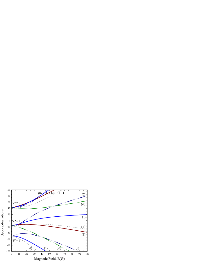
Figure 1: Components of the sodium $D_{2}$ line in the external static magnetic field ($F=2$; $\Delta F=0,\pm 1$; $\Delta m_{F}=0$). The number in brackets corresponds to the momentum projection $m_{F}$ of the quantum state.

4 Dependence of the group velocity on the magnetic field intensity

Now one can conclude that at certain intensities of magnetic fields at the same frequency two different transitions are possible (regions of the lines intersection, see Fig. 1). These regions may be very interesting from the standpoint of the experiments related to the ultraslow-light phenomenon. The reason is that the value of the group velocity depends on the dispersion characteristics of the medium. In particular, it depends on the derivative of the refractive index by the frequency. Note that the smaller the difference between two resonant frequencies, the narrower the spacing between corresponding peaks of the refractive index, and the steepness of the slope is larger. But this characteristic does not mean that in the region of intersection one should expect the maximal reduction of the group velocity. In this case, the natural linewidth of the excited state component (sublevel) plays an essential role. These quantities for the excited sublevels can be obtained from the relative hyperfine transition strength factors $S_{FF^{\prime}}$ [9], $\gamma_{FF^{\prime}}=S_{FF^{\prime}}\Gamma_{e}/2$, where for sodium atom $\Gamma_{e}=9.795$ MHz. For example, if the atoms are prepared in the ground states with $F=2$, one must take corresponding strength factors for the ”upper” transitions (see Fig. 1), $S_{21}=1/20$, $S_{22}=1/4$, and $S_{23}=7/10$.

Next, analyzing dependencies that are shown in Fig. 1, one can choose the frequency of the linear-polarized light close to the lowest intersection of the eigenfrequencies $\omega_{1}$ (dotted line in the lower part denoted by (0)) and $\omega_{2}$ (dotted line in the lower part denoted by (-2)). In particular, it is convenient to take $\omega^{(e)}=\omega_{0}+\Delta$, where $\omega_{0}$ is $D_{2}$-line resonance frequency without account of the hyperfine interaction ($\omega_{0}=508.848716$ THz), and $\Delta$ is the chosen detuning ($\Delta=-45.0$ MHz). It is also necessary to consider that two corresponding ground-state sublevels are occupied (quantum states $|1\rangle=|F=2,m_{F}=0\rangle$ and $|2\rangle=|F=2,m_{F}=-2\rangle$). In this case one can simplify calculations by accounting only two resonant summands in (4). Really, as one can conclude from Fig. 1, in this case the major role play the transitions corresponding to the eigenfrequencies $\omega_{1}$ and $\omega_{2}$. Therefore, one gets rather simple expression for the permittivity,

$$\epsilon^{-1}(\textbf{k},\omega;B)\approx 1+\sum\limits_{j=1}^{2}{a_{j}}[\omega-\omega_{j}(B)+i\gamma_{j}]^{-1}.$$ (8)

where the quantities $\gamma_{j}=S_{FF^{\prime}}\Gamma_{e}/2$, $a_{j}=4\pi\nu_{j}d_{FF^{\prime}}^{2}/3$ (see Eq. (5)), $d_{FF^{\prime}}^{2}\approx S_{FF^{\prime}}(3.52er_{0})^{2}$ [9], $r_{0}$ is the Bohr radius, and $e$ is the elementary charge. The summand $j=1$ in this case corresponds to the transition quantum numbers $F=2$, $F^{\prime}=1$ and the summand $j=2$ corresponds to $F=2$, $F^{\prime}=2$.

By introducing the real and imaginary parts of the permittivity ($\epsilon^{\prime}$ and $\epsilon^{\prime\prime}$, respectively) it is easy to find the relations defining the refractive index and damping factor quantities: $\epsilon^{\prime}=n^{\prime 2}-n^{\prime\prime 2}$ and $\epsilon^{\prime\prime}=2n^{\prime}n^{\prime\prime}$. In the transmission region the refractive index $n^{\prime}$ defines the group velocity of the signal, and the damping factor $n^{\prime\prime}$ defines the intensity of the transmitted light,

$$v_{g}(\omega,B)=c\left\{n^{\prime}(\omega,B)+\omega[\partial n^{\prime}(\omega,B)/\partial\omega]\right\}^{-1},$$ (9)

$$I(\omega,B)=I_{0}(\omega)\exp{[-n^{\prime\prime}(\omega,B)kL]},$$ (10)

where $I_{0}(\omega)$ is the spectral density of the initial pulse, $L$ is the characteristic linear size of a condensed cloud.

Next, by setting $\omega=\omega^{(e)}$, $\nu_{1}=\nu_{2}=2\times 10^{10}$ cm^-3, and $L=0.004$ cm, it is easy to calculate the quantities (9) and (10) for the different values of the intensity of a bias field. By the use of these results one can get the dependencies that are shown in Fig. 2.

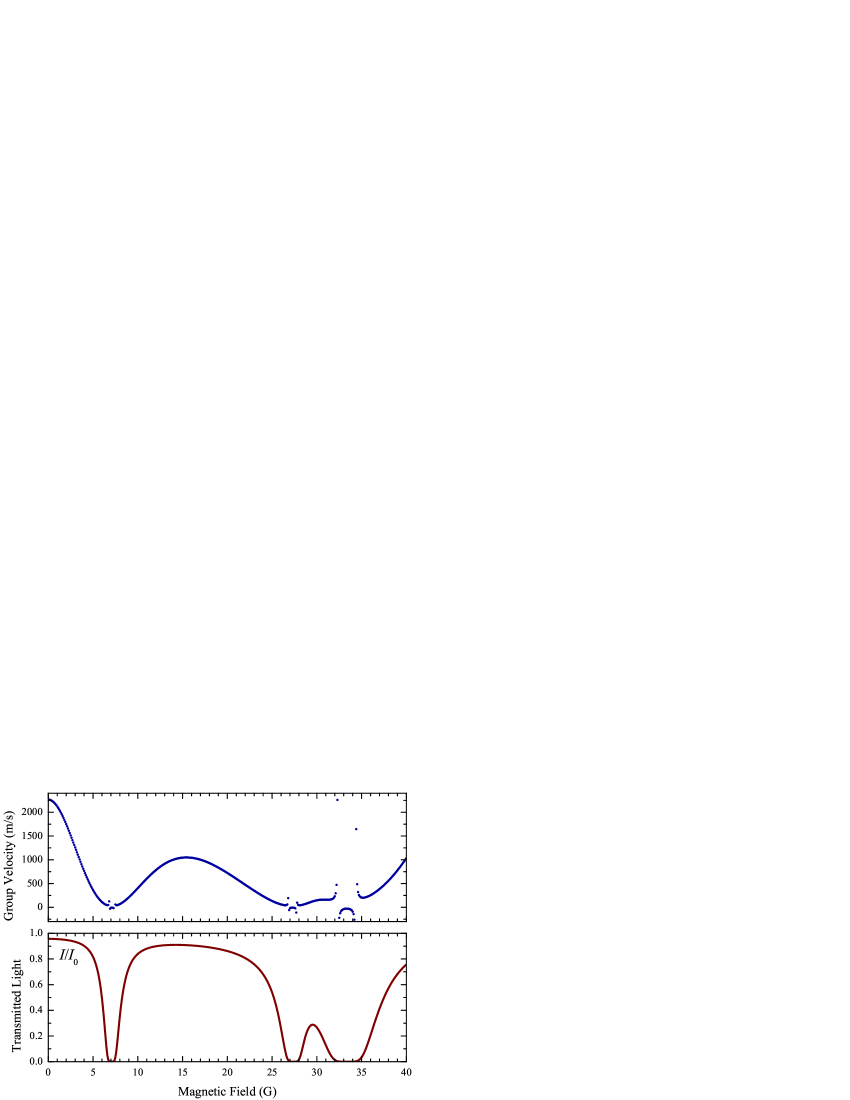
Figure 2: Dependencies of the group velocity and relative intensity on the external static magnetic field for the resonant light pulses with the constant detuning $\Delta=-45.0$ MHz.

As it is easy to see, these dependencies have a rather nontrivial form. One can conclude that in some regions the velocity can be reduced more than in ten times by the change of the field intensity only in several gauss. Moreover, in some regions ($|\omega^{(e)}-\omega_{i}|<\gamma_{i}$) the group velocity has negative values. But, as it is shown in the lower part of Fig. 2, in these regions the signal is mostly absorbed. The absorption rate can be made much lower by the use of a gas with the lower density or with smaller characteristic size $L$. In this case one should observe the light pulses propagating in a BEC with a negative group velocity. Note also that the propagation of the light pulses with a negative group velocity for similar systems is well-studied both theoretically and experimentally (see Ref. [10] for details).

5 Possibility to filter the signals by the use of the ultraslow-light phenomenon in a BEC

To show a possibility to filter optical pulses in a BEC in the presence of the external static magnetic field it is convenient to choose some model. In particular, when the spectral density of the initial pulse has a normal (Gaussian) distribution, it can be written as follows:

$$I_{0}(\omega)=\frac{I_{0}}{\sigma\sqrt{2\pi}}\exp\left[-(\omega-\omega_{0})^{2}/2\sigma^{2}\right].$$ (11)

To get appreciable results, it is convenient to choose $\omega_{0}=508.848052$ THz, $\sigma=50$ MHz (the signal can effectively interact with several hyperfine components of the sodium D₂ line, see Fig. 1), and the linear polarization of the signal.

Next, it is necessary to choose the gas properties. For example, one can take the gas of sodium atoms with two occupied ground states: $|1\rangle=|F=2,m_{F}=1\rangle$ and $|2\rangle=|F=2,m_{F}=2\rangle$. The resonant transitions dependencies on the magnetic field for these states are marked by solid bold lines in Fig. 1. Next, taking for the convenience $\nu_{1}=\nu_{2}=10^{12}$ cm^-3, $B=25$ G, and $L=40~{}\mu$m, in accordance with Eqs. (9) and (10), one can get the dependencies that are shown in Fig. 3.

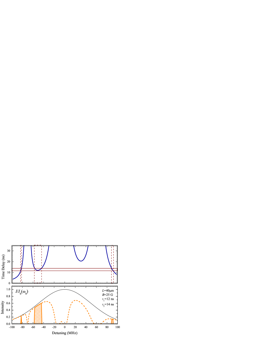
Figure 3: Frequency dependencies of the time delay and relative intensity of the signal that propagates through a condensed gas with the occupied states $|F=2,m_{F}=1\rangle$ and $|F=2,m_{F}=2\rangle$.

Therefore, from Fig. 3 one can see that different parts of the pulse have different time delays resulting from the fact that the group velocity of these parts in gas a with condensates has different values due to the ultraslow-light phenomenon. It should be noted that that at certain frequencies the signal is mostly absorbed by medium. But this is not enough (see dashed line in the lower part of Fig. 3) to reach good parameters for filtering optical pulses. One needs also to use additional techniques for a registration of the signal only in the certain time interval. As it easy to see from Fig. 3 (bold solid line in the lower part corresponds to the time interval from 12 to 14 ns), by the use of the mentioned method one can get filtered pulses with relatively good parameters.

In conclusion, it is important to note that the cases, which is studied in this paper, is demonstrative in some sense. In the framework of the proposed approach one can obtain the results for another polarizations, occupied states, another frequency detunings, and also another types of alkali atoms. Evidently, this fact expands the possibility for the experimental observation of the effects that are studied in this work.

References

References

- [1] L. V. Hau, S. E. Harris, Z. Dutton, C. H. Behroozi, Nature 397, 594 (1999).
- [2] S. V. Peletminskii, Y. V. Slyusarenko, J. Math. Phys. 46, 022301 (2005).
- [3] Y. V. Slyusarenko, A. G. Sotnikov, Condens. Matter Phys. 9, 459 (2006).
- [4] Y. Slyusarenko, A. Sotnikov, Phys. Rev. A 78, 053622 (2008).
- [5] Y. Slyusarenko, A. Sotnikov, Phys. Lett. A 373, 1392 (2009).
- [6] M. O. Scully, M. S. Zubairy, Quantum Optics (Cambridge University Press, Cambridge, 2002).
- [7] A. I. Akhiezer, S. V. Peletminskii, Methods of statistical physics (Pergamon Press, Oxford, 1981).
- [8] L. P. Pitaevskii, S. Stringari, Bose-Einstein Condensation (Clarendon Press, Oxford, 2003).
- [9] D. Steck, http://steck.us/alkalidata.
- [10] B. Ségard, B. Macke, Eur. Phys. J. D 23, 125 (2003).