Thermally assisted spin transfer torque switching in synthetic free layers

Abstract

We studied the magnetization reversal rates of thermally assisted spin transfer torque switching in a synthetic free layer theoretically. By solving the Fokker-Planck equation, we obtained the analytical expression of the switching probability for both the weak and the strong coupling limit. We found that the thermal stability is proportional to $\Delta_{0}(1-I/I_{\rm c})^{2}$, not $\Delta_{0}(1-I/I_{\rm c})$ as argued by Koch et al. [Phys. Rev. Lett. ${\bm{9}2}$, 088302 (2004)], where $I$ and $I_{\rm c}$ are the electric current and the critical current of spin transfer torque switching at absolute zero temperature, respectively. The difference in the exponent of $(1-I/I_{\rm c})$ leads to a significant underestimation of the thermal stability $\Delta_{0}$. We also found that fast switching is achieved by choosing the appropriate direction of the applied field.

I Introduction

Spin transfer torque switching of the magnetization in ferromagnetic nanostructures has been extensively studied both theoretically Slonczewski (1989, 1996); Berger (1996) and experimentally Katine et al. (2000); Kiselev et al. (2003); Huai et al. (2004); Fuchs et al. (2004) because of its potential application to spin-electronics devices such as magnetic random access memory. For device applications, a thermal stability $\Delta_{0}=MH_{\rm an}V/(2k_{\rm B}T)$ of more than 40 is required to guarantee retention time of longer than ten years, where $M$, $H_{\rm an}$, $V$, $k_{\rm B}$ and $T$ are the magnetization, the anisotropy field, the volume of the free layer, the Boltzmann constant, and the temperature, respectively.

Recently, Hayakawa et al. Hayakawa et al. (2008) showed that the anti-ferromagnetically coupled synthetic free layer, CoFeB(2.6nm)/Ru(0.8nm)/CoFeB(2.6nm), in a CoFeB(fixed layer)/MgO/CoFeB/Ru/CoFeB magnetic tunnel junction shows a large thermal stability ($\Delta_{0}>80$) compared to a single free layer. On the other hand, Yakata et al. Yakata et al. (2009, 2010) showed that a ferromagnetically coupled CoFeB/Ru/CoFeB synthetic free layer shows a large thermal stability ($\Delta_{0}=146\pm 29$ for CoFeB(2nm)/Ru(1.5nm)/CoFeB(2nm) and $248\pm 60$ for CoFeB(2nm)/Ru(1.5nm)/CoFeB(4nm)) compared to the single and the anti-ferromagnetically coupled synthetic free layer. These intriguing results spurred us to study a thermally assisted spin transfer torque switching in synthetic free layer. In contrast to the large number of experimental studies Hayakawa et al. (2008); Yakata et al. (2009, 2010), few theoretical studies have been reported. Although the analytical expression of the switching rate of the thermally assisted spin transfer torque switching for the single free layer Koch et al. (2004); Li and Zhang (2004); Apalkov and Visscher (2005), $P=1-\exp[-f_{0}t\exp\{-\Delta_{0}(1-I/I_{\rm c})(1-H_{\rm appl}/H_{\rm an})^{2}\}]$, has been widely used to fit the experiments [see Eqs. (1)-(3) in Refs. Yakata et al. (2009, 2010)], where $I_{\rm c}$ is the critical current of the spin transfer torque switching at absolute zero temperature, it is not clear whether this single layer formula has validity when applied to a synthetic free layer. Thus, it is important to derive an analytical expression of the switching rate of the thermally assisted spin transfer torque switching for the synthetic free layer.

In this paper, we studied the thermally assisted spin transfer torque switching rate for a synthetic free layer by solving the Fokker-Planck equation. The analytical expressions of the switching rate were obtained for weak and strong coupling limits of the F₁ and F₂ layers. One of the main findings was that the dependence of the thermal stability $\Delta$ on the current $I$ is given by $\Delta\propto\Delta_{0}(1-I/I_{\rm c})^{2}$, not $(1-I/I_{\rm c})$, as argued by the previous authors: Koch et al. (2004) We emphasize that even for the single free layer $\Delta$ is proportional to $(1-I/I_{\rm c})^{2}$. The difference in the exponent of the factor $(1-I/I_{\rm c})$ leads to a significant underestimation of the thermal stability $\Delta_{0}$. We found that in the presence of the applied field $H_{\rm appl}$, the switching times of the anti-ferromagnetically and the ferromagnetically coupled synthetic layers are different, and that fast switching is achieved by choosing an appropriate direction of $H_{\rm appl}$.

This paper is organized as follows. In Sec. II, we introduce the Fokker-Planck equation for the synthetic free layer and its steady state solution. We also introduce approximations to obtain the analytical expression of the switching probability. In Secs. III and IV, we present the calculation of the switching probability in the limits of the weak and the strong coupling of the F₁ and F₂ layers. In Sec. V, we compare our results with those of other works. Section VI summarizes our findings.

Figure 1: The schematic view of the synthetic free layer consisting of the F₁ and F₂ layers. $\mathbf{m}_{k}$ and $\mathbf{p}$ are the unit vectors along the directions of the magnetizations in the F_k and the fixed layers, respectively, and $d_{k}$ is the thickness of the F_k layer. $H_{\rm appl}$, $H_{\rm an}$, and $J$ represent the applied field, the anisotropy field, and the coupling between the F₁ and F₂ layers, respectively. The flow of the electrons along the $+x$ direction corresponds to the negative electric current $I<0$.

II Fokker-Planck equation for a synthetic free layer

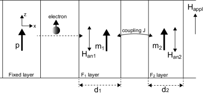
Let us first derive the Fokker-Planck equation for the synthetic free layer. The system we consider is schematically shown in Fig. 1. The two ferromagnetic layers, F₁ and F₂, consist of a synthetic free layer with the coupling energy $-JS\mathbf{m}_{1}\cdot\mathbf{m}_{2}$. Here $\mathbf{m}_{k}=\mathbf{M}_{k}/M_{k}=(\sin\theta_{k}\cos\varphi_{k},\sin\theta_{k}\sin\varphi_{k},\cos\theta_{k})$ is the unit vector along the direction of the magnetization $\mathbf{M}_{k}$ of the F_k layer. $J$ and $S$ are the coupling energy per unit area and the cross-sectional area of the system, respectively. It should be noted that $J>0$ and $J<0$ correspond to the ferromagnetically coupled and antiferromagnetically coupled synthetic free layers, respectively. Although we consider the ferromagnetically coupled system below, our formalism is applicable to the antiferromagnetically coupled system by changing the sign of the coupling constant $J$. We assume the uniaxial anisotropy along the $z$ axis for both F₁ and F₂ layers, and the magnetizations $\mathbf{m}_{1}$ and $\mathbf{m}_{2}$ point to the positive $z$ direction in the initial states. We also assume that the external field $H_{\rm appl}$ is applied along the $z$ axis. Then, the total free energy $F$ of the F₁ and F₂ layers are given by

$$\begin{split}F=&-M_{1}H_{\rm appl}V_{1}\cos\theta_{1}-\frac{1}{2}M_{1}H_{\rm an1}V_{1}\cos^{2}\theta_{1}\\ &-M_{2}H_{\rm appl}V_{2}\cos\theta_{2}-\frac{1}{2}M_{2}H_{\rm an2}V_{2}\cos^{2}\theta_{2}\\ &+2\pi M_{1}^{2}V_{1}(\sin\theta_{1}\cos\varphi_{1})^{2}+2\pi M_{2}^{2}V_{2}(\sin\theta_{2}\cos\varphi_{2})^{2}\\ &-JS\left[\sin\theta_{1}\sin\theta_{2}\cos(\varphi_{1}-\varphi_{2})+\cos\theta_{1}\cos\theta_{2}\right],\end{split}$$ (1)

where $H_{{\rm an}k}$, $V_{k}=Sd_{k}$ and $d_{k}$ are the uni-axial anisotropy field, the volume and the thickness of the F_k layer, respectively. The fifth and sixth terms in Eq. (1) represent the magnetic energy due to the demagnetization field. We assume that $|H_{\rm appl}|<H_{{\rm an}k}$ to guarantee at least two local minima of the free energy. When $H_{Jk}\ll H_{{\rm an}k}$, the states $(\mathbf{m}_{1},\mathbf{m}_{2})=(\mathbf{e}_{z},\mathbf{e}_{z})$, $(\mathbf{e}_{z},-\mathbf{e}_{z})$, $(-\mathbf{e}_{z},\mathbf{e}_{z})$, and $(-\mathbf{e}_{z},-\mathbf{e}_{z})$ correspond to the energy minima, where $H_{Jk}=J/(M_{k}d_{k})$. On the other hand, when $H_{Jk}\gg H_{{\rm an}k}$, the states $(\mathbf{m}_{1},\mathbf{m}_{2})=(\mathbf{e}_{z},\mathbf{e}_{z})$ and $(-\mathbf{e}_{z},-\mathbf{e}_{z})$ correspond to the energy minima.

The purpose of this paper is to investigate the switching rate of the magnetizations $\mathbf{m}_{1}$ and $\mathbf{m}_{2}$ from $\mathbf{m}_{1},\mathbf{m}_{2}=+\mathbf{e}_{z}$ to $\mathbf{m}_{1},\mathbf{m}_{2}=-\mathbf{e}_{z}$. Following Brown Jr (1963), we use the Fokker-Planck equation approach to calculate the switching probability per unit time, where the Fokker-Planck equation is derived from the equations of the motion of the magnetizations.

We assume that the dynamics of the magnetizations of the F₁ and F₂ layers are described by the Landau-Lifshitz-Gilbert (LLG) equations. In general, the spin transfer torque acting on $\mathbf{m}_{1}$ arises from the spin currents injected from the fixed layer and the F₂ layer. However, in a conventional synthetic free layer, the spacer layer between the F₁ and F₂ layers consists of Ru, whose spin diffusion length is comparable to its thickness com (a); thus, the spin current injected from the F₂ layer is negligible com (b). Then, the LLG equation of $\mathbf{m}_{1}$ is given by

$$\begin{split}\frac{{\rm d}\mathbf{m}_{1}}{{\rm d}t}=&-\gamma_{1}\mathbf{m}_{1}\times\mathbf{H}_{1}+\gamma_{1}a_{J}\mathbf{m}_{1}\times(\mathbf{p}\times\mathbf{m}_{1})\\ &-\gamma_{1}\mathbf{m}_{1}\times\mathbf{h}_{1}+\alpha_{1}\mathbf{m}_{1}\times\frac{{\rm d}\mathbf{m}_{1}}{{\rm d}t}.\end{split}$$ (2)

Similarly, the spin current injected from the F₁ layer into the F₂ layer is also negligible, and the LLG equation of $\mathbf{m}_{2}$ is given by

$$\begin{split}\frac{{\rm d}\mathbf{m}_{2}}{{\rm d}t}=&-\gamma_{2}\mathbf{m}_{2}\times\mathbf{H}_{2}-\gamma_{2}\mathbf{m}_{2}\times\mathbf{h}_{2}+\alpha_{2}\mathbf{m}_{2}\times\frac{{\rm d}\mathbf{m}_{2}}{{\rm d}t},\end{split}$$ (3)

where $\gamma_{k}$ and $\alpha_{k}$ are the gyromagnetic ratio and the Gilbert damping constant of the F_k layer, respectively. The magnetic field $\mathbf{H}_{k}$ acting on the magnetization $\mathbf{m}_{k}$ is defined by $\mathbf{H}_{k}=-(M_{k}V_{k})^{-1}\partial F/\partial\mathbf{m}_{k}$. $\mathbf{h}_{k}$ represents the random field on the F_k layer whose Cartesian components $h_{ki}$ ($i=x,y,z$) satisfy

$$\langle h_{ki}(t)h_{k^{\prime}j}(t^{\prime})\rangle=\frac{2k_{\rm B}T\alpha_{k}}{\gamma_{k}M_{k}V_{k}}\delta_{kk^{\prime}}\delta_{ij}\delta(t-t^{\prime}),$$ (4)

where $\langle\cdots\rangle$ means the ensemble average. Here we assume no correlation between the random fields acting on the F₁ and F₂ layers. The $a_{J}=\hbar\eta I/(2eM_{1}V_{1})$ term in Eq. (2) represents the spin transfer torque due to the injection of the spin current from the fixed layer. Here $I$ is the electric current flowing along the $x$ axis. The positive electric current corresponds to the electron flow along the $-x$ direction. $\eta$ is the spin polarization of the electric current which characterizes the strength of the spin transfer torque. The explicit form of $\eta$ depends on the theoretical model Slonczewski (1996); Brataas et al. (2001); Zhang et al. (2002), and, in general, depends on $\theta_{1}$. However, for simplicity, we assume that $\eta$ is constant (the dependence of $\eta$ on $\theta_{1}$ can be taken into account by replacing $a_{J}\cos\theta_{1}$ in Eq. (6) with $\int{\rm d}\cos\theta_{1}a_{J}$). $\mathbf{p}$ is the unit vector along the direction of the magnetization of the fixed layer.

From the LLG equations (2) and (3), we obtain the Fokker-Planck equation for the probability distribution of the directions of the magnetizations, $W(\mathbf{m}_{1},\mathbf{m}_{2})$, which is given by Jr (1963)

$$\begin{split}\frac{\partial W}{\partial t}&=\frac{\gamma_{1}}{M_{1}V_{1}}\frac{1}{\sin\theta_{1}}\frac{\partial}{\partial\theta_{1}}\\ &\ \ \ \ \ \left[\sin\theta_{1}\left\{\left(\alpha_{1}\frac{\partial F}{\partial\theta_{1}}+\frac{1}{\sin\theta_{1}}\frac{\partial F}{\partial\varphi_{1}}+a_{J}M_{1}V_{1}\sin\theta_{1}\right)W\right.\right.\\ &\ \ \ \ \ \ \ \ \ \ \ \ \ \ \ \ \ \ \ \ \ \ \ \ +\left.\left.\alpha_{1}k_{\rm B}T\frac{\partial W}{\partial\theta_{1}}\right\}\right]\\ &+\frac{\gamma_{1}}{M_{1}V_{1}}\frac{1}{\sin\theta_{1}}\frac{\partial}{\partial\varphi_{1}}\\ &\ \ \ \ \ \left[\left(\frac{\alpha_{1}}{\sin\theta_{1}}\frac{\partial F}{\partial\varphi_{1}}-\frac{\partial F}{\partial\theta_{1}}\right)W+\frac{\alpha_{1}k_{\rm B}T}{\sin\theta_{1}}\frac{\partial W}{\partial\varphi_{1}}\right]\\ &+\frac{\gamma_{2}}{M_{2}V_{2}}\frac{1}{\sin\theta_{2}}\frac{\partial}{\partial\theta_{2}}\\ &\ \ \ \ \ \left[\sin\theta_{2}\left\{\left(\alpha_{2}\frac{\partial F}{\partial\theta_{2}}+\frac{1}{\sin\theta_{2}}\frac{\partial F}{\partial\varphi_{2}}\right)W+\alpha_{2}k_{\rm B}T\frac{\partial W}{\partial\theta_{2}}\right\}\right]\\ &+\frac{\gamma_{2}}{M_{2}V_{2}}\frac{1}{\sin\theta_{2}}\frac{\partial}{\partial\varphi_{2}}\\ &\ \ \ \ \ \left[\left(\frac{\alpha_{2}}{\sin\theta_{2}}\frac{\partial F}{\partial\varphi_{2}}-\frac{\partial F}{\partial\theta_{2}}\right)W+\frac{\alpha_{2}k_{\rm B}T}{\sin\theta_{2}}\frac{\partial W}{\partial\varphi_{2}}\right]\ .\end{split}$$ (5)

Here we approximate that $1+\alpha_{k}^{2}\simeq 1$ by assuming that $\alpha_{k}\ll 1$ Oogane et al. (2006). We also neglect the term proportional to $\alpha a_{J}$ by assuming that $|a_{J}|<|\mathbf{H}_{k}|$, which is valid in the thermally assisted switching region.

As shown by Brown Jr (1963), the switching rate of the single ferromagnetic layer without spin transfer torque can be derived by using the steady-state solution of the Fokker-Planck equation and the continuity equation of the particles of an ensemble [see Sec. 4. C in Ref. Jr (1963)]. In the case of two ferromagnetic layers, as considered in this paper, the switching is described by the particle flow in $(\theta_{1},\varphi_{1},\theta_{2},\varphi_{2})$ four-dimensional phase space, and, in general, it is very difficult to obtain an analytical expression of the switching rate because the particle flow in the phase space is very complicated. To simplify the problem, we use the following two approximations.

Figure 2: The dependences of the effective potential $\mathscr{F}(\theta_{1},\theta_{2})$ on $\theta_{1}$ and $\theta_{2}$ for (a) the weak coupling limit and (b) the strong coupling limit. The values of the parameters are written in Secs. III and IV. The white arrows indicate the most probable paths of the switchings $\mathbf{m}_{1},\mathbf{m}_{2}=+\mathbf{e}_{z}\to-\mathbf{e}_{z}$.

First, we assume that the magnetization rotates in the $yz$ plane during the switching. Since the deviation of the magnetization $\mathbf{m}_{k}$ from the $yz$ plane increases the magnetic energy due to the demagnetization field, it is reasonable to assume that the most probable reversal process is the magnetization reversal in the $yz$ plane. In this limit, the demagnetization field plays no role on the calculation of the switching probability. By fixing the values of $\varphi_{1}$ and $\varphi_{2}$ to $\pi/2$ or $3\pi/2$, the steady-state solution of the Fokker-Planck equation (5) is given by $W_{0}\propto\exp[-\mathscr{F}/(k_{\rm B}T)]$, where the effective free energy $\mathscr{F}$ is given by

$$\mathscr{F}=F-\frac{a_{J}M_{1}V_{1}}{\alpha_{1}}\cos\theta_{1}.$$ (6)

The switching probability is calculated by using $W_{0}\propto\exp[-\mathscr{F}/(k_{\rm B}T)]$.

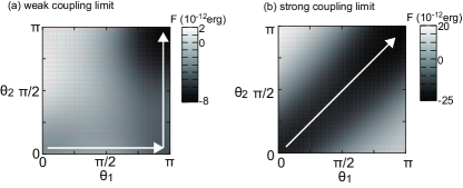
The second approximation is that we consider the switching for the weak and strong coupling limits, where the weak (strong) coupling means that the magnitude of the coupling energy of the F₁ and F₂ layers, $|-JS\mathbf{m}_{1}\cdot\mathbf{m}_{2}|$, is much smaller (larger) than the uniaxial anisotropy energy $M_{k}H_{{\rm an}k}V_{k}/2$. In other words, the weak (strong) coupling limit corresponds to $H_{{\rm an}k}\gg(\ll)H_{Jk}$. The weak and strong coupling limit can be realized by changing the thickness of the nonmagnetic layer $d_{\rm N}$ between F₁ and F₂ layers because the magnitude of the coupling constant $J$ strongly depends on $d_{\rm N}$ [see, for example, Fig. 2 in Ref. Hayakawa et al. (2008) or Fig. 1 (c) in Ref. Yakata et al. (2010)], and varies from $H_{J}\sim 1\times 10^{3}$ Oe to $1$ Oe or less. Figures 2 (a) and (b) show the dependences of $\mathscr{F}$ on $(\theta_{1},\theta_{2})$ for the weak and the strong coupling limit, respectively, where the white arrows indicate the most probable paths of the switching (the values of the parameters are written in Secs. III and IV with $a_{J}/a_{\rm c1}=0.5$). In the weak coupling limit, the magnetization reversal is divided into two steps: First $\mathbf{m}_{1}$ reverses its direction from $\mathbf{m}_{1}=+\mathbf{e}_{z}$ to $\mathbf{m}_{2}=-\mathbf{e}_{z}$ by the thermally assisted spin transfer torque effect while the direction of $\mathbf{m}_{2}$ is fixed to $\mathbf{m}_{2}=+\mathbf{e}_{z}$, and second, $\mathbf{m}_{2}$ reverses its direction by the thermal effect and the coupling with the F₁ layer while $\mathbf{m}_{1}$ is fixed to $\mathbf{m}_{1}=-\mathbf{e}_{z}$. On the other hand, in the strong coupling limit, $\mathbf{m}_{1}$ and $\mathbf{m}_{2}$ reverse their directions simultaneously.

By using the above two approximations, the calculation of the switching rate is reduced to a one-dimensional problem. For the weak coupling limit, first we calculate the particle flow in $\theta_{1}$ space, and second, we calculate the particle flow in $\theta_{2}$ space. On the other hand, for the strong coupling limit, we calculate the particle flow along the direction of $\theta_{1}=\theta_{2}$. For such one dimensional problems, the calculation method developed by Brown Jr (1963) is applicable to obtain the switching rate with some revisions. In Secs. III and IV, we show the switching probabilities for the weak and strong coupling limit, respectively.

At the end of this section, we give a brief comment on the first approximation. The influence of the first approximation is that the critical current density estimated in our calculation, $I_{\rm c}\propto(H_{\rm appl}+H_{\rm an})$, does not include the effect of the demagnetization field $4\pi M$ [see Eqs. (15), (16), (22) and (23)] while the critical current density estimated by the LLG equation includes the demagnetization field, that is, $I_{\rm c}\propto(H_{\rm appl}+H_{\rm an}+2\pi M)$ [see, for example, Eq. (14) in Ref. Li and Zhang (2004)]. Since $4\pi M\gg|H_{\rm appl}|,H_{\rm an}$, the critical current density in our formula ($10^{5-6}$ A/cm²) is much smaller than the experimental values ($10^{6-7}$ A/cm²) Hayakawa et al. (2008); Yakata et al. (2009, 2010). One way to solve this discrepancy is as follows. Although we consider the in-plane magnetized system, it should be noted that our calculation is directly applicable to the perpendicularly magnetized system where the system has uni-axial symmetry and the switchings in the weak and strong coupling limits are described by only $\theta_{1}$ and $\theta_{2}$. Suzuki et al. Suzki et al. (2009) showed that the effect of the demagnetization field on the switching rate of the in-plane magnetized system can be taken into account by replacing $H_{\rm an}$ in the switching formula of the perpendicularly magnetized system by $H_{\rm an}+2\pi M$. By applying this replacement to our formula, our formula may be applicable to analyze the experiments quantitatively. The validity of this replacement requires the numerical calculation of the Fokker-Planck equation, and it is beyond the scope of this paper.

III Weak coupling limit

In this section, we derive the switching rate of the magnetizations for the weak coupling limit ($H_{{\rm an}k}\gg H_{Jk}$) [see also the Appendix]. With this limit, the magnetization reversal is divided into two steps, as mentioned in Sec. II. For convenience, we label the three regions around the potential minimum in the phase space, $(\theta_{1},\theta_{2})=(0,0),(\pi,0)$, and $(\pi,\pi)$, as regions 1, 2, and 3, respectively. The first step ($\mathbf{m}_{1}$ reverses from $+\mathbf{e}_{z}$ to $-\mathbf{e}_{z}$) corresponds to the transition of the particle from region 1 to region 2 while the second step ($\mathbf{m}_{2}$ reverses from $+\mathbf{e}_{z}$ to $-\mathbf{e}_{z}$) corresponds to the transition from region 2 to region 3.

The switching rate from region 1 to region 2 is obtained as follows Jr (1963). In regions 1 and 2, the distribution $W(\theta_{1},\theta_{2})$ is given by $W_{1}\exp[-\{\mathscr{F}(\theta_{1},0)-\mathscr{F}(0,0)\}/(k_{\rm B}T)]$ and $W_{2}\exp[-\{\mathscr{F}(\theta_{1},0)-\mathscr{F}(\pi,0)\}/(k_{\rm B}T)]$, respectively, where $W_{1}=W(0,0)$ and $W_{2}=W(\pi,0)$. The numbers of particles in region 1, $n_{1}$, is obtained by integrating $W(\theta_{1},0)$ over $[0,\theta_{\rm m1}]$, where $\theta_{\rm m1}=\cos^{-1}[-(H_{\rm appl}+H_{J1}+a_{J}/\alpha_{1})/H_{\rm an1}]$ gives the local maximum of the effective potential $\mathscr{F}(\theta_{1},0)$. The explicit form of $n_{1}$ is given by $n_{1}=2W_{1}{\rm e}^{\mathscr{F}(0,0)/(k_{\rm B}T)}I_{1}$, where factor 2 arises from the fact that we restrict the particle flow in the $yz$ plane; that is, $\varphi_{1}=\pi/2$ or $3\pi/2$ (in the anisotropic system considered by Brown Jr (1963), the numerical factor is $2\pi$, not $2$, as shown in Eq. (4.26) of Ref. Jr (1963)). The integral $I_{1}=\int_{0}^{\theta_{\rm m1}}{\rm d}\theta_{1}\sin\theta_{1}\exp[-\mathscr{F}(\theta_{1},0)/(k_{\rm B}T)]$ can be approximated to Jr (1963)

$$\begin{split}I_{1}&\simeq{\rm e}^{-\mathscr{F}(0,0)/(k_{\rm B}T)}\int_{0}^{\infty}{\rm d}\theta_{1}\theta_{1}\exp\left[-\frac{1}{2k_{\rm B}T}\frac{\partial^{2}\mathscr{F}(\theta_{1},0)}{\partial\theta_{1}^{2}}\theta_{1}^{2}\right]\\ &={\rm e}^{-\mathscr{F}(0,0)/(k_{\rm B}T)}\frac{k_{\rm B}T}{\partial^{2}\mathscr{F}(0,0)/\partial\theta_{1}^{2}}.\end{split}$$ (7)

The numbers of particle in region 2, $n_{2}=2W_{2}{\rm e}^{\mathscr{F}(\pi,0)/(k_{\rm B}T)}I_{2}$, is obtained in a similar way by replacing the factors $\mathscr{F}(0,0)$ and $\partial^{2}\mathscr{F}(0,0)/\partial\theta_{1}^{2}$ to $\mathscr{F}(\pi,0)$ and $\partial^{2}\mathscr{F}(\pi,0)/\partial\theta_{1}^{2}$, respectively. Next, we consider the particle flow from region 1 to region 2, $I_{1\to 2}$. From the Fokker-Planck equation (5), the particle flow along the $\theta_{1}$-axis, $J_{\theta_{1}}$, which satisfies $I_{1\to 2}=2\sin\theta_{1}J_{\theta_{1}}$, is identified as

$$J_{\theta_{1}}=-\frac{\alpha_{1}\gamma_{1}}{M_{1}V_{1}}\left[\left(\frac{\partial F}{\partial\theta_{1}}+\frac{a_{J}M_{1}V_{1}}{\alpha_{1}}\sin\theta_{1}\right)W+k_{\rm B}T\frac{\partial W}{\partial\theta_{1}}\right].$$ (8)

By multiplying ${\rm e}^{\mathscr{F}(\theta_{1},0)/(k_{\rm B}T)}$ to $I_{1\to 2}/(2\sin\theta_{1})=J_{\theta_{1}}$ and integrating it over $[0,\pi]$, we find that $[(n_{2}/I_{2})-(n_{1}/I_{1})]/2=-[M_{1}V_{1}/(2\alpha_{1}\gamma_{1}k_{\rm B}T)]I_{1\to 2}I_{\rm m1}$, where the integral $I_{\rm m1}=\int_{0}^{\pi}{\rm d}\theta_{1}{\rm e}^{\mathscr{F}(\theta_{1},0)/(k_{\rm B}T)}/\sin\theta_{1}$ can be approximated to Jr (1963)

$$\begin{split}I_{\rm m1}&\simeq\frac{e^{\mathscr{F}(\theta_{\rm m1},0)/(k_{\rm B}T)}}{\sin\theta_{\rm m1}}\\ &\ \ \ \ \ \times\int_{-\infty}^{\infty}{\rm d}\theta_{1}\exp\left[\frac{(\theta_{1}-\theta_{\rm m1})^{2}}{2k_{\rm B}T}\frac{\partial^{2}\mathscr{F}(\theta_{\rm m1},0)}{\partial\theta_{1}^{2}}\right]\\ &=\sqrt{-\frac{2\pi k_{\rm B}T}{\partial^{2}\mathscr{F}(\theta_{\rm m1},0)/\partial\theta_{1}^{2}}}\frac{{\rm e}^{\mathscr{F}(\theta_{\rm m1},0)/(k_{\rm B}T)}}{\sin\theta_{\rm m1}}.\end{split}$$ (9)

The relation between the particle numbers in region 2 and 3, $n_{2}$ and $n_{3}$, and the particle flow from region 2 to region 3, $I_{2\to 3}$, is obtained in a similar way. Then, by using the continuity equations of the particle flow, $\dot{n}_{1}=-I_{1\to 2}$, $\dot{n}_{2}=I_{1\to 2}-I_{2\to 3}$, and $\dot{n}_{3}=I_{2\to 3}$, we find that the transitions of the magnetization directions among the three states, $(\theta_{1},\theta_{2})=(0,0),(\pi,0),(\pi,\pi)$, are described by the following differential equations:

$$\frac{{\rm d}}{{\rm d}t}\begin{pmatrix}n_{1}\\ n_{2}\\ n_{3}\end{pmatrix}=\begin{pmatrix}-\nu_{12}&\nu_{21}&0\\ \nu_{12}&-(\nu_{21}+\nu_{23})&\nu_{32}\\ 0&\nu_{23}&-\nu_{32}\end{pmatrix}\begin{pmatrix}n_{1}\\ n_{2}\\ n_{3}\end{pmatrix}.$$ (10)

The switching probability per unit time from the region $i$ to the region $j$ is given by $\nu_{ij}=f_{ij}\exp(-\Delta_{ij})$, where the attempt frequency $f_{ij}$ and the thermal stability $\Delta_{ij}$ are, respectively, given by

$$\begin{split}f_{12(21)}&=\left(\frac{\alpha_{1}\gamma_{1}k_{\rm B}T}{M_{1}V_{1}}\right)\frac{M_{1}H_{\rm an1}V_{1}}{k_{\rm B}T}\sqrt{\frac{M_{1}H_{\rm an1}V_{1}}{2\pi k_{\rm B}T}}\\ &\ \times\left(1+(-)\frac{H_{\rm appl}+H_{J1}}{H_{\rm an1}}\right)\left(1-\frac{I}{I_{\rm c1(2)}}\right)\\ &\ \times\left[1-\left(\frac{H_{\rm appl}+H_{J1}}{H_{\rm an1}}\right)^{2}\right]\left(1-\frac{I}{I_{\rm c1}}\right)\left(1-\frac{I}{I_{\rm c2}}\right),\end{split}$$ (11)

$$\begin{split}\Delta_{12(21)}&=\frac{M_{1}H_{\rm an1}V_{1}}{2k_{\rm B}T}\left(1+(-)\frac{H_{\rm appl}+H_{J1}}{H_{\rm an1}}\right)^{2}\\ &\ \times\left(1-\frac{I}{I_{\rm c1(2)}}\right)^{2},\end{split}$$ (12)

$$\begin{split}f_{23(32)}&=\left(\frac{\alpha_{2}\gamma_{2}k_{\rm B}T}{M_{2}V_{2}}\right)\frac{M_{2}H_{\rm an2}V_{2}}{k_{\rm B}T}\sqrt{\frac{M_{2}H_{\rm an2}V_{2}}{2\pi k_{\rm B}T}}\\ &\ \times\left(1+(-)\frac{H_{\rm appl}-H_{J2}}{H_{\rm an2}}\right)\\ &\ \times\left[1-\left(\frac{H_{\rm appl}-H_{J2}}{H_{\rm an2}}\right)^{2}\right],\end{split}$$ (13)

$$\Delta_{23(32)}=\frac{M_{2}H_{\rm an2}V_{2}}{2k_{\rm B}T}\left(1+(-)\frac{H_{\rm appl}-H_{J2}}{H_{\rm an2}}\right)^{2}.$$ (14)

Here $I/I_{\rm c1}=a_{J}/a_{\rm c1}$ and $I/I_{\rm c2}=a_{J}/a_{\rm c2}$. $a_{\rm c1}$ ($a_{\rm c2}$) is the critical spin-transfer torque field to induce the magnetization reversal from region 1 (2) to region 2 (1) at zero temperature, and their explicit forms are given by

$$a_{\rm c1}=-\alpha_{1}\left(H_{\rm appl}+H_{J1}+H_{\rm an1}\right),$$ (15)

$$a_{\rm c2}=\alpha_{1}\left(-H_{\rm appl}-H_{J1}+H_{\rm an1}\right),$$ (16)

respectively. Since $|H_{\rm appl}+H_{J1}|$ is assumed to be smaller than $H_{\rm an1}$, we find that $a_{\rm c1}<0$ and $a_{\rm c2}>0$. It should be noted that the description of the transition of the magnetization by Eq. (10) is valid for $|a_{J}|<|a_{{\rm c}k}|$ because if $|a_{J}|\gg|a_{\rm c1}|(|a_{\rm c2}|)$, the point $\mathbf{m}_{1}=+\mathbf{e}_{z}(-\mathbf{e}_{z})$ would be unstable, and then we could not discuss the thermally assisted transition. We also note that the switching probabilities of $\mathbf{m}_{2}$, $\nu_{23}$ and $\nu_{32}$, are reduced to those obtained by Brown Jr (1963) by omitting $H_{J2}$ where $\nu_{23}$ and $\nu_{32}$ are independent of the current $I$.

Figure 3: (a) Time evolution of $n_{1}(t)$, $n_{2}(t)$, and $n_{3}(t)$ with $I/I_{\rm c1}=0.7$ for the weak coupling limit. (b) The dependence of the switching rate $n_{3}(t)$ on the ratio $I/I_{\rm c1}$ for the weak coupling limit. For $I/I_{\rm c1}\geq 0.8$, the switching time is saturated. The horizontal axis is the logarithmic scale.

When $I$ is nearly $I_{\rm c1}$, we find that $\nu_{12}/\nu_{21}\sim\exp[M_{1}H_{\rm an1}V_{1}/(2k_{\rm B}T)]\gg 1$. Similarly, when $-H_{\rm appl}+H_{J2}>0$, we find that $\nu_{23}/\nu_{32}\sim\exp[2M_{2}(-H_{\rm appl}+H_{J2})V_{2}/(2k_{\rm B}T)]\gg 1$. Within these limits, the analytical solutions of Eq. (10) with the initial conditions $n_{1}(0)=1$, $n_{2}(0)=0$, and $n_{3}(0)=0$, are given by

$$n_{1}(t)={\rm e}^{-\nu_{12}t},$$ (17)

$$n_{2}(t)=-\frac{\nu_{12}}{\nu_{12}-\nu_{23}}\left({\rm e}^{-\nu_{12}t}-{\rm e}^{-\nu_{23}t}\right),$$ (18)

$$n_{3}(t)=1-\frac{\nu_{12}{\rm e}^{-\nu_{23}t}-\nu_{23}{\rm e}^{-\nu_{12}t}}{\nu_{12}-\nu_{23}}.$$ (19)

Equation (19) is the central result of this section: It completely describes the magnetization switching of the synthetic free layer within the weak coupling limit.

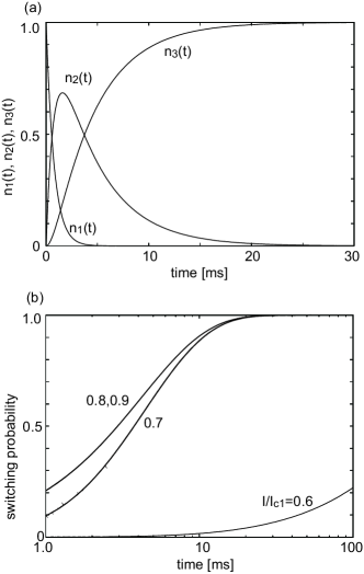
Figure 3 (a) shows a typical time evolution of $n_{1}(t)$, $n_{2}(t)$, and $n_{3}(t)$ for a synthetic free layer with $M=995$ emu/c.c., $H_{\rm an}=50$ Oe, $H_{\rm appl}=0$ Oe, $\alpha=0.007$, $\gamma=1.732\times 10^{7}$ Hz/Oe, $d=2$ nm, $S=\pi\times 70\times 160$ nm², and $T=300$ K (for simplicity, we assume that F₁=F₂) Yakata et al. (2009, 2010); com (c). The current is taken to be $I/I_{\rm c1}=0.7$. The coupling constant is assumed to be $J=5.0\times 10^{-3}$ erg/cm², which corresponds to $H_{J}=25$ Oe. From Eqs. (17), (18) and (19), one can easily see that the time evolution shown in Fig. 3 (a) is determined by two time scales, $\nu_{12}^{-1}$ and $\nu_{23}^{-1}$, which correspond to the switching rates of the F₁ and F₂ layers, respectively. Figure 3 (b) shows the dependence of the switching rate $n_{3}(t)$ on the ratio $I/I_{\rm c1}$. For the currents $|I|\geq 0.7|I_{\rm c1}|$, the switching times are on the same order ($10$ ms for our parameters), and for the large currents $|I|\geq 0.8|I_{\rm c1}|$, the switching times are saturated. This is because the current determines the switching time of the F₁ layer only, and for a large current, the total switching time of $\mathbf{m}_{1}$ and $\mathbf{m}_{2}$ is mainly determined by the switching time of $\mathbf{m}_{2}$, which is independent of the current. We can verify the saturation of the switching time from Eq. (19), where $\nu_{12}$ becomes much larger than $\nu_{23}$ as $I$ approaches $I_{\rm c1}$ and then, $n_{3}(t)\simeq 1-{\rm e}^{-\nu_{23}t}$, which is independent of the current $I$. On the other hand, in the low current region $|I|\ll|I_{\rm c1}|$, $\nu_{12}$ becomes comparable or smaller than $\nu_{23}$, which leads to $n_{3}(t)\simeq 1-{\rm e}^{-\nu_{12}t}$. Then the switching time strongly depends on the current value because the switching time of $\mathbf{m}_{1}$ becomes important to the total switching time. For example, the switching time for $I/I_{\rm c1}=0.6$ is longer than 100 ms, as shown in Fig. 3 (b).

The dependence of the switching time on the coupling constant $J$ is as follow. By increasing the magnitude of $H_{J}$, the switching time rapidly decreases because of the fast reversal of the magentization of the F₂ layer. For example, for $H_{J}=40$ Oe with $I/I_{\rm c}=0.9$, the switching time is on the order of $10^{-2}$ ms, which is three orders of magnitude faster than that for $H_{J}=25$ Oe. On the other hand, by decreasing the magnitude of $H_{J}$, only the magnetization of the F₁ layer reverses its direction while the magnetization of the F₂ layer remains $\mathbf{m}_{2}=+\mathbf{e}_{z}$. For example, for $H_{J}=5$ Oe with $I/I_{\rm c}=0.9$, the switching time of the F₁ layer is on the order of $10^{-2}$ ms while the switching rate of the F₂ layer, $n_{3}$, is approximately zero ($n_{3}\sim 10^{-9}$). Since the switching of the F₂ layer is induced by the coupling with the F₁ layer, it is required to increase the magnitude of the coupling constant $J$ for the fast switching by using a thin nonmagnetic spacer, although the increase of the coupling constant leads to the increase of the magnitude of the critical current density.

Figure 4: The dependence of the switching rate $n_{2}(t)$ on the ratio $I/I_{\rm c1}$ for the strong coupling limit. The horizontal axis is the logarithmic scale.

IV Strong coupling limit

In this section, we derive the switching rate of the magnetizations for the strong coupling limit ($H_{{\rm an}k}\ll H_{Jk}$). For this limit, instead of $(\theta_{1},\theta_{2})$ phase space, it is convenient to describe the particle flow in $(\Psi,\psi)$ phase space, where $\Psi=(\theta_{1}+\theta_{2})/2$ and $\psi=\theta_{1}-\theta_{2}$. Since $\mathbf{m}_{1}$ and $\mathbf{m}_{2}$ reverse their directions simultaneously, the reversal is described by the particle flow along the $\Psi$-axis with $\psi=0$. For convenience, we label the two regions around the potential minimum in the phase space, $(\Psi,\psi)=(0,0)$ and $(\pi,0)$, as regions 1 and 2, respectively. The continuity equation of the particle in the regions 1 and 2 is obtained in a way similar to that described in Sec. III and is expressed as $\dot{n}_{1}=-\dot{n}_{2}=-\nu_{12}n_{1}+\nu_{21}n_{2}$. The switching probability $\nu_{ij}=f_{ij}\exp(-\Delta_{ij})$ is given by

$$\begin{split}f_{12(21)}&=\frac{k_{\rm B}T}{2}\left(\frac{\alpha_{1}\gamma_{1}}{M_{1}V_{1}}+\frac{\alpha_{2}\gamma_{2}}{M_{2}V_{2}}\right)\frac{M_{1}H_{\rm an1}V_{1}+M_{2}H_{\rm an2}V_{2}}{k_{\rm B}T}\\ &\ \times\sqrt{\frac{M_{1}H_{\rm an1}V_{1}+M_{2}H_{\rm an2}V_{2}}{2\pi k_{\rm B}T}}\\ &\ \times\left(1+(-)\frac{M_{1}H_{\rm appl}V_{1}+M_{2}H_{\rm appl}V_{2}}{M_{1}H_{\rm an1}V_{1}+M_{2}H_{\rm an2}V_{2}}\right)\left(1-\frac{I}{I_{\rm c1(2)}}\right)\\ &\ \times\left[1-\left(\frac{M_{1}H_{\rm appl}V_{1}+M_{2}H_{\rm appl}V_{2}}{M_{1}H_{\rm an1}V_{1}+M_{2}H_{\rm an2}V_{2}}\right)^{2}\right]\\ &\ \times\left(1-\frac{I}{I_{\rm c1}}\right)\left(1-\frac{I}{I_{\rm c2}}\right),\end{split}$$ (20)

$$\begin{split}\Delta_{12(21)}&=\frac{M_{1}H_{\rm an1}V_{1}+M_{2}H_{\rm an2}V_{2}}{2k_{\rm B}T}\\ &\ \times\left(1+(-)\frac{M_{1}H_{\rm appl}V_{1}+M_{2}H_{\rm appl}V_{2}}{M_{1}H_{\rm an1}V_{1}+M_{2}H_{\rm an2}V_{2}}\right)^{2}\\ &\ \times\left(1-\frac{I}{I_{\rm c1(2)}}\right)^{2},\end{split}$$ (21)

where $I/I_{\rm c1}=a_{J}/a_{\rm c1}$ and $I/I_{\rm c2}=a_{J}/a_{\rm c2}$, and the critical spin-transfer torque fields in the strong coupling limit $a_{{\rm c}k}$ are given by

$$a_{\rm c1}=-\alpha_{1}\left[H_{\rm appl}+H_{\rm an1}+\frac{M_{2}V_{2}}{M_{1}V_{1}}\left(H_{\rm appl}+H_{\rm an2}\right)\right],$$ (22)

$$a_{\rm c2}=\alpha_{1}\left[-H_{\rm appl}+H_{\rm an1}+\frac{M_{2}V_{2}}{M_{1}V_{1}}\left(-H_{\rm appl}+H_{\rm an2}\right)\right],$$ (23)

respectively. The analytical solutions of the transition equations, $\dot{n}_{1}=-\dot{n}_{2}=-\nu_{12}n_{1}+\nu_{21}n_{2}$, with the initial conditions $n_{1}(0)=1$ and $n_{2}(0)=0$ are given by

$$n_{1}(t)=\frac{\nu_{21}}{\nu_{12}+\nu_{21}}+\frac{\nu_{12}}{\nu_{12}+\nu_{21}}{\rm e}^{-(\nu_{12}+\nu_{21})t},$$ (24)

$$n_{2}(t)=\frac{\nu_{12}}{\nu_{12}+\nu_{21}}-\frac{\nu_{12}}{\nu_{12}+\nu_{21}}{\rm e}^{-(\nu_{12}+\nu_{21})t}.$$ (25)

When $I$ is nearly $I_{\rm c1}$, $\nu_{12}/\nu_{21}\sim\exp[(M_{1}H_{\rm an1}V_{1}+M_{2}H_{\rm an2}V_{2})/(2k_{\rm B}T)]\gg 1$. For this limit, Eqs. (24) and (25) are reduced to

$$n_{1}(t)\simeq{\rm e}^{-\nu_{12}t},$$ (26)

$$n_{2}(t)\simeq 1-{\rm e}^{-\nu_{12}t}.$$ (27)

Equation (27) is the central result of this section: It completely describes the magnetization switching of the synthetic free layer within the strong coupling limit.

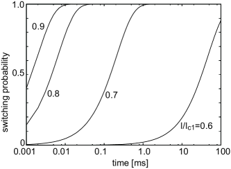
For the strong coupling limit, the switching time strongly depends on the current $I$ for all current region. Figure 4 shows the dependence of $n_{2}(t)$ on the ratio $I/I_{\rm c1}$, where the parameters used are same as those in Fig. 3 except $J$. The coupling constant $J$ is assumed to be $5.0\times 10^{-2}$ erg/cm^-2, which corresponds to $H_{J}=250$ Oe. The orders of the switching times are $10^{-2}$ ms for $I/I_{\rm c1}=0.8,0.9$, $1$ ms for $I/I_{\rm c1}=0.7$, and more than $100$ ms for $I/I_{\rm c1}\leq 0.6$ in our parameter region, as shown in Fig. 4. Such strong dependence of the switching time on the current arises from the thermal stability $\Delta_{12}$, which is proportional to $(1-I/I_{\rm c1})^{2}$, as shown in Eq. (21).

V Relation to other works

In this section, we compare the results obtained in the previous sections to the other works Hayakawa et al. (2008); Yakata et al. (2009, 2010); Koch et al. (2004). The topics discussed here are (1) the comparison of the switching time of the ferromagnetically (F) and the anti-ferromagnetically (AF) coupled synthetic free layers, and (2) the comparison of the dependence of the thermal stability to that obtained by Koch et al. Koch et al. (2004).

Figure 5: (a), (b): The schematic views of the alignments of the magnetizations $\mathbf{m}_{1}$ and $\mathbf{m}_{2}$ of (a) ferromagnetically (F) coupled and (b) anti-ferromagnetically (AF) coupled synthetic free layers after $\mathbf{m}_{1}$ reverses its direction from the initial state ($\mathbf{m}_{1}=+\mathbf{e}_{z}$) to $\mathbf{m}_{1}=-\mathbf{e}_{z}$. The directions of the applied field $H_{\rm appl}$ (assumed to be positive) and the coupling field $H_{J2}$ are also denoted. (c), (d): The time evolution of $n_{3}(t)$ of the F-coupled ($n_{3}^{({\rm F})}(t)$) and the AF-coupled ($n_{3}^{({\rm AF})}(t)$) synthetic free layer with (c) $H_{\rm appl}=+5$ Oe and (d) $H_{\rm appl}=-5$ Oe. The value of the current is taken to be $I/I_{\rm c1}=0.7$.

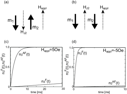
First, we discuss the switching times of the F and the AF-coupled synthetic free layers. The difference in the switching times of these two kinds of synthetic free layer appears in the weak coupling limit with finite $H_{\rm appl}$. In this case, the switching time of the F-coupled synthetic free layer is characterized by Eqs. (12) and (14). For the AF-coupled synthetic free layer, the factor $+(-)(H_{\rm appl}-H_{J2})/H_{\rm an2}$ in Eq. (14) is replaced by $-(+)(H_{\rm appl}+H_{J2})/H_{\rm an2}$ while Eq. (12) remains the same. This replacement is due to the fact that after $\mathbf{m}_{1}$ reverses its direction from $+\mathbf{e}_{z}$ to $-\mathbf{e}_{z}$, the sum of the applied field $H_{\rm appl}$ and the coupling field $H_{J2}$ acting on $\mathbf{m}_{2}$ is $H_{\rm appl}-H_{J2}$ for the F-coupled synthetic free layer while it is $H_{\rm appl}+H_{J2}$ for the AF-coupled synthetic free layer, as schematically shown in Figs. 5 (a) and (b), and leads to the difference in the switching times of the F-coupled and the AF-coupled synthetic layers.

The important point is that the fast switching is achieved by choosing the appropriate direction of $H_{\rm appl}$. Figures 5 (c) and (d) show the time evolutions of $n_{3}(t)$ (Eq. (19)) for the F-coupled ($n_{3}^{({\rm F})}$) and the AF-coupled ($n_{3}^{({\rm AF})}$) synthetic free layers with (c) $H_{\rm appl}=+5$ Oe and (d) $H_{\rm appl}=-5$ Oe. The current is taken to be $I/I_{\rm c1}=0.7$. The switching time of the AF (F) coupled synthetic free layer is faster compared to that of the F (AF) coupled synthetic free layer for $H_{\rm appl}>0(<0)$ because both $H_{\rm appl}$ and $H_{J2}$ assist the reversal of $\mathbf{m}_{2}$. On the other hand, by changing the direction (sign) of $H_{\rm appl}$, the switching time increases significantly because of the exponential dependence of the switching time ($\sim 1/\nu$) on $\Delta\propto[1-(H_{\rm appl}\pm H_{J})/H_{\rm an}]^{2}$. The difference between $n_{3}^{({\rm AF})}$ with $H_{\rm appl}>0$ and $n_{3}^{({\rm F})}$ with $H_{\rm appl}<0$ arises from the dependence of the switching time of $\mathbf{m}_{1}$ on the direction of $H_{\rm appl}$, and becomes negligible as $I$ approaches $I_{\rm c1}$ because the total switching time is mainly determined by that of $\mathbf{m}_{2}$ within the limit of $I/I_{\rm c1}\to 1$, as mentioned in Sec. III. For the strong coupling limit, the switching times of the F-coupled and the AF-coupled synthetic free layers are the same because the coupling energy is constant during the switching in this limit, and the coupling field $H_{J}$ plays no role on the switching.

Second, we discuss the dependence of the thermal stability $\Delta$ on the current $I$. As shown in Eqs. (12) and (21), our calculations show that $\Delta\propto\Delta_{0}(1-I/I_{\rm c})^{2}$. It should be noted that our formula is applicable to the single free layer by omitting the coupling of the F₁ and the F₂ layers, and thus, even for the single free layer we find that $\Delta\propto\Delta_{0}(1-I/I_{\rm c})^{2}$. Recently, a similar result was obtained by Suzuki et al. Suzki et al. (2009) and Butler et al. com (c) for the perpendicularly magnetized single free layer. However, the formula of the switching rate with $\Delta\propto\Delta_{0}(1-I/I_{\rm c})$ first obtained by Koch et al. Koch et al. (2004) has been widely used to fit the experiments Hayakawa et al. (2008); Yakata et al. (2009, 2010).

The important point is that the difference of the exponent of $(1-I/I_{\rm c})$ leads to a significant underestimation of $\Delta_{0}$. Let us consider the fit of the experimental results of the switching rate with the formula $P=1-\exp\{-f_{0}t\exp[-\Delta_{0}(1-I/I_{\rm c})^{n}]\}$, where for simplicity we assume that the attempt frequency $f_{ij}$ is constant $f_{0}$. When $I/I_{\rm c}=0.5$, the thermal stability $\Delta_{0}$ estimated by our formula ($n=2$) is two times larger than that estimated by the conventional formula ($n=1$).

The difference between the exponent of $(1-I/I_{\rm c})$ in our calculation and that in the theory of Koch et al. Koch et al. (2004) arises from the steady-state solution of the Fokker-Planck equation of the free layer magnetization:

$$\begin{split}\frac{\partial W}{\partial t}=&\frac{\alpha\gamma}{MV}\frac{1}{\sin\theta}\frac{\partial}{\partial\theta}\\ &\ \ \left[\sin\theta\left\{\left(\frac{\partial F}{\partial\theta}+\frac{a_{J}MV}{\alpha}\sin\theta\right)W+k_{\rm B}T\frac{\partial W}{\partial\theta}\right\}\right].\end{split}$$ (28)

Koch et al. argued that the steady-state solution of of Eq. (28) is $W_{\rm Koch}\propto\exp\{-F[1+a_{J}/(\alpha H)]/(k_{\rm B}T)\}$, where $H=|\mathbf{H}|$ is the absolute value of the magnetic field acting on the free layer magnetization. However, when $H$ depends on $\mathbf{m}$, $W_{\rm Koch}$ is not a steady state solution of Eq. (28). In general, $H$ depends on $\mathbf{m}$ because of the presence of the uni-axial anisotropy field $\mathbf{H}_{\rm an}=H_{\rm an}m_{z}\mathbf{e}_{z}$, which guarantees two local minima of the free energy $F$. Thus, in the calculation of the switching rate, we should use $W_{0}\propto\exp\{-[1-(a_{J}MV\cos\theta)/(\alpha F)/(k_{\rm B}T)]\}$, which is the steady state solution of Eq. (28) as shown in Sec. II, instead of $W_{\rm Koch}$. The difference between $W_{0}$ and $W_{\rm Koch}$ leads to that of the exponent of $(1-I/I_{\rm c})$ in $\Delta$.

VI Conclusions

In conclusion, we studied the magnetization switching of the synthetic free layer theoretically by solving the Fokker-Planck equation. We obtained the analytical expression of the switching rate for the weak and the strong coupling limits, given by Eqs. (19) and (27). We found that the switching time within the weak coupling limit becomes saturated as the current $I$ approaches the critical current $I_{\rm c1}$. We compared the switching time of the ferromagnetically and the anti-ferromagnetically coupled synthetic free layers with a finite applied field, and find that fast switching is achieved by choosing the appropriate direction of the applied field. We also found that the dependence of the thermal stability on the current is $\Delta\propto\Delta_{0}(1-I/I_{\rm c})^{2}$, not $\Delta\propto\Delta_{0}(1-I/I_{\rm c})$ as argued by previous authors Koch et al. (2004), which leads to a significant underestimation of $\Delta_{0}$.

APPENDIX A: DETAILS OF THE CALCULATION IN SEC. III

In this appendix, we show the details of the derivation of Eq. (19) [see also Sec. 4 C in Ref. Jr (1963)]. First, let us consider the switching from region 1 to region 2. The number of the particle in region 1 is obtained by integrating $2W_{1}\exp[-\{\mathscr{F}(\theta_{1},0)-\mathscr{F}(0,0)\}/(k_{\rm B}T)]$ over $0\leq\theta_{\rm m1}\leq\theta_{\rm m1}$; that is,

$$n_{1}=2W_{1}{\rm e}^{\mathscr{F}(0,0)/(k_{\rm B}T)}\int_{0}^{\theta_{\rm m1}}{\rm d}\theta_{1}\sin\theta_{1}\exp\left[-\frac{\mathscr{F}(\theta_{1},0)}{k_{\rm B}T}\right].$$ (29)

It should be noted that the exponential term in the integral rapidly decreases by changing $\theta_{1}$ from 0 to $\theta_{\rm m1}$. Then, we replace $\mathscr{F}(\theta_{1},0)$ by its Taylor series about $\theta_{1}=0$, keep the terms up to the second order of $\theta_{1}$, and replace the upper limit of the integral by $\infty$. The first term of Taylor series, $\partial\mathscr{F}(0,0)/\partial\theta_{1}$, is zero because $\theta_{1}=0$ corresponds to the local minimum of $\mathscr{F}$. $\sin\theta_{1}$ is approximated to $\theta_{1}$. Then, we arrive Eq. (7). The numer of the particle in region 2, $n_{2}$, is obtained in a similar way; that is, $n_{2}=2W_{2}{\rm e}^{\mathscr{F}(\pi,0)/(k_{\rm B}T)}I_{2}$, where $I_{2}$ is given by

$$I_{2}={\rm e}^{-\mathscr{F}(\pi,0)/(k_{\rm B}T)}\frac{k_{\rm B}T}{\partial^{2}\mathscr{F}(\pi,0)/\partial\theta_{1}^{2}}.$$ (30)

The particle flow from region 1 to region 2, $I_{1\to 2}$, satisfies [see Eq. (8)]

$$\frac{\partial W}{\partial\theta_{1}}+\frac{1}{k_{\rm B}T}\frac{\partial\mathscr{F}}{\partial\theta_{1}}W=-\left(\frac{M_{1}V_{1}}{\alpha_{1}\gamma_{1}k_{\rm B}T}\right)\frac{I_{1\to 2}}{2\sin\theta_{1}}.$$ (31)

According to Brown Jr (1963), we assume that $I_{1\to 2}$ is independent of $\theta_{1}$. By multiplying ${\rm e}^{\mathscr{F}(\theta_{1},0)/(k_{\rm B}T)}$ to Eq. (31) and integrating it over $[0,\pi]$, the left hand side of Eq. (31) is reduced to

$$\begin{split}&\int_{0}^{\pi}{\rm d}\theta_{1}\frac{\partial}{\partial\theta_{1}}W{\rm e}^{\mathscr{F}(\theta_{1},0)/(k_{\rm B}T)}\\ &=W(\pi,0){\rm e}^{\mathscr{F}(\pi,0)/(k_{\rm B}T)}-W(0,0){\rm e}^{\mathscr{F}(0,0)/(k_{\rm B}T)}\\ &=\frac{1}{2}\left(\frac{n_{2}}{I_{2}}-\frac{n_{1}}{I_{1}}\right),\end{split}$$ (32)

where we use the definitions of $I_{1}$ and $I_{2}$, i.e., $n_{1}=2W_{1}{\rm e}^{\mathscr{F}(0,0)/(k_{\rm B}T)}I_{1}$ and $n_{2}=2W_{2}{\rm e}^{\mathscr{F}(\pi,0)/(k_{\rm B}T)}I_{2}$. On the other hand, by using Taylor series of $\mathscr{F}(\theta_{1},0)$ about $\theta_{1}=\theta_{\rm m1}$, the right hand side of Eq. (31) is approximated to $-[M_{1}V_{1}/(2\alpha_{1}\gamma_{1}k_{\rm B}T)]I_{1\to 2}I_{\rm m1}$, where $I_{\rm m1}$ is given by Eq. (9). Thus, we obtain

$$\frac{1}{2}\left(\frac{n_{2}}{I_{2}}-\frac{n_{1}}{I_{1}}\right)=-\frac{M_{1}V_{1}}{2\alpha_{1}\gamma_{1}k_{\rm B}T}I_{1\to 2}I_{\rm m1}.$$ (33)

Similarly, the number of the particles in regions 2 and 3, $n_{2}$ and $n_{3}$, and the particle flow from the region 2 to region 3, $I_{2\to 3}$, satisfy

$$\frac{1}{2}\left(\frac{n_{3}}{I_{3}^{\prime}}-\frac{n_{2}}{I_{2}^{\prime}}\right)=-\frac{M_{2}V_{2}}{2\alpha_{2}\gamma_{2}k_{\rm B}T}I_{2\to 3}I_{\rm m2},$$ (34)

where $I_{2}^{\prime}$, $I_{3}^{\prime}$, and $I_{\rm m2}$ are, respectively, given by

$$I_{2}^{\prime}={\rm e}^{-\mathscr{F}(\pi,0)/(k_{\rm B}T)}\frac{k_{\rm B}T}{\partial^{2}\mathscr{F}(\pi,0)/\partial\theta_{2}^{2}},$$ (35)

$$I_{3}^{\prime}={\rm e}^{-\mathscr{F}(\pi,\pi)/(k_{\rm B}T)}\frac{k_{\rm B}T}{\partial^{2}\mathscr{F}(\pi,\pi)/\partial\theta_{2}^{2}},$$ (36)

$$I_{\rm m2}=\sqrt{-\frac{2\pi k_{\rm B}T}{\partial^{2}\mathscr{F}(\pi,\theta_{\rm m2})/\partial\theta_{\rm 2}^{2}}}\frac{{\rm e}^{\mathscr{F}(\pi,\theta_{\rm m2})/(k_{\rm B}T)}}{\sin\theta_{\rm m2}},$$ (37)

where $\theta_{\rm m2}=\cos^{-1}[-(H_{\rm appl}-H_{J2})/H_{\rm an2}]$.

By using Eqs. (33), (34) and the continuity equations of the particle flows, $\dot{n}_{1}=-I_{1\to 2}$, $\dot{n}_{2}=I_{1\to 2}-I_{2\to 3}$, and $\dot{n}_{3}=I_{2\to 3}$, we obtain Eq. (10). The switching probabilities per unit time, $\nu_{ij}$, are given by

$$\nu_{12}=\left(\frac{\alpha_{1}\gamma_{1}k_{\rm B}T}{M_{1}V_{1}}\right)\frac{1}{I_{1}I_{\rm m1}},$$ (38)

$$\nu_{21}=\left(\frac{\alpha_{1}\gamma_{1}k_{\rm B}T}{M_{1}V_{1}}\right)\frac{1}{I_{2}I_{\rm m1}},$$ (39)

$$\nu_{23}=\left(\frac{\alpha_{2}\gamma_{2}k_{\rm B}T}{M_{2}V_{2}}\right)\frac{1}{I_{2}^{\prime}I_{\rm m2}},$$ (40)

$$\nu_{32}=\left(\frac{\alpha_{2}\gamma_{2}k_{\rm B}T}{M_{2}V_{2}}\right)\frac{1}{I_{3}^{\prime}I_{\rm m2}}.$$ (41)

The explicit forms of $\nu_{ij}$ are obtained by using $\mathscr{F}(\theta_{1},\theta_{2})$ and its derivative, and given by Eqs. (11)-(14).

By applying the negative current and magnetic field, which induce the magnetization reversal from $\mathbf{m}_{1},\mathbf{m}_{2}=+\mathbf{e}_{z}$ to $\mathbf{m}_{1},\mathbf{m}_{2}=-\mathbf{e}_{z}$, $\nu_{12}$ and $\nu_{23}$ become much larger than $\nu_{21}$ and $\nu_{32}$, respectively. Then, Eq. (10) can be approximated to $\dot{n}_{1}=-\nu_{12}n_{1}$, $\dot{n}_{2}=\nu_{12}n_{1}-\nu_{23}n_{2}$ and $\dot{n}_{3}=\nu_{23}n_{2}$. Then, the solutions of $n_{1}$, $n_{2}$, and $n_{3}$ with the initial conditions, $n_{1}(0)=1$, $n_{2}(0)=0$, and $n_{3}(0)=0$, are given by Eqs. (17)-(19).

References

- Slonczewski (1996) J. C. Slonczewski, J. Magn. Magn. Mater. 159, L1 (1996).
- Slonczewski (1989) J. C. Slonczewski, Phys. Rev. B 39, 6995 (1989).
- Berger (1996) L. Berger, Phys. Rev. B 54, 9353 (1996).
- Katine et al. (2000) J. A. Katine, F. J. Albert, R. A. Buhrman, E. B. Myers, and D. C. Ralph, Phys. Rev. Lett. 84, 3149 (2000).
- Kiselev et al. (2003) S. I. Kiselev, J. C. Sankey, I. N. Krivorotov, N. C. Emley, R. J. Schoelkopf, R. A. Buhrman, and D. C. Ralph, Nature 425, 380 (2003).
- Huai et al. (2004) Y. Huai, F. Albert, P. Nguyen, M. Pakala, and T. Valet, Appl. Phys. Lett. 84, 3118 (2004).
- Fuchs et al. (2004) G. D. Fuchs, N. C. Emley, I. N. Krivorotov, P. M. Braganca, E. M. Ryan, S. I. Kiselev, J. C. Sankey, D. C. Ralph, R. A. Buhrman, and J. A. Katine, Appl. Phys. Lett. 85, 1205 (2004).
- Hayakawa et al. (2008) J. Hayakawa, S. Ikeda, K. Miura, M. Yamanouchi, Y. M. Lee, R. Sasaki, M. Ichimura, K. Ito, T. Kawahara, R. Takemura, T. Meguro, F. Matsukura, H. Takahashi, H. Matsuoka, and H. Ohno, IEEE. Trans. Magn. 44, 1962 (2008).
- Yakata et al. (2009) S. Yakata, H. Kubota, T. Sugano, T. Seki, K. Yakushiji, A. Fukushima, S. Yuasa, and K. Ando, Appl. Phys. Lett. 95, 242504 (2009).
- Yakata et al. (2010) S. Yakata, H. Kubota, T. Seki, K. Yakushiji, A. Fukushima, S. Yuasa, and K. Ando, IEEE. Trans. Magn. 46, 2232 (2010).
- Koch et al. (2004) R. H. Koch, J. A. Katine, and J. Z. Sun, Phys. Rev. Lett. 92, 088302 (2004).
- Li and Zhang (2004) Z. Li and S. Zhang, Phys. Rev. B 69, 134416 (2004).
- Apalkov and Visscher (2005) D. M. Apalkov and P. B. Visscher, Phys. Rev. B 72, 180405 (2005).
- Jr (1963) W. F. B. Jr, Phys. Rev. 130, 1677 (1963).
- com (a) The spin transfer torque switching in the synthetic free layer is performed at room temperature using an Ru layer with a thickness of a few nm Hayakawa et al. (2008); Yakata et al. (2009, 2010). The spin diffusion length of Ru at 4.2 K is 14 nm Bass and W. P. Pratt (2007) and it would be much smaller at room temperature.
- com (b) Private communication with Hitoshi Kubota. It was experimentally shown that the critical current of the spin transfer torque switching in a CoFeB/Ru/CoFeB spin-valve is one order of magnitude larger than that in CoFeB/MgO/CoFeB MTJs (unpublished). This result means that the spin transfer torque arising between the free layers of the synthetic structure is negligible compared to that arising from the spin current injected from the fixed layer.
- Brataas et al. (2001) A. Brataas, Y. V. Nazarov, and G. E. W. Bauer, Eur. Phys. J. B 22, 99 (2001).
- Zhang et al. (2002) S. Zhang, P. M. Levy, and A. Fert, Phys. Rev. Lett. 88, 236601 (2002).
- Oogane et al. (2006) M. Oogane, T. Wakitani, S. Yakata, R. Yilgin, Y. Ando, A. Sakuma, and T. Miyazaki, Jpn. J. Appl. Phys. 45, 3889 (2006).
- Suzki et al. (2009) Y. Suzki, A. A. Tulapurkar, and C. Chappert, Nanomagnetism and Spintronics (Elsevier, 2009), Chapter 3.
- com (c) Private communication with Hitoshi Kubota and Shinji Yuasa.
- Bass and W. P. Pratt (2007) J. Bass and J. W. P. Pratt, J. Phys.: Condens. Matter 19, 183201 (2007).
- com (c) Private communication with C. Mewes. Their results were recently presented at 55th Annual Conference on Magnetism and Magnetic Materials by W. Butler (HC-09).