Knotting and higher order linking in physical systems

Abstract

We discuss physical systems with topologies more complicated than simple gaussian linking. Our examples of these higher topologies are in non-relativistic quantum mechanics and in QCD.

1 Introduction

Knots occur in nature. Our focus will be on tight knots and links, and our main examples will come from quantum mechanics and quantum field theory, but we will begin with a mention of knots in plasma physics and biology, since these two areas have lead the way in applications of knot theory to physical systems [1].

2 Examples from classical physics

In plasma physics, magnetic flux tubes are under tension and tend to contract. One can observe plasma phenomena directly via images from the SOHO satellite where Sun spots and solar flares are clearly visible. The flares reach millions of miles above the surface of the sun. Pieces break off and are carried by the solar wind into the wider solar system. These free pieces of plasma have embedded magnetic fields, and some have non-vanishing magnetic helicity. As they interact with planet magnetospheres, they can exchange energy and magnetic helicity with them. The remainder is carried off to interstellar space. At a larger scale, our Milky Way and other galaxies have galactic winds due to all the stars they contain. Some of this plasma rushes off into intergalactic space. Hence it is thought that our Universe is full of plasma with trapped magnetic field, which in general has non-vanishing magnetic helicity.

3 Knots in biosystems

A plasma tends to expand when released into the vacuum, but if there are magnetic fields they can resist this expansion to some degree. In cases where there is magnetic helicity the expansion can be halted when an quasi-equilibrium is reached. In an ideal plasma magnetic helicity is a conserved quantity. There are minimal energy configurations determined by topology after minimization of the energy holding magnetic helicity fixed. These configurations are known as Taylor states [2, 3, 4], and undisturbed plasma regions would tend to these states.

Tight knots were first discussed and some of their lengths estimated in [1]. However, most biosystems that have knotting do not have tight knots. DNA knots are a case in point. Many knot types have been discovered in DNA, but none are tight due to the persistence length of the DNA strand. Proteins can also be knotted, e.g., a computer model of the knotted protein in methanobacterium thermoautotrophicum has been studied by a group at Argonne National Laboratory. Even though proteins are compact objects, as knots they do not qualify as tight either.

4 Examples from quantum physics

Another example of a physical systems with linking and knotting is the Aharonov-Bohm effect [5] and its generalizations. The magnetic Aharonov-Bohm effect, see Fig. 1, results when a charged particle travels around a closed path in a region of vanishing magnetic field but non-vanishing vector potential. The wave function of the particle is affected by the vector potential and an interference pattern proportional to magnetic flux occurs at a detection screen. The conclusion one draws is that the vector potential is more fundamental than the magnetic field. Definitive experiments were done in the mid 1980s [6].

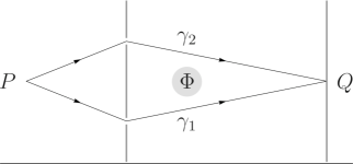
Figure 1: A plane projection of the standard magnetic Aharonov-Bohm effect apparatus.

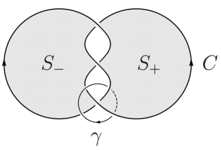
Figure 2: The trefoil knot $C$ bounds an oriented surface $S=S_{-}+S_{+}$ called the Seifert surface. The curve $\gamma$ passes through a hole in the Seifert surface.

In the standard Aharonov-Bohm effect, the two interfering paths of the electron and the solenoid are both copies of $S^{1}$ combined to form the Hopf link, topology of which is described by the fundamental group $\pi_{1}(S^{3}-S^{1})=\mathbb{Z}.$ The resulting Gaussian linking is distinguished by a single winding number. Generalization of the Aharonov-Bohm effect to a trefoil knotted solenoids [7], where the fundamental group $\pi_{1}(S^{3}-K)=\mathbb{Z}*\mathbb{Z}$ has a relation $\alpha^{3}=\beta^{2}$ between its generators, leads to the following results.

Consider a solenoid along path $C$ which bounds the surface $S=S_{-}+S_{+}$ called the Seifert surface as shown in Fig. 2, and a wave function along path $C^{\prime}$, not shown in Fig. 2. If the wave function along $C^{\prime}$ is a closed unknot that bounds the surface $D^{\prime}$ (also not shown) linked with a knotted solenoid $C$ (i.e., if $C^{\prime}$ punches through $S$), then

$$\phi=\oint_{C^{\prime}=\partial D^{\prime}}A\cdot dx=\int_{D^{\prime}}B\cdot dS=\frac{e\Phi}{\hbar c}.$$

On the other hand if the wave function is knotted and the solenoid is an unknot we find (interchanging paths $C$ and $C^{\prime}$)

$$\phi=\oint_{C=\partial S}A\cdot dx=\int_{S}B\cdot dS=\frac{e\Phi}{\hbar c}.$$

In both cases the Gaussian linking is determined by the number of times wave function path passes through oriented surface that bounds the solenoid. Note that if the wave function is linked through one of the holes in the Siefert surface, see path $\gamma$ in Fig. 2, then there is no Gaussian linking, and no standard Aharonov-Bohm effect, since there is no Gaussian linking. But the curves are nonetheless linked via higher order linking. It is rather difficult to explore higher order linking involving knots, so we will investigate a more tractable case. The simplest example of higher order linking is given by the Borromean rings. A generalization of the Aharonov-Bohm experiment of this type is shown in Fig. 3. After a careful choice of an appropriate gauge, one finds that the interference in the wave function along $C_{3}$ is proportional to the product of the fluxes in the two solenoids along $C_{1}$ and $C_{2}$,

$$\phi=\frac{e^{2}\Phi_{1}\Phi_{2}}{\hbar^{2}c^{2}}.$$

The analysis of The Josephson effect [9] has a related generalization [10], shown in Fig. 4, which results in the current maximum

$$I=I_{0}\lvert\cos{(2\pi^{2}\Phi_{1}\Phi_{2}/\Phi_{0}^{2})}\rvert$$

between points $P$ and $Q$ in the figure that is again proportional to the product of the fluxes in the two solenoids, where $\Phi_{0}$ is the fluxoid.

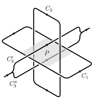
Figure 3: Schematic of a Borromean ring arrangement to detect the second order phase.

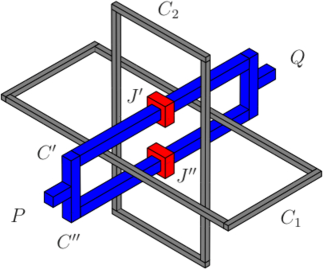
Figure 4: A schematic of a generalized magnetic Josephson effect apparatus. $J^{\prime}$ and $J^{\prime\prime}$ are Josephson junctions. $C_{1}$ and $C_{2}$ are solenoids.

5 Knots and links in quantum systems

There as many examples of quantum systems that support flux tubes, vortices, or other tube or line like structures. For instance, such systems include non-abelian gauge theories including quantum chromodynamics, superconductors, superfluids, liquid crystals, and atomic condensates to name a few.

Knots were first discussed in the context of particle physics by Lord Kelvin who modeled ÒelementraryÓ atoms as knotted fluid vortices in the aether. While this model did not succeed due to insufficient scientific knowledge at the time, it did show that Kelvin was ahead of his time.

6 Tightly knotted QCD flux tubes as glueballs

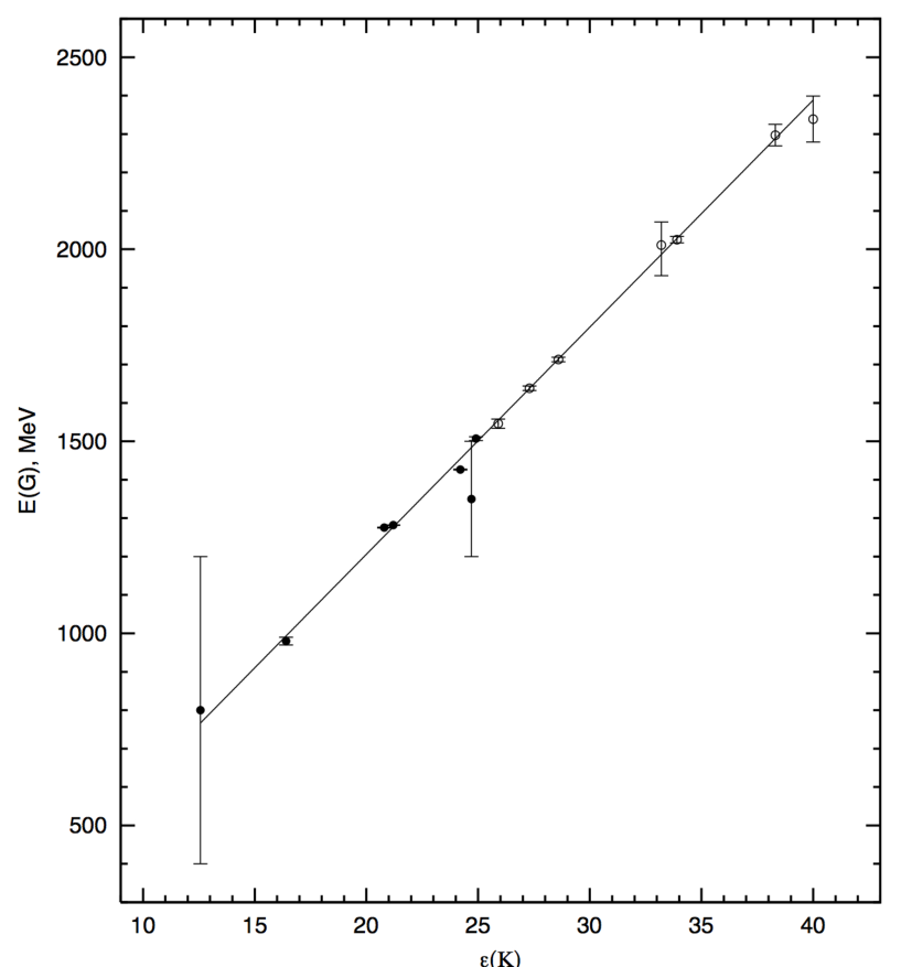
Figure 5: Relationship between the glueball spectrum E(G) and ratio of knot length to flux tube radius. Each point in this figure represents a glueball identified with a knot or link. The straight line is the model fit of $f_{J}$ states to the tight knot/link spectrum from [12], which contains more discussion.

The quark model is sufficient to describe most of the spectrum of hadronic bound states, but after filling the multiplets, a number of states remain and it has been suggested that at least one and perhaps several of these states are glueballs—states with no valance quarks. Two of us have suggested that the glueball spectrum of QCD is a result of tight knots and links of quantized chromo-electric flux [12]. This provides an infinite spectrum, up to stability, of new hadronic states, and predicts their energies. Identifying knot lengths with particle energies means the glueball spectrum is the same as the tight knot spectrum up to an overall scaling parameter. A fit matching knot/link lengths [13] with the presumed $f_{J}$ glueball states [14] states, is shown in Fig. 5, see Ref. [12], where the lightest $f_{J}$ state is identified with the shortest knot or link, the next lightest state with the next shortest knot or link, etc. E.g., we identify the $f_{0}(600)$ with the Hopf link, the $f_{0}(980)$ with the trefoil knot, etc. The fact that this is a one parameter fit means that any system of tightly knotted tubes will show the same universal behavior, with their energy/mass spectra corresponding to the length of knots and links up to one overall scaling parameter per system [12].

In the present model, glueball candidates of non-zero angular momentum, called $f_{J}$ states, correspond to spinning knots and links. (These solitonic objects could also have intrinsic angular momentum, but that will not be discussed here.) To calculate rotational energies we need the moment of inertia tensor for each tight knot and link. We can get exact results for links with planar components. E.g., in its center of mass frame, the moment of inertia tensor for a Hopf link of uniform density is

$${I_{\textrm{\scriptsize Hopf}}}=\left(\begin{array}[]{ccc}21&0&0\\ 0&\frac{75}{2}&0\\ 0&0&\frac{75}{2}\end{array}\right)\pi^{2}\rho\;a^{5},$$

where one torus is in the $xz$-plane and the other is in the $xz$-plane. Note this inertia tensor corresponds to a prolate spheroid as do other straight chains of links with an even number of elements. Odd straight chains do not have so much symmetry. Moment of inertia tensors of other knots and links can be calculated by Monte Carlo methods [13]. For further discussion and a detailed analysis of both the zero and non-zero angular momentum $f_{J}$ states including calculations of moment of inertia tensor see Ref. [15].

7 Conclusions

There are many classical systems that can be knotted or linked. Some of these knots can be tight, e.g., Taylor states in plasmas, but since the tubes can carry an arbitrary amount of flux, their radii are not fixed. In contrast, the flux in quantum systems is quantized leading to fixed radius tubes and hence quantized lengths for tight knots an links. This in turn leads to a quantized mass/energy spectrum. More generally, any quantum systems that supports quantized flux will have this same universal spectrum, i.e., one parameter per system—the slope.

References

References

- [1] V. Katritch, et al., Nature 384 (1996) 142; V. Katritch, et al., Nature 388 (1997) 148.
- [2] L. Woltjer, PNAS, 44, 489 (1958).
- [3] H. K. Moffatt, J. Fluid Mech. 35, 117 (1969).
- [4] J. B. Taylor, Phys. Rev. Lett, 33, 1139 (1974).
- [5] Y. Aharonov and D. Bohm, Phys. Rev. 115, 485 (1959).
- [6] A. Tonomura, N. Osakabe, T. Matsuda, T. Kawasaki, J. Endo, S. Yano, H. Yamada, Phys. Rev. Lett. 56, 792, (1986).
- [7] R. V. Buniy and T. W. Kephart, Phys. Lett. A 373, 919 (2009) [arXiv:0808.1891 [hep-th]].
- [8] The relevant topology can be found in D. Rolfsen, Knots and Links, Publish or Perish, Berkeley, California (1976).
- [9] B. D. Josephson, Physics Letters, 1, 251 (1962).
- [10] R. V. Buniy and T. W. Kephart, J. Phys. A (2010), to appear; arXiv:0808.1892 [hep-th].
- [11] R. V. Buniy and T. W. Kephart, Phys. Lett. A 372, 2583 (2008) [arXiv:hep-th/0611334] and R. V. Buniy and T. W. Kephart, Phys. Lett. A 372, 4775 (2008) [arXiv:hep-th/0611335].
- [12] R. V. Buniy and T. W. Kephart, Phys. Lett. B 576, 127 (2003) [arXiv:hep-ph/0209339]; R. V. Buniy and T. W. Kephart, Int. J. Mod. Phys. A 20, 1252 (2005) [arXiv:hep-ph/0408027]; R. V. Buniy and T. W. Kephart, Published in Physical and Numerical Models in Knot Theory Including Applications to the Life Sciences. Edited by J. Calvo, K.C. Millett, E.J. Rawdon and A. Stasiak. World Scientific, 2005. p. 45. arXiv:hep-ph/0408025.
- [13] T. Ashton, J. Cantarella, M. Piatek and E. Rawdon, arXiv:0508248 [math.DG].
- [14] C. Amsler et al. [Particle Data Group], Phys. Lett. B 667, 1 (2008).
- [15] Martha J. Holmes, Ph.D. dissertation, Vanderbilt University (2009).