Constraining Modified Gravity with Euclid

Abstract

Future proposed satellite missions as Euclid can offer the opportunity to test general relativity on cosmic scales through mapping of the galaxy weak lensing signal. In this paper we forecast the ability of these experiments to constrain modified gravity scenarios as those predicted by scalar-tensor and $f(R)$ theories. We found that Euclid will improve constraints expected from the PLANCK satellite on these modified gravity models by two orders of magnitude. We discuss parameter degeneracies and the possible biases introduced by modified gravity.

I Introduction

Understanding the nature of the current observed accelerated expansion of our universe is probably the major goal of modern cosmology. Two possible mechanisms can be at work: either our Universe is described by general relativity (GR, hereafter) and its energy content is dominated by a negative pressure component, coined ”dark energy”, either only ”standard” forms of matter exist and GR is not valid on cosmic scales (see e.g. Tsujikawa:2010sc , Silvestri:2009hh ).

All current cosmological data are consistent with the choice of a cosmological constant as dark energy component with equation of state $w=P/\rho=-1$ where $P$ and $\rho$ are the dark energy pressure and density respectively (see e.g. Serra:2009yp , Padmanabhan:2002ji , Peebles:2002gy ).

While deviations at the level of $\sim 10\%$ on $w$ assumed as constant are still compatible with observations and bounds on $w$ are even weaker if $w$ is assumed to be redshift-dependent, it may well be that future measurements will be unable to significantly rule out the cosmological constant value of $w=-1$.

Measuring $w$, however, is just part of the story. While the background expansion of the universe will be identical to the one expected in the case of a cosmological constant, the growth of structures with time could be significantly different if GR is violated. Modified gravity models have recently been proposed where the expansion of the universe is identical to the one produced by a cosmological constant, but where the primordial perturbations that will result in the large scale structures in the universe we observed today, grow at a different rate (see e.g. Laszlo:2007td , Amendola:2007rr , Linder:2007hg ).

Weak lensing measurements offer the great opportunity to map the growth of perturbations since they relate directly to the dark matter distribution and are not plagued by galaxy luminous bias (Bartelmann:1999yn , Refregier:2003ct , VanWaerbeke:2003uq ). Recent works have indeed make use of current weak lensing measurements, combined with other cosmological observables, to constrain modified gravity yielding no indications for deviations from GR (Daniel:2010ky , Lombriser:2010mp , Bean:2010zq , Zhao:2010dz , Daniel:2008et , Daniel:2009kr ).

Next proposed satellite mission as Euclid (Refregier:2010ss , Refregier:2006vt ) or WFIRST Gehrels:2010fn could measure the galaxy weak lensing signal to high precision, providing a detailed history of structure formation and the possibility to test GR on cosmic scales.

In this paper we study the ability of these future satellite missions to constrain modified gravity models and to possibly falsify a cosmological constant scenario. Respect to recent papers that have analyzed this possibility (e.g. Thomas:2008tp , Xia:2009gb ) we improve on several aspects. First of all, we forecast the future constraints by making use of Monte Carlo simulations on synthetic realisations of datasets. Previous analyses (see e.g. Amendola:2007rr , Zhao:2008bn , Heavens:2007ka ) often used the Fisher matrix formalism that, while fast, it may lose its reliability when Gaussianity is not respected due, for instance, to strong parameter degeneracies. Secondly we properly include the future constraints achievable by the Planck satellite experiment, also considering CMB lensing, that is a sensitive probe of modified gravity (see e.g. Serra:2009kp , Calabrese:2009tt and references therein). Thirdly, we discuss the parameter degeneracies and the impact of modified gravity on the determination of cosmological parameters,. Finally we focus on $f(R)$ and scalar-tensor theories, using the general parametrization proposed by Zhao:2008bn .

Our paper is structured as follows. In Section II we introduce the parametrization used to describe departures from GR, and then specialize to the case of $f(R)$ and scalar-tensor theories. In Section III we describe Galaxy weak-lensing, while in section IV we discuss how to extract lensing information from CMB data. We review the analysis method and the data forecasting in Section V. In Section VI we present our results and we derive our conclusions in Section VII.

II Modified gravity parametrization

In this section we describe the formalism we use to parametrize departures from general relativity.

II.1 Background expansion

In our analysis we fix the background expansion to a standard $\Lambda$CDM cosmological model. The reasons for this choice are multiple; $\Lambda$CDM is currently the best fit to available data and popular models of modified gravity, e.g. $f(R)$, closely mimic $\Lambda$CDM at the background level with differences which are typically smaller than the precision achievable with geometric tests Hu:2007nk . The most significant departures happen at the level of growth of structure and, by restricting ourselves to $\Lambda$CDM backgrounds, we are able isolate them.

II.2 Structure formation

In modified gravity models we expect departures from the standard growth of structure, even when the expansion history matches exactly the $\Lambda$CDM one. Dark matter clustering, as well as the evolution of the metric potentials, is changed and can be scale-dependent. Moreover, typically there might be an effective anisotropic stress introduced by the modifications and the two potentials appearing in the metric element, $\Phi$ and $\Psi$, are not necessarily equal, as is in the $\Lambda$CDM model. Here we focus on the effect of the modified evolution of the potential, $\Phi+\Psi$, on the CMB power spectra.
In order to study the potentials evolution and to evaluate the growth of perturbations in modified gravity models we employ the MGCAMB code developed in Zhao:2008bn (and publicly available at http://www.sfu.ca/~gza5/MGCAMB.html) . In this code the modifications to the Poisson and anisotropy equations are parametrized by two functions $\mu(a,k)$ and $\gamma(a,k)$ defined by:

$$k^{2}\Psi=-\frac{a^{2}}{2M_{P}^{2}}\mu(a,k)\rho\Delta\ ,\\$$ (1)

$$\frac{\Phi}{\Psi}=\gamma(a,k)\,,$$ (2)

where $\rho\Delta\equiv\rho\delta+3\frac{aH}{k}(\rho+P)v$ is the comoving density perturbation. These functions can be expressed using the parametrization introduced by Bertschinger:2008zb (and used in Zhao:2008bn ):

$$\mu(a,k)=\frac{1+\beta_{1}\lambda_{1}^{2}\,k^{2}a^{s}}{1+\lambda_{1}^{2}\,k^{2}a^{s}}\,,\\$$ (3)

$$\gamma(a,k)=\frac{1+\beta_{2}\lambda_{2}^{2}\,k^{2}a^{s}}{1+\lambda_{2}^{2}\,k^{2}a^{s}}\,,$$ (4)

where the parameters $\beta_{i}$ can be thought of as dimensionless couplings, $\lambda_{i}$ as dimensionful length scales and $s$ is determined by the time evolution of the characteristic length scale of the theory. $\Lambda$CDM cosmology is recovered for $\beta_{1,2}=1$ or $\lambda_{1,2}^{2}=0$ Mpc².

II.2.1 Scalar-Tensor theories

This parametrization can be to constrain chameleon type scalar-tensor theories, where the gravity Lagrangian is modified with the introduction of a scalar field Khoury:2003aq . As shown in Zhao:2008bn , for this kind of theories the parameters $\{\beta_{i},\lambda_{i}^{2}\}$ are related in the following way:

$$\beta_{1}=\frac{\lambda_{2}^{2}}{\lambda_{1}^{2}}=2-\beta_{2}\frac{\lambda_{2}^{2}}{\lambda_{1}^{2}}$$ (5)

and $1\lesssim s\lesssim 4$.
This implies that we can analyze scalar-tensor theories adding 3 independent parameters to the standard cosmological parameter set.

II.2.2 $f(R)$  theories

In the specific case of $f(R)$ theories we can additionally reduce the number of free parameters since $f(R)$ theories correspond to a fixed coupling $\beta_{1}=4/3$ Magnano:1993bd . Moreover, to have $\Lambda$CDM background expansion the $s$ parameter must be $\sim 4$ Zhao:2008bn . The parametrization in Eq. (3) effectively neglects a factor representing the rescaling of the Newton’s constant (e.g. $(1+f_{R})^{-1}$ in $f(R)$ theories) that, as pointed out in Giannantonio:2009gi , is very close to unity in models that satisfy local tests of gravity Hu:2007nk and so negligible. However, when studying the $f(R)$ case, we need to include it to get a more precise MCMC analysis (see Giannantonio:2009gi for the detailed expression of Eq. (3)). Even with this extended parametrization, we have only one free parameter left, the length scale $\lambda_{1}$. In this work we will constrain $f(R)$ theories through this parameter, evaluating the effects of these theories on gravitational lensing.

III Galaxy weak Lensing

Being sensitive the the growth rate of the structure, weak lensing can be very useful to constrain modified gravity and to distinguish between various modified gravity models when combined with CMB observations.
More generally, weak lensing (see Munshi:2006fn for a recent review or http://www.gravitationallensing.net) is a particularly powerful probe for Cosmology, since it simultaneously measures the growth of structure through the matter power spectrum, and the geometry of the Universe through the lensing effect. Since weak lensing probes the dark matter power spectrum directly, it is not limited by any assumption about the galaxy bias (how galaxies are clustered with respect to the dark matter) that represents one of the main limitations of galaxy surveys.
Following Bartelmann:1999yn one can describe the distortion of the images of distant galaxies through the tensor:

$\psi_{ij}=\left(\begin{array}[]{cc}-\kappa-\gamma_{1}&-\gamma_{2}\\ -\gamma_{2}&-\kappa+\gamma_{2}\\ \end{array}\right)$

where $\kappa$ and $(\gamma_{1},\gamma_{2})$ represents respectively the convergence (or magnification) and the shear (or stretching) component of the distortion. The reconstruction of matter density field can be conducted by looking at the correlations of the image distortions. The observable one has to deal with, will be hence a convergence power spectra kai:1992 ; Kaiser:1996tp :

$$P_{jk}(\ell)=H_{0}^{3}\int_{0}^{\infty}\frac{dz}{E(z)}W_{i}(z)W_{j}(z)P_{NL}[P_{L}\left(\frac{H_{0}\ell}{r(z)},z\right)]$$ (6)

where $P_{NL}$ is the non-linear matter power spectrum at redshift $z$, obtained correcting the linear one $P_{L}$. $W(z)$ is a weighting function, with subscripts $i$ and $j$ indicating the bins in redshifts. The function $W(z)$ also encodes the cosmological information, being:

$$W_{i}(z)=\frac{3}{2}\Omega_{m}(1+z)\int_{z_{i}}^{z_{i+1}}dz^{\prime}\frac{n_{i}(z^{\prime})r(z,z^{\prime})}{r(0,z^{\prime})}$$ (7)

where:

$$r(z,z^{\prime})=\int_{z}^{z^{\prime}}\frac{dz^{\prime}}{E(z^{\prime})}$$

with $E(z)=H(z)/H_{0}$ and $n_{i}(z^{\prime})$ is the fraction of sources belonging to the $i-th$ bin.
The observed convergence power spectra is affected mainly by a systematic arising from the intrinsic shear of galaxies $\gamma^{2}_{rms}$. This uncertainties can be reduced averaging over a large number of sources. The observed convergence power spectra will be hence:

$$C_{jk}=P_{jk}+\delta_{jk}\gamma^{2}_{rms}\tilde{n}_{j}^{-1}$$ (8)

where $\tilde{n}_{j}$ is the number of sources per steradian in the $j-th$ bin.

IV CMB lensing extraction

In the analysis we perform, we choose to introduce, in addition to galaxy weak lensing, the information derived from CMB lensing extraction.
Gravitational CMB lensing, as already shown in Ref. Perotto:2006rj , can improve significantly the CMB constraints on several cosmological parameters, since it is strongly connected with the growth of perturbations and gravitational potentials at redshifts $z<1$ and, therefore, it can break important degeneracies. The lensing deflection field $d$ can be related to the lensing potential $\phi$ as $d=\nabla\phi$ hirata:2003 . In harmonic space, the deflection and lensing potential multipoles follows:

$$d_{\ell}^{m}=-i\sqrt{\ell(\ell+1)}\phi_{\ell}^{m},$$ (9)

and therefore, the power spectra $C^{dd}_{\ell}\equiv\left\langle d_{\ell}^{m}d_{\ell}^{m*}\right\rangle$ and $C_{\ell}^{\phi\phi}\equiv\left\langle\phi_{\ell}^{m}\phi_{\ell}^{m*}\right\rangle$ are related through:

$$C_{\ell}^{dd}=\ell(\ell+1)C_{\ell}^{\phi\phi}.$$ (10)

Gravitational lensing introduces a correlation between different CMB multipoles (that otherwise would be fully uncorrelated) through the relation:

$$\left\langle a_{\ell}^{m}b_{\ell^{\prime}}^{m^{\prime}}\right\rangle=(-1)^{m}\delta_{m}^{m^{\prime}}\delta_{\ell}^{\ell^{\prime}}C_{\ell}^{ab}+\sum_{LM}{\Xi^{mm^{\prime}M}_{\ell\ \ell^{\prime}\ L}\phi^{M}_{L}}~{},$$ (11)

where $a$ and $b$ are the ${T,E,B}$ modes and $\Xi$ is a linear combination of the unlensed power spectra $\tilde{C}_{\ell}^{ab}$ (see lensextr for details).
In order to obtain the deflection power spectrum from the observed $C_{\ell}^{ab}$, we have to invert Eq. (11), defining a quadratic estimator for the deflection field given by:

$$d(a,b)_{L}^{M}=n_{L}^{ab}\sum_{\ell\ell^{\prime}mm^{\prime}}W(a,b)_{\ell\ \ell^{\prime}\ L}^{mm^{\prime}M}a^{m}_{\ell}b^{m^{\prime}}_{\ell^{\prime}}~{},$$ (12)

where $n_{L}^{ab}$ is a normalization factor needed to construct an unbiased estimator ($d(a,b)$ must satisfy Eq. (9)). This estimator has a variance:

$$\langle d(a,b)_{L}^{M*}d(a^{\prime},b^{\prime})_{L^{\prime}}^{M^{\prime}}\rangle\equiv\delta_{L}^{L^{\prime}}\delta^{M^{\prime}}_{M}(C_{L}^{dd}+N_{L}^{aa^{\prime}bb^{\prime}})$$ (13)

that depends on the choice of the weighting factor $W$ and leads to a noise $N_{L}^{aa^{\prime}bb^{\prime}}$ on the deflection power spectrum $C_{L}^{dd}$ obtained through this method. The choice of $W$ and the particular lensing estimator we employ will be described in the next section.

V Future data analysis

V.1 Galaxy weak lensing data

$n_{gal}(arcmin^{-2})$	$redshift$	$f_{sky}$	$\gamma^{2}_{rms}$
$35$	$0<z<2$	$0.5$	$0.22$

Table 1: Specifications for the Euclid like survey considered in this paper. The table shows the number of galaxies per square arcminute ($n_{gal}$), redshift range, $f_{sky}$ and intrinsic shear ($\gamma^{2}_{rms}$).

Future weak lensing surveys will measure photometric redshifts of billions of galaxies allowing the possibility of 3D weak lensing analysis (e.g.Heavens:2003 ; Castro:2005 ; Heavens:2006 ; Kitching:2007 ) or a tomographic reconstruction of growth of structures as a function of time through a binning of the redshift distribution of galaxies, with a considerable gain of cosmological information (e.g. on neutrinos Hannestad:2006as ; dark energy Kitching:2007 ; the growth of structure art:Bacon ; art:Massey and map the dark matter distribution as a function of redshift art:Taylor ).
Here we use typical specifications for futures weak lensing surveys like the Euclid experiment, observing about $35$ galaxies per square arcminute in the redshift range $0<z<2$ with an uncertainty of about $\sigma_{z}=0.03(1+z)$ (see Refregier:2006vt ), to build a mock dataset of convergence power spectra. Table 1 shows the number of galaxies per arcminute^-2 ($n_{gal}$), redshift range, $f_{sky}$ and intrinsic shear for this survey. The expected $1\sigma$ uncertainty on the convergence power spectra $P(\ell)$ is given by Cooray:1999rv :

$$\sigma_{\ell}=\sqrt{\frac{2}{(2\ell+1)f_{sky}\Delta_{\ell}}}\left(P(\ell)+\frac{\gamma_{rms}^{2}}{n_{gal}}\right)$$ (14)

For the convergence power spectra we use $\ell_{max}=1500$ in order to exclude the scales where the non-linear growth of structure is more relevant and the shape of the non-linear matter power spectra is, as a consequence, more uncertain (see Smith:2002dz ). We calculate the power spectra at a mean redshift $z=1$. $\Delta_{\ell}$ in the (14) is the bin used to generate data. Here we choose $\Delta_{\ell}=1$ for the range $2<\ell<100$ and $\Delta_{\ell}=40$ for $100<\ell<1500$.
In this first-order analysis we are not considering other systematic effects as intrinsic alignments of galaxies, selection effects and shear measurements errors due to uncertainties in the point spread function (PSF) determination. Of course future real data analysis will require the complete treatment of these effects in order to avoid biases on the cosmological parameters.

V.2 CMB data

We create a full mock CMB datasets (temperature, E–polarization mode and lensing deflection field) with noise properties consistent with the Planck :2006uk experiment (see Tab. 2 for specifications).

Experiment	Channel	FWHM	$\Delta T/T$
Planck	70	14’	4.7
	100	10’	2.5
	143	7.1’	2.2
$f_{sky}=0.85$

Table 2: Planck experimental specifications. Channel frequency is given in GHz, FWHM (Full-Width at Half-Maximum) in arc-minutes, and the temperature sensitivity per pixel in $\mu K/K$. The polarization sensitivity is $\Delta E/E=\Delta B/B=\sqrt{2}\Delta T/T$.

We consider for each channel a detector noise of $w^{-1}=(\theta\sigma)^{2}$, where $\theta$ is the FWHM (Full-Width at Half-Maximum) of the beam assuming a Gaussian profile and $\sigma$ is the temperature sensitivity $\Delta T$ (see Tab. 2 for the polarization sensitivity). We therefore add to each $C_{\ell}$ fiducial spectra a noise spectrum given by:

$$N_{\ell}=w^{-1}\exp(\ell(\ell+1)/\ell_{b}^{2})\,,$$ (15)

where $\ell_{b}$ is given by $\ell_{b}\equiv\sqrt{8\ln 2}/\theta$.

In this work, we use the method presented in lensextr to construct the weighting factor $W$ of Eq. (12). In that paper, the authors choose $W$ to be a function of the power spectra $C_{\ell}^{ab}$, which include both CMB lensing and primary anisotropy contributions. This choice leads to five quadratic estimators, with $ab={TT,TE,EE,EB,TB}$; the $BB$ case is excluded because the method of Ref. lensextr is only valid when the lensing contribution is negligible compared to the primary anisotropy, assumption that fails for the B modes in the case of Planck.
The five quadratic estimators can be combined into a minimum variance estimator which provides the noise on the deflection field power spectrum $C_{\ell}^{dd}$:

$$N_{\ell}^{dd}=\frac{1}{\sum_{aa^{\prime}bb^{\prime}}{(N_{\ell}^{aba^{\prime}b^{\prime}})^{-1}}}~{}.$$ (16)

We compute the minimum variance lensing noise for Planck experiment by means of a routine publicly available at http://lesgourg.web.cern.ch/lesgourg/codes.html. The datasets (which include the lensing deflection power spectrum) are analyzed with a full-sky exact likelihood routine available at the same URL.

V.3 Analysis method

In this paper we perform two different analysis. First, we evaluate the achievable constraints on the $f(R)$ parameter $\lambda_{1}^{2}$ and on the more general scalar-tensor parametrization including also $\beta_{1}$ and $s$. Secondly, we investigate the effects of a wrong assumption about the modified gravity on the cosmological parameters, by generating an $f(R)$ datasets with non-zero $\lambda_{1}^{2}$ fiducial value and analysing it fixing $\lambda_{1}^{2}=0$ Mpc². We conduct a full Monte Carlo Markov Chain analysis based on the publicly available package cosmomc Lewis:2002ah with a convergence diagnostic using the Gelman and Rubin statistics.
We sample the following set of cosmological parameters, adopting flat priors on them: the baryon and cold dark matter densities $\Omega_{b}h^{2}$ and $\Omega_{c}h^{2}$, the ratio of the sound horizon to the angular diameter distance at decoupling $\theta_{s}$, the scalar spectral index $n_{s}$, the overall normalization of the spectrum $A_{s}$ at $k=0.002$ Mpc^-1, the optical depth to reionization $\tau$, and, finally, the modified gravity parameters $\lambda_{1}^{2}$, $\beta_{1}$ and $s$.
The fiducial model for the standard cosmological parameters is the best-fit from the WMAP seven years analysis of Ref. wmap7 with $\Omega_{b}h^{2}=0.02258$, $\Omega_{c}h^{2}=0.1109$, $n_{s}=0.963$, $\tau=0.088$, $A_{s}=2.43\times 10^{-9}$, $\Theta=1.0388$.
For modified gravity parameters, we first assume a fiducial value $\lambda_{1}^{2}=0$ Mpc² and fix $\beta_{1}=1.33$ and $s=4$ to test the constraints achievable on the $f(R)$ model. We then repeat the analysis allowing $\beta_{1}$ and $s$ to vary. Furthermore, to investigate the ability of the combination of Planck and Euclid data to detect an hypothetical modified gravity scenario, we study a model with fiducial $\lambda_{1}^{2}=300$ Mpc² leaving $\lambda_{1}^{2}$, $\beta_{1}$ and $s$ as free variable parameters allowing them to vary in the ranges $0\leq\lambda_{1}^{2}\leq 10^{6}$, $0.1\leq\beta_{1}\leq 2$ and $1\leq s\leq 4$. Finally, we analyse a dataset with a fiducial value $\lambda_{1}^{2}=300$ Mpc² but assuming a wrong $\Lambda$CDM model fixing $\lambda_{1}^{2}=0$ Mpc², to investigate the bias introduced on the cosmological parameter due to a wrong assumption about the gravity model.

VI Results

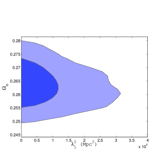
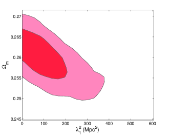
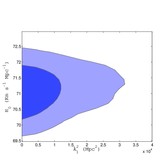
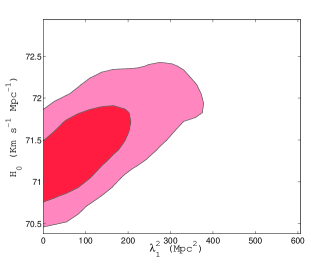
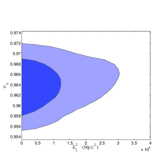
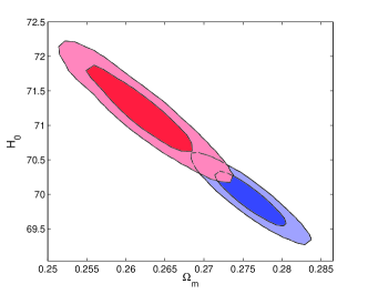
In Table 3 we show the MCMC constraints at $68\%$ c.l. for the $f(R)$ case for Planck alone and Planck combined with Euclid. For this last case we also fit the data fixing $\lambda_{1}^{2}$ to $0$, thus performing a standard analysis in a General Relativity framework, in order to show the importance of the degeneracies introduced by $\lambda_{1}^{2}$ on the other cosmological parameters errors. The parameters mostly correlated with modified gravity are $H_{0}$ and $\Omega_{c}h^{2}$ (see also Figure 1) because these parameters strongly affect the lensing convergence power spectrum as well as $\lambda_{1}^{2}$ through $P(k,z)$. As expected in fact, when assuming general relativity we find strong improvements on the errors on these parameters for the combination Planck+Euclid in comparison to the varying $\lambda_{1}^{2}$ analysis. We note that the constraints on the standard cosmological parameters are in good agreement with those showed in Refregier:2010ss .

	Planck	Planck+Euclid
Fiducial:	$\lambda_{1}^{2}=0$	$\lambda_{1}^{2}=0$	$\lambda_{1}^{2}=0$
Model:	varying $\lambda_{1}^{2}$	varying $\lambda_{1}^{2}$	fixed $\lambda_{1}^{2}$
Parameter
$\Delta{(\Omega_{b}h^{2})}$	$0.00013$	$0.00011$	$0.00010$
$\Delta{(\Omega_{c}h^{2})}$	$0.0010$	$0.00073$	$0.00057$
$\Delta{(\theta_{s})}$	$0.00027$	$0.00025$	$0.00023$
$\Delta{(\tau)}$	$0.0041$	$0.0030$	$0.0026$
$\Delta{(n_{s})}$	$0.0031$	$0.0029$	$0.0027$
$\Delta{(\log[10^{10}A_{s}])}$	$0.013$	$0.0091$	$0.0091$
$\Delta{(H_{0})}$	$0.50$	$0.38$	$0.29$
$\Delta{(\Omega_{\Lambda})}$	$0.0050$	$0.0040$	$0.0031$
$\lambda_{1}^{2}$(Mpc2)	$<2.42\times 10^{4}$	$<2.9\times 10^{2}$	$-$

Table 3: $68\%$ c.l. errors on cosmological parameters. Upper limits on $\lambda_{1}^{2}$ are $95\%$ c.l. constraints.
In the third column we show constraints on the cosmological parameters when fitting the data assuming general relativity, i.e. fixing $\lambda_{1}^{2}=0$ Mpc².

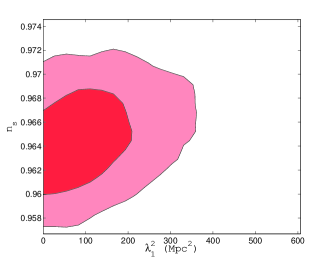
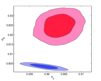
In Figure 1 we show the $68\%$ and $95\%$ confidence level 2-D likelihood contour plots in the $\Omega_{m}-\lambda_{1}^{2}$, $H_{0}-\lambda_{1}^{2}$ and $n_{s}-\lambda_{1}^{2}$ planes, for Planck on the left (blue) and Planck+Euclid on the right (red). As one can see the inclusion of Euclid data can improve constraints on the standard cosmological parameters from a $10\%$ to a $30\%$, with the most important improvements on the dark matter physical density and the Hubble parameter to which the weak lensing is of course very sensitive as showed by Eq. (6) and (7). Concerning modified gravity, Euclid data are decisive to constrain $\lambda_{1}^{2}$, improving of two order of magnitude the $95\%$ c.l. upper limit, thanks to the characteristic effect of the modified gravity on the growth of structures.

	Planck+Euclid	Planck+Euclid	Fiducial values
Model:	$\lambda_{1}^{2}=0$	varying $\lambda_{1}^{2}$
Parameter
$\Omega_{b}h^{2}$	$0.022326\pm 0.000096$	$0.02259\pm 0.00012$	$0.02258$
$\Omega_{c}h^{2}$	$0.1126\pm 0.00055$	$0.11030\pm 0.00083$	$0.1109$
$\theta_{s}$	$1.0392\pm 0.00023$	$1.0395\pm 0.00025$	$1.0396$
$\tau$	$0.0775\pm 0.0024$	$0.08731\pm 0.0029$	$0.088$
$n_{s}$	$0.9592\pm 0.0027$	$0.9636\pm 0.0029$	$0.963$
$H_{0}$	$69.94\pm 0.27$	$71.20\pm 0.42$	$71.0$
$\Omega_{\Lambda}$	$0.724\pm 0.003$	$0.738\pm 0.005$	$0.735$
$\sigma_{8}$	$0.8034\pm 0.0008$	$0.8245\pm 0.0039$	$0.8239$

Table 4: best fit value and $68\%$ c.l. errors on cosmological parameters for the case with a fiducial model $\lambda_{1}^{2}=300$ fitted with a $\Lambda$CDM model where $\lambda_{1}^{2}=0$ is assumed.

Moreover, when analyzing the $f(R)$ mock datasets with $\lambda_{1}^{2}=300$ Mpc² as fiducial model, assuming $\lambda_{1}^{2}=0$ Mpc² we found a consistent bias in the recovered best fit value of the cosmological parameters due to the degeneracies between $\lambda_{1}^{2}$ and the other parameters. As it can be seen from the comparison of Figures 1 and Figures 2 and from table 4 the shift in the best fit values is, as expected, along the degeneracy direction of the parameters with $\lambda_{1}^{2}$, for example for $n_{s}$, $H_{0}$ and $\Omega_{m}$. These results show that for an even small modified gravity, the best fit values recovered by wrongly assuming general relativity are more than $68\%$ c.l. (for some parameters at more than $95\%$ c.l.) away from the correct fiducial values, and may cause an underestimation of $n_{s}$ and $H_{0}$ and an overestimation of $\sigma_{8}$ and $\Omega_{m}$. More generally, as shown in table 4, all parameters are affected.
We conclude, hence, that a future analysis of so high precision data from Euclid and Planck will necessarily require to allow for possible deviations from general relativity, in order to not bias the best fit value of the cosmological parameters.

We also perform an analysis allowing $\beta_{1}$ and $s$ to vary; in this way we can constrain not only $f(R)$theories but also more general scalar-tensor models, adding to the standard parameter set the time variation of the new gravitational interaction $s$ and the coupling with matter $\beta_{1}$.
We perform this analysis assuming as a fiducial model a $f(R)$ theory with $\lambda_{1}^{2}=3.0\times 10^{4}$ Mpc² and $\beta_{1}=4/3$.

	Planck	Planck+Euclid
Fiducial:	$\lambda_{1}^{2}=3.0\times 10^{4}$	$\lambda_{1}^{2}=3.0\times 10^{4}$
Parameter
$\Delta{(\Omega_{b}h^{2})}$	$0.00013$	$0.00011$
$\Delta{(\Omega_{c}h^{2})}$	$0.0011$	$0.00082$
$\Delta{(\theta_{s})}$	$0.00026$	$0.00025$
$\Delta{(\tau)}$	$0.0043$	$0.0040$
$\Delta{(n_{s})}$	$0.0033$	$0.0029$
$\Delta{(\log[10^{10}A_{s}])}$	$0.014$	$0.011$
$\Delta{(H_{0})}$	$0.54$	$0.40$
$\Delta{(\Omega_{\Lambda})}$	$0.0060$	$0.0045$
$\Delta{(\beta_{1})}$	$0.13$	$0.038$
$\lambda_{1}^{2}$	unconstrained	unconstrained
$s$	unconstrained	unconstrained

Table 5: $68\%$ c.l. errors on cosmological parameters and $\beta_{1}$. We do not show limits on $\lambda_{1}^{2}$ and $s$ because this kind of analysis does not allow to constrain them (see text).

In Table 5 we report the $68\%$ c.l. errors on the standard cosmological parameters, plus the coupling parameter $\beta_{1}$. Performing a linear analysis, with a fiducial value of $\lambda_{1}^{2}=3\times 10^{4}$, we obtain constraints on $\beta_{1}$ with $\Delta{(\beta_{1})}=0.038$ at $68\%$ c.l. and therefore potentially discriminating between modified gravity models and excluding the $\beta_{1}=1$ case (corresponding to the standard $\Lambda$CDM model) at more than $5-\sigma$ from a combination of Planck+Euclid data (only $2-\sigma$ for Planck alone).
The strong correlation present between $\beta_{1}$ and $\lambda_{1}^{2}$ (see eq. 3) implies that, choosing a lower $\lambda_{1}^{2}$ fiducial value for a $f(R)$  model, the same variation of $\beta_{1}$ brings to smaller modifications of CMB power spectra and therefore we can expect weaker bounds on the coupling parameter. In order to verify this behaviour we made three analysis fixing $s=4$ and choosing three different fiducial values for $\lambda_{1}^{2}$: $3\times 10^{2}$, $3\times 10^{3}$ and $3\times 10^{4}$ Mpc². The respectively obtained $\beta_{1}$ $68\%$ c.l. errors are $0.11$, $0.052$ and $0.035$, confirming the decreasing expected accuracy on $\beta_{1}$ for smaller fiducial values of $\lambda_{1}^{2}$.

The future constraints presented in this paper are obtained using a MCMC approach. Since most of the forecasts present in literature on $f(R)$ theories are obtained using a Fisher matrix analysis, it is useful to compare our results with those predicted by a Fisher Matrix approach. We therefore perform a Fisher Matrix analysis for Planck and Planck+Euclid (see DeBernardis:2008ys ; Hannestad:2006as ; Bond:1997wr ) assuming a $\Lambda$CDM fiducial model and we compare the results with those in Table 3.
We find that for Planck alone the error on $\lambda_{1}$ is underestimated by a factor $\sim 3$ while the error is closer to the MCMC result for the Planck+Euclid case (underestimated by a factor $\sim 1.2$).

Figure 1: 2-dimensional contour plots showing the degeneracies at $68\%$ and $95\%$ confidence levels for Planck on the left (blue countours) and Planck+Euclid on the right (red countours).Notice different scale for abscissae.

Figure 2: 2-dimensional contour plots showing the degeneracies at $68\%$ and $95\%$ confidence levels for Planck+Euclid assuming a $f(R)$ fiducial cosmology with $\lambda_{1}^{2}=300$Mpc² considering an analysis with $\lambda_{1}^{2}$ fixed to $0$ (blue countours) or allowing it to vary (red countours).

VII Conclusions

In this paper we forecasted the ability of future weak lensing surveys as Euclid to constrain modified gravity. We restricted our analysis to models that could mimic a cosmological constant in the expansion of the Universe and can therefore be discriminated by only looking at the growth of perturbations. We have found that Euclid could improve the constraints on these models by nearly two order of magnitudes respect to the constraints achievable by the Planck CMB satellite alone. We have also discussed the degeneracies among the parameters and we found that neglecting the possibility of modified gravity can strongly affect the constraints from Euclid on parameters as the Hubble constant $H_{0}$, $\Omega_{m}$ and the amplitude of r.m.s. fluctuations $\sigma_{8}$. In this paper we found that, considering more general expansion histories, would further relax our constraints and increase the degeneracies between the parameters. However other observables can be considered as Baryonic Acoustic Oscillation and luminosity distances of high redshift supernovae to further probe the value of $w$ and its redshift dependence.

VIII Acknowledgments

It is a pleasure to thank Adam Amara and Luca Amendola for useful comments and suggestions. We also thank Gong-Bo Zhao for the latest version of the MGCAMB code. Support was given by the Italian Space Agency through the ASI contracts Euclid- IC (I/031/10/0)

References

- (1) S. Tsujikawa, arXiv:1004.1493 [astro-ph.CO].
- (2) A. Silvestri and M. Trodden, Rept. Prog. Phys. 72 (2009) 096901 [arXiv:0904.0024 [astro-ph.CO]].
- (3) P. Serra, A. Cooray, D. E. Holz, A. Melchiorri, S. Pandolfi and D. Sarkar, Phys. Rev. D 80 (2009) 121302 [arXiv:0908.3186 [astro-ph.CO]].
- (4) T. Padmanabhan, Phys. Rept. 380 (2003) 235 [arXiv:hep-th/0212290].
- (5) P. J. E. Peebles and B. Ratra, Rev. Mod. Phys. 75 (2003) 559 [arXiv:astro-ph/0207347].
- (6) I. Laszlo and R. Bean, Phys. Rev. D 77 (2008) 024048 [arXiv:0709.0307 [astro-ph]].
- (7) L. Amendola, M. Kunz and D. Sapone, JCAP 0804 (2008) 013 [arXiv:0704.2421 [astro-ph]].
- (8) E. V. Linder and R. N. Cahn, Astropart. Phys. 28 (2007) 481 [arXiv:astro-ph/0701317].
- (9) M. Bartelmann and P. Schneider, Phys. Rept. 340 (2001) 291 [arXiv:astro-ph/9912508].
- (10) A. Refregier, Ann. Rev. Astron. Astrophys. 41 (2003) 645 [arXiv:astro-ph/0307212].
- (11) L. Van Waerbeke and Y. Mellier, arXiv:astro-ph/0305089.
- (12) S. F. Daniel, E. V. Linder, T. L. Smith, R. R. Caldwell, A. Cooray, A. Leauthaud and L. Lombriser, Phys. Rev. D 81 (2010) 123508 [arXiv:1002.1962 [astro-ph.CO]].
- (13) L. Lombriser, A. Slosar, U. Seljak and W. Hu, arXiv:1003.3009 [astro-ph.CO].
- (14) R. Bean and M. Tangmatitham, Phys. Rev. D 81 (2010) 083534 [arXiv:1002.4197 [astro-ph.CO]].
- (15) G. B. Zhao et al., Phys. Rev. D 81 (2010) 103510 [arXiv:1003.0001 [astro-ph.CO]].
- (16) S. F. Daniel, R. R. Caldwell, A. Cooray and A. Melchiorri, Phys. Rev. D 77 (2008) 103513 [arXiv:0802.1068 [astro-ph]].
- (17) S. F. Daniel et al., Phys. Rev. D 80 (2009) 023532 [arXiv:0901.0919 [astro-ph.CO]].
- (18) A. Refregier, A. Amara, T. D. Kitching, A. Rassat, R. Scaramella, J. Weller and f. t. E. Consortium, arXiv:1001.0061 [astro-ph.IM].
- (19) A. Refregier et al., arXiv:astro-ph/0610062.
- (20) N. Gehrels, arXiv:1008.4936 [astro-ph.CO].
- (21) S. A. Thomas, F. B. Abdalla and J. Weller, Mon. Not. Roy. Astron. Soc. 395 (2009) 197 [arXiv:0810.4863 [astro-ph]].
- (22) J. Q. Xia, Phys. Rev. D 79 (2009) 103527 [arXiv:0907.4860 [astro-ph.CO]].
- (23) F. De Bernardis, L. Pagano, P. Serra, A. Melchiorri and A. Cooray, JCAP 0806 (2008) 013 [arXiv:0804.1925 [astro-ph]].
- (24) S. Hannestad, H. Tu and Y. Y. Y. Wong, JCAP 0606 (2006) 025 [arXiv:astro-ph/0603019].
- (25) J. R. Bond, G. Efstathiou and M. Tegmark, Mon. Not. Roy. Astron. Soc. 291 (1997) L33 [arXiv:astro-ph/9702100].
- (26) G. B. Zhao, L. Pogosian, A. Silvestri and J. Zylberberg, Phys. Rev. D 79 (2009) 083513 [arXiv:0809.3791 [astro-ph]].
- (27) A. F. Heavens, T. D. Kitching and L. Verde, Mon. Not. Roy. Astron. Soc. 380 (2007) 1029 [arXiv:astro-ph/0703191].
- (28) E. Calabrese, A. Cooray, M. Martinelli, A. Melchiorri, L. Pagano, A. Slosar and G. F. Smoot, Phys. Rev. D 80 (2009) 103516 [arXiv:0908.1585 [astro-ph.CO]].
- (29) P. Serra, A. Cooray, S. F. Daniel, R. Caldwell and A. Melchiorri, Phys. Rev. D 79 (2009) 101301 [arXiv:0901.0917 [astro-ph.CO]].
- (30) W. Hu and I. Sawicki, Phys. Rev. D 76 (2007) 064004 [arXiv:0705.1158 [astro-ph]].
- (31) E. Bertschinger and P. Zukin, Phys. Rev. D 78 (2008) 024015 [arXiv:0801.2431 [astro-ph]].
- (32) J. Khoury and A. Weltman, Phys. Rev. Lett. 93 (2004) 171104 [arXiv:astro-ph/0309300].
- (33) G. Magnano and L. M. Sokolowski, Phys. Rev. D 50 (1994) 5039 [arXiv:gr-qc/9312008].
- (34) T. Giannantonio, M. Martinelli, A. Silvestri and A. Melchiorri, JCAP 1004 (2010) 030 [arXiv:0909.2045 [astro-ph.CO]].
- (35) D. Munshi, P. Valageas, L. Van Waerbeke and A. Heavens, Phys. Rept. 462 (2008) 67 [arXiv:astro-ph/0612667].
- (36) N. Kaiser, Astrophys. J. 388 (1992) 272.
- (37) N. Kaiser, Astrophys. J. 498 (1998) 26 [arXiv:astro-ph/9610120].
- (38) L. Perotto, J. Lesgourgues, S. Hannestad, H. Tu and Y. Y. Y. Wong, JCAP 0610 (2006) 013 [arXiv:astro-ph/0606227].
- (39) C. M. Hirata and U. Seljak, Phys. Rev. D 68 (2003) 083002 [arXiv:astro-ph/0306354].
- (40) T. Okamoto and W. Hu, Phys. Rev. D 67 (2003) 083002 [arXiv:astro-ph/0301031].
- (41) A. F. Heavens, 2003, MNRAS, 323, 1327
- (42) P. G. Castro, A. F. Heavens, T. D. Kitching, 2005, Phys. Rev. D, 72, 3516
- (43) A. F. Heavens, T. D. Kitching, A. N. Taylor, 2006, MNRAS, 373, 105
- (44) T. D. Kitching, A. F. Heavens, A. N. Taylor, M. L. Brown, K. Meisenheimer, C. Wolf, M. E. Gray, D. J. Bacon, 2007, MNRAS, 376, 771
- (45) S. Hannestad, H. Tu and Y. Y. Y. Wong, JCAP 0606 (2006) 025 [arXiv:astro-ph/0603019].
- (46) Bacon, D.; et al.; 2003; MNRAS, 363, 723-733
- (47) Massey R.; et al.; 2007, ApJS, 172, 239
- (48) Taylor, A. N.; et al.; 2004, MNRAS, 353, 1176
- (49) A. R. Cooray, Astron. Astrophys. 348 (1999) 31 [arXiv:astro-ph/9904246].
- (50) [Planck Collaboration], arXiv:astro-ph/0604069.
- (51) E. Komatsu et al., arXiv:1001.4538 [astro-ph.CO].
- (52) R. E. Smith et al. [The Virgo Consortium Collaboration], Mon. Not. Roy. Astron. Soc. 341 (2003) 1311 [arXiv:astro-ph/0207664].
- (53) A. Lewis and S. Bridle, Phys. Rev. D 66, 103511 (2002) (Available from http://cosmologist.info.)
- (54) A. Refregier, A. Amara, T. D. Kitching, A. Rassat, R. Scaramella, J. Weller and f. t. E. Consortium, arXiv:1001.0061 [astro-ph.IM].
- (55) F. De Bernardis, L. Pagano, P. Serra, A. Melchiorri and A. Cooray, JCAP 0806 (2008) 013 [arXiv:0804.1925 [astro-ph]].
- (56) S. Hannestad, H. Tu and Y. Y. Y. Wong, JCAP 0606 (2006) 025 [arXiv:astro-ph/0603019].
- (57) J. R. Bond, G. Efstathiou and M. Tegmark, Mon. Not. Roy. Astron. Soc. 291 (1997) L33 [arXiv:astro-ph/9702100].