Hysteresis effects of changing parameters of noncooperative games

Abstract

We adapt the method used by Jaynes to derive the equilibria of statistical physics to instead derive equilibria of bounded rational game theory. We analyze the dependence of these equilibria on the parameters of the underlying game, focusing on hysteresis effects. In particular, we show that by gradually imposing individual-specific tax rates on the players of the game, and then gradually removing those taxes, the players move from a poor equilibrium to one that is better for all of them.

I Introduction

The Maximum Entropy (Maxent) principle is an information-theoretic formalization of Occam’s razor. It says that if we are given the expectation values of some functions of a system’s state, then we should predict that the associated distribution is the one with minimal information (i.e., maximal entropy) consistent with those expectations Cover and Thomas (1991); Mackay (2003). Maxent provides a succinct way to derive much of statistical physics Jaynes (1957); Jaynes and Bretthorst (2003), e.g., the canonical ensemble.

Noncooperative game theory Fudenberg and Tirole (1991); Myerson (1991); Osborne and Rubenstein (1994); Aumann and Hart (1992) is the foundation of conventional economics. It uses provided utility functions of a set of human “players” to predict how the players will model one another. It then uses this to predict the players’ joint behavior.

Many recent applications of statistical physics to economics analyze it at a coarse-grained level, bypassing its game-theoretic foundation. Here we build on Wolpert (2004) and apply Maxent to game theory, thereby introducing statistical physics techniques into the foundation of economics.

In this application of Maxent, there is a separate expectation value for each player. In contrast, when applying Maxent to derive the canonical ensemble, there is a single expectation value (of the system’s energy). Accordingly, rather than the canonical ensemble’s single Boltzmann distribution, involving a single Hamiltonian and a single “temperature”, we derive a separate Boltzmann distribution for each player, involving only that player’s utility function, and a “temperature” unique to that player. The players’ Boltzmann distributions are coupled, and the joint solution provides a bounded rationality version of the Nash equilibrium (NE) of game theory, where each player’s inverse temperature quantifies their rationality.

We analyze the dependence of this modified NE on the parameters of the underlying game, focusing on bifurcation behavior and hysteresis effects. In particular, we show how by gradually imposing taxes on the players, and then gradually removing them, the joint behavior of the players can be moved from a poor equilibrium to a Pareto-superior one. (This can even be done if we require that the players agree to each infinitesimal change in tax rates, since each such change increases every player’s expected utility.) This is particularly interesting given estimates that non-OECD countries could increase their wealth by one third by moving from their current equilibrium to a different one. Next we introduce three toy models of how a society can modify tax rates: via “socialism”, a “market”, or “anarchy”. We then compare these three models in terms of the associated discounted sum of total utilities along the path of tax rates.

II Background

Many different axiomatic arguments establish that the amount of syntactic information in a distribution $P(y)$ increases as the Shannon entropy of that distribution, $S(P)\equiv-\sum_{y}P(y)ln[P(y)]$ Jaynes (1957); Jaynes and Bretthorst (2003); Cover and Thomas (1991), decreases. This provides a way to formalize “Occam’s razor”: given limited prior data concerning $P(y)$, predict $P(y)$ is the distribution with minimal information (maximum entropy) consistent with that data. This formalization of Occam’s razor is called the maximum entropy principle (Maxent). When the data concerning $P(y)$ is expectation values of functions under $P$, Maxent has proven extremely accurate in domains ranging from signal processing to supervised learning Mackay (2003). Jaynes used it to derive statistical physics Jaynes (1957), e.g., having the data be the expected energy of a system or its expected number of particles of various types.

A finite, strategic form noncooperative game consists of a set of $N$ players, where each player $i$ has her own set of allowed pure strategies $X_{i}$ of size $|X_{i}|<\infty$. A mixed strategy is a distribution $q_{i}(x_{i})$ over $X_{i}$. The joint distribution over $X\equiv\varprod_{i}X_{i}$ is $q(x)=\prod_{i}q_{i}(x_{i})$, and is called a strategy profile.

Each player $i$ has a utility function $u_{i}:X\rightarrow{\mathbb{R}}$. So given strategy profile $q$, the expected utility of player $i$ is ${\mathbb{E}}(u_{i})=\sum_{x}\prod_{j}q_{j}(x_{j})u_{i}(x)$ where $q_{-i}(x_{-i})\equiv\prod_{j\neq i}q_{j}(x_{j})$. The Nash equilibrium (NE) is the strategy profile defined by having every player $i$ set $q_{i}$ to maximizes $i$’s expected utility, i.e., $\forall i,\ q_{i}={\mbox{argmax}}_{q^{\prime}_{i}}\bigg{[}\sum_{x}q^{\prime}_{i}(x_{i})q_{-i}(x_{-i})u_{i}(x)\bigg{]}$. In general, this set of coupled equations has multiple solutions.

A well-recognized problem of using the NE to predict real-world behavior is its assumption that every player chooses their optimal mixed strategy, which is called full rationality. This assumption is violated (often badly) in many experimental settings Camerer (2003); Starmer (2000). Our modified NE derived using Maxent accommodates such bounded rationality.

III Maxent and Quantal Response Equilibria

To predict what $q$ the players in a given $N$-player game $\Gamma$ will adopt, first pick one of the players, $i$. Consider a counter-factual situation, where $i$ has the same move space and utility function as in $\Gamma$, but rather than have a set of $N-1$ other humans set the distribution over $X_{-i}$, an inanimate stochastic system sets that distribution, to some $q_{-i}(x_{-i})$. In general, due to her limited knowledge of $q_{-i}$, limited computational power, etc., $i$ will choose a suboptimal $q_{i}$, i.e., $q_{i}\not\in{\mbox{argmax}}_{p_{i}}[{\mathbb{E}}_{p_{i}q_{-i}}(u_{i})]$. To quantify this bounded rationality, in analogy to Jaynes’ derivation of the canonical ensemble, constrain $q_{i}$ so that ${\mathbb{E}}_{q_{i},q_{-i}}(u_{i})$ has some (nonmaximal) value for the given $q_{-i}$. Then Maxent says

$$q_{i}(x_{i})\propto\exp{[\beta_{i}{\mathbb{E}}_{q_{-i}}(u_{i}\mid x_{i})]}.$$ (1)

where $\beta_{i}$ is the Lagrange parameter enforcing the constraint. Note that as $\beta_{i}\rightarrow\infty$, $i$ becomes increasingly rational, whereas as $\beta_{i}\rightarrow 0$, she becomes increasingly irrational.

Next, recall that by the axioms of utility theory von Neuman and Morgenstern (1944), all that player $i$ is concerned with in choosing her mixed strategy is the resultant expected utility. Accordingly, we presume that if the best $i$ can do is choose a particular $q_{i}$ when $q_{-i}$ is set by an inanimate system, she would also choose $q_{i}$ if she faces that same distribution $q_{-i}$ when it is set by other humans.

Generalizing, Maxent says that Eq. 1 should hold simulatenously for all $N$ players $i$, with player-specific Lagrange parameters. This gives a set of $N$ coupled non-linear equations for $q$. Brouwer’s fixed point theorem Aliprantis and Border (2006) guarantees that set always has a solution, and in general it has more than one.

This prediction for $q$ is not based on a model of bounded rational human behavior derived from experimental data. It is based on desiderata concerning the prediction process, not on a model of the system being predicted. Nonetheless, it is intriguing to note that maximizing Shannon entropy has a natural interpretation in terms of a common model of human bounded rationality, involving the cost of computation. To see this, recall that $-S(q_{i})$ measures the amount of information in the distribution $q_{i}$. Say we equate the cost to $i$ of computing $q_{i}$ with this amount of information. Then under Maxent, player $i$ minimizes the cost of computing her mixed strategy, subject to a constraint for the value of her expected utility that acts as an “aspiration level” . Under this interpretation, $\beta_{i}$ quantifies $i$’s cost of computing $q_{i}$, in units of expected utility. Future work involves incorporating experimental data concerning human behavior as additional constraints in the Maxent. (Other models of the cost of computation can be found in Fudenberg and Levine (1998); Hart (2005); Rubinstein (1998); Russell and Subramanian (1995); Georgeff et al. (1999).)

Solutions to our $N$ coupled equations for $q$ are typically called “logit Quantal Response Equilibria” (QRE) in game theory McKelvey and Palfrey (1995, 1996, 2008); Anderson et al. (2002). They have been independently suggested several times as a way to model human players Shamma and Arslan (2004); Fudenberg and Kreps (1993); Fudenberg and Levine (1998); Meginniss (1976); Anderson et al. (2004); Durlauf (1999). In all this earlier work the logit distribution is not derived from first principles. Nor is it related to information theory, or the cost of computation. Rather typically the logit QRE has been used as an ad hoc, few-degree of freedom model of bounded rational play. As such it has been widely and successfully used to fit experimental data concerning human behavior.

IV The shape of the QRE surface

To analyze the QRE surface of Eq. 1, we express it as a set of functional relationships, $q_{i}=f_{i}(q_{-i},\beta_{i}),\quad q_{-i}=f_{-i}(q_{i},\beta_{-i})$. A bifurcation may occur if for some $i$

$$\frac{\partial f_{i}}{\partial q_{-i}}\frac{\partial f_{-i}}{\partial q_{i}}\frac{\partial q_{i}}{\partial\beta_{i}}+\frac{\partial f_{i}}{\partial\beta_{i}}-\frac{\partial q_{i}}{\partial\beta_{i}}=0$$ (2)

cannot be solved for $\frac{\partial q_{i}}{\partial\beta_{i}}$, i.e., if $\det(\frac{\partial f_{i}}{\partial q_{-i}}\frac{\partial f_{-i}}{\partial q_{i}}-\text{Id})=0$. To illustrate this and related phenomena, we consider games between a Row and Column player, each with two pure strategies. The first is the famous “battle of the sexes” coordination game Fudenberg and Tirole (1991), where the utility functions are

$$2|1 \;\;\;0|0$$

$$0|0 \;\;\;1|2$$ (3)

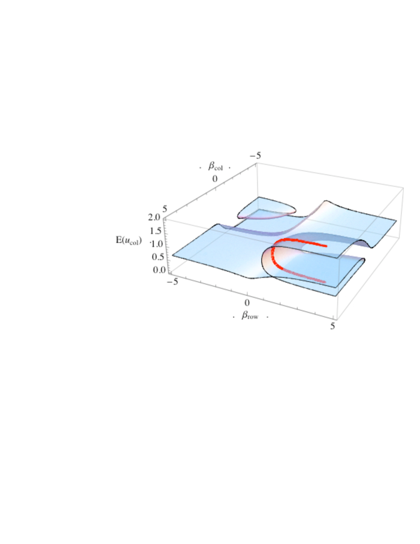
where the first (second) entry in each cell is the Row (Column) player’s utility for the associated pure strategy profile. Each joint inverse temperature ${\vec{\beta}}\equiv(\beta_{row},\beta_{column})$ fixes QRE $q$’s for this game, and therefore QRE expected utilities. Fig. 1 plots this surface taking $\vec{\beta}$ to ${\mathbb{E}}_{q}(u_{col})$. At bifurcations the number of QRE solutions changes between one and three, and infinitesimal changes in $\vec{\beta}$ may result in discontinuous changes in expected utility. (E.g., this happens if the system starts at $\vec{\beta}=(5,5)$ on the top surface, and then $\beta_{row}$ is reduced to $0$.)

Figure 1: ${\mathbb{E}}(u_{col})$ vs. $\vec{\beta}$ under the QRE of the game in Eq. 3. The hysteresis path involving bonds discussed in the text is highlighted.

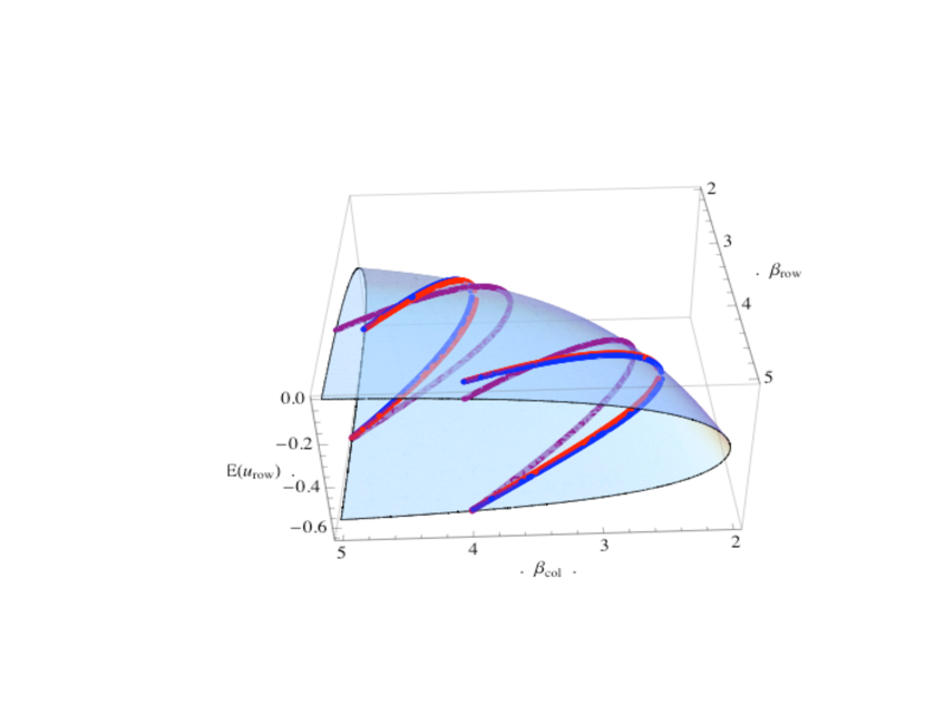
An interesting effect occurs if we multiply the utilities by $-1$. Fig. 3 illustrates part of the surface after this switch. Note that on the bottom fold, for fixed $\beta_{col}$, decreasing $\beta_{row}$ increases ${\mathbb{E}}(u_{row})$. So Row benefits by being less rational, due to how Column responds to Row’s drop in rationality.

Figure 2: The expected utility of the Row player along the path through $\vec{\beta}$ highlighted in Fig. 1, illustrated as a function of the Row player’s rationality, $\beta_{row}$. The path starts at the bottom right, then travels left, before turning and finishing at the top right. Even though the Row player ultimately benefits if society follows this path, at the beginning they lose expected utility. They may demand to be compensated for that initial drop, e.g., with proceeds of a bond that are paid off by both players when the end of the path is reached.

By Eq. 1, changing $\beta_{i}$ affects the QRE $q$ the same way as keeping $\beta_{i}$ fixed but multiplying $u_{i}$ by some $\alpha_{i}$. So Fig.’s 1, 3 give QRE surfaces where $\vec{\beta}$ is fixed, but each $u_{i}$ is multiplied by $\alpha_{i}$. (Formally, reinterpret the $x$ and $y$ axes as $\alpha_{row}$ and $\alpha_{col}$ rescaled, and reinterpret the $z$ axis as ${\mathbb{E}}_{q}(u_{i})/\alpha_{i}$.) Note we can interpret $1-\alpha_{i}$ as a tax rate on player $i$. So if we model rationalities $\beta_{i}$ as fixed, e.g., as behavioral attributes, then on the bottom surface in Fig. 3, Row benefits if her tax rate increases.

The fact that Row may prefer a higher tax rate suggests that by varying tax rates “adiabatically” slowly, so that the joint behavior of the players is always on the QRE surface, we may be able to montonically improve expected utilities for both players. Indeed, by changing tax rates we can gradually move the equilibrium across the surface from one fold to the other, and then undo those changes, returning the rates to their original values, but leaving both players with higher expected utility. (See  Wolpert and Kulkarni (2008) for other work that exploits the shape of a QRE surface to optimize player joint behavior.)

More precisely, there are paths of $\vec{\beta}$’s (i.e, of $\vec{\alpha}$’s) such that:

1. Neither player ever is more rational (taxed at a higher rate) on the path than at the starting point.

2. At each step on the path, if after the next infinitesimal change in $\vec{\beta}$ there is a QRE $q$ infinitesimally close to the current one, it is adopted. (Adiabaticity.)

3. Each infinitesimal change in $\vec{\beta}$ increases both ${\mathbb{E}}_{q}(u_{i})$’s.

4. At each infinitesimal step, if multiple changes in $q$ meet (1)-(3), but one is Pareto superior to the others (i.e., better for both players), the players coordinate on that one.

Examples of such paths are illustrated in Fig. 3.

The existence of such paths raises the question of how a society should dynamically update its tax rates. We now compare three procedures for how this could be done by society as a whole. (For notational simplicity, and to emphasize the analogy with annealing, we parameterize the procedures in terms of their action on $\vec{\beta}$ rather than on $\vec{1}-\vec{\alpha}$.)

1. “Anarchy”: Players independently decide how to modify their $\beta$’s. To do this they follow gradient ascent with a small step size $\Delta$, subject to the constraint that no player $i$ can go to a $\beta_{i}$ larger than the starting one. Thus, both players $i$ change $\beta_{i}$ by $\delta\beta_{i}\in[-\Delta,\Delta]$, using $\partial{\mathbb{E}}(u_{i})/\partial\beta_{i}$ to make their choice of what value $\delta\beta_{i}$ to pick. (Since this is a linear procedure, the players will always choose one of the three values $\{-\Delta,0,\Delta\}$.)

2. “Socialism”: An external regulator determines the path, again using gradient descent, this time over the sum of the players’ expected utilities. At each step of the path $\vec{\beta}$ is changed by the $(\delta\beta_{row},\delta\beta_{col})$ vector that maximizes

   $$[\delta\beta_{row}\frac{\partial{\mathbb{E}}(u_{row})}{\partial\beta_{row}}+\delta\beta_{col}\frac{\partial{\mathbb{E}}(u_{row})}{\partial\beta_{col}}]+[\delta\beta_{row}\frac{\partial{\mathbb{E}}(u_{col})}{\partial\beta_{row}}+\delta\beta_{col}\frac{\partial{\mathbb{E}}(u_{col})}{\partial\beta_{col}}]$$

   subject to $||(\delta\beta_{row},\delta\beta_{col})||^{2}\leq 2\Delta^{2}$. (The constraint is to match the step size to that of the first procedure.)

3. “Market”: Certain mild axioms concerning bargaining behavior of humans give a unique prediction for what bargain is reached in any bargaining scenario. Let $T$ be the set of joint expected utilities for all the bargains that a set of $N$ bargainers might reach in a particular bargaining scenario. Then the “Nash bargaining concept” Myerson (1991); Osborne and Rubenstein (1994) predicts that the the joint expected utility of the bargain reached is ${\mbox{argmax}}_{{\vec{u}}\in T}[\prod_{i=1}^{N}u_{i}]$.

   We can use the Nash bargaining concept to predict what change to $\vec{\beta}$ the players would agree to under a “market” where they bargain with one another to determine that change. To do this we fix the set of all allowed bargains to the set of all pairs ${\vec{\beta}}$ such that $||{\vec{\beta}}-{\vec{\beta}}(t)||^{2}\leq 2\Delta^{2}$, where ${\vec{\beta}}(t)$ is the current joint $\beta$. We also choose $\vec{d}$ to be the joint expected utility at ${\vec{\beta}}(t)$. So under Nash bargaining, at each iteration $t$, the players choose the change in joint $\beta$, $\delta{\vec{\beta}}$, that maximizes the product

   $$\bigg{[}{\mathbb{E}}(u_{Row}\mid{\vec{\beta}}(t)+\delta{\vec{\beta)}}-{\mathbb{E}}(u_{Row}\mid{\vec{\beta}}(t))\bigg{]}\;\times$$

   $$\bigg{[}{\mathbb{E}}(u_{Col}\mid{\vec{\beta}}(t)+\delta{\vec{\beta}})-{\mathbb{E}}(u_{Col}\mid{\vec{\beta}}(t))\bigg{]}$$

   subject to $||\delta{\vec{\beta}}||\leq 2\Delta^{2}$. As in the other two procedures, we use first order approximations in this one, to evaluate the two differences in expected utilities.

In all three procedures the total change in $\vec{\beta}$ in any step never exceeds $\sqrt{2}\Delta$. This adiabaticity reduces the computational burden on the players, by not changing the game too much from one timestep to the next. (Similar assumptions are called comparitive statics in economics Kehoe (1987).)

As in standard economics, we can quantify how good a full path produced by a procedure is for society as a whole by calculating the discounted sum of future utilities along the path,

$$Q \equiv \sum_{t^{\prime}>0}(1+\gamma)^{t-t^{\prime}}\sum_{i=1}^{N}{\mathbb{E}}(u_{i}(t^{\prime}))$$ (4)

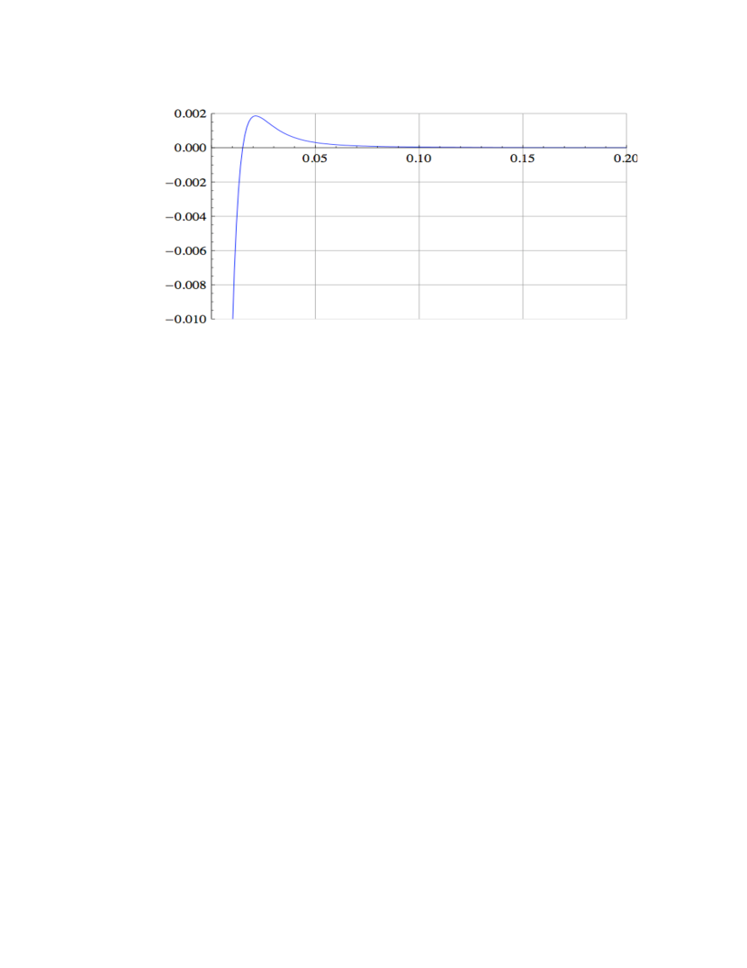
So we can compare the three procedures by calculating the $Q$’s for the paths they generate starting from some shared $\vec{\beta}$ at time $t=0$. We did this for several representative initial $\vec{\beta}$’s for the surface in Fig. 3. Anarchy always did worse than the other two procedures. Those others are compared to each other in Fig. 4. When the discounting factor $\gamma$ is large (i.e., we are more concerned with near-term than long-term utility) the market procedure does better, otherwise socialism does.

Figure 3: A QRE surface with paths shown for the anarchy (red), socialism (blue) and market (purple) procedures. As in Fig. 1, the x and y axes are player rationalities, $\beta_{row}$ and $\beta_{col}$, and the z axis is expected utility (this time of player Row).

Figure 4: The difference between the discounted sums of future expected utilities of the two players under the “socialism” and “market” procedures, plotted against the discounting factor $\gamma$.

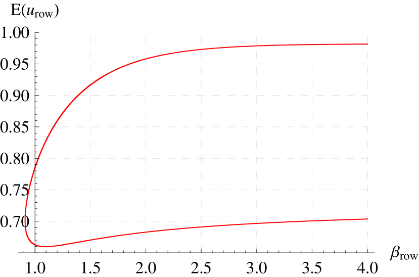
All three procedures are local, looking only a single step into the future. A procedure that also considers the QRE surface’s global geometry will produce better paths in general. In particular, such global information allows us to consider paths where a player loses expected utility for certain periods, but in the end all players are better off. Fig. 1 highlights such a path, along which player Column always benefits but player Row loses initially, before ultimately benefitting. (A cross-section of the expected utility of Row along the path is shown in Fig. 2. ) Note that player Row might demand compensation to agree to follow such a path where they temporarily lose expected utility,, e.g. in terms of a subsidy paid for with a bond that is repaid by all players at the end of the path.

Particularly interesting issues arise when setting full paths under the market model, if the players use discounted sum of future utilities to value full paths. For example, say that at $t=0$ society starts to follow a path $\vec{\beta}_{0}(t)$ that is a Nash bargaining solution then. Then in general, for $t^{\prime}>0$, the path $\vec{\beta}_{t^{\prime}}(t)$ that is a Nash bargaining solution for full paths starting from $\vec{\beta}_{0}(t^{\prime})$ is not a truncation of $\vec{\beta_{0}}(t)$ to $t>t^{\prime}$. There is an inconsistency across time. This raises many interesting issues concerning binding commitments, what it means for a path chosen by bargaining to be renegotiation-proof, etc.

Multiple folds will exist for the QRE surfaces involving many kinds of game parameters, not just tax rates. Often such parameters will be set externally, perhaps in a noisy process. When this is the case, the QRE surface tells us how stable player behavior is against that external noise. For example, say the players are on the top fold of the surface in Fig. 1, with $\vec{\beta}=(2,4)$, so the joint behavior is near an edge of the QRE surface. In this situation, small external noise may lead the players to “fall off the edge”, and undergo a discontinuous jump to the lower surface. Moreover, even if the players managed to (adiababitically slowly) restore their original rationalities after such a jump, they would end up on the middle fold of the region where $\beta_{row}$ is near $2$, not on the good fold they started in. Due to this, when an economic situation exhibits such qualitative features, it may behoove society to stay away from such edges in the QRE surface, even if that lowers total expected utility.

References

- Cover and Thomas (1991) T. Cover and J. Thomas, Elements of Information Theory (Wiley-Interscience, New York, 1991).
- Mackay (2003) D. Mackay, Information Theory, Inference, and Learning Algorithms (Cambridge University Press, 2003).
- Jaynes (1957) E. T. Jaynes, Physical Review 106, 620 (1957).
- Jaynes and Bretthorst (2003) E. T. Jaynes and G. L. Bretthorst, Probability Theory : The Logic of Science (Cambridge University Press, 2003).
- Fudenberg and Tirole (1991) D. Fudenberg and J. Tirole, Game Theory (MIT Press, Cambridge, MA, 1991).
- Myerson (1991) R. B. Myerson, Game theory: Analysis of Conflict (Harvard University Press, 1991).
- Osborne and Rubenstein (1994) M. Osborne and A. Rubenstein, A Course in Game Theory (MIT Press, Cambridge, MA, 1994).
- Aumann and Hart (1992) R. Aumann and S. Hart, Handbook of Game Theory with Economic Applications (North-Holland Press, 1992).
- Wolpert (2004) D. H. Wolpert, in Complex Engineered Systems: Science meets technology, edited by D. Braha, A. Minai, and Y. Bar-Yam (Springer, 2004) pp. 262–290.
- Camerer (2003) C. Camerer, Behavioral Game Theory: Experiments in Strategic Interaction (Princeton University Press, 2003).
- Starmer (2000) C. Starmer, Journal of Economic Literature 38, 332 (2000).
- von Neuman and Morgenstern (1944) J. von Neuman and O. Morgenstern, Theory of Games and Economics Behavior (Princeton university Press, 1944).
- Aliprantis and Border (2006) C. Aliprantis and K. C. Border, Infinite Dimensional Analysis (Springer Verlag, 2006).
- Fudenberg and Levine (1998) D. Fudenberg and D. K. Levine, The Theory of Learning in Games (MIT Press, Cambridge, MA, 1998).
- Hart (2005) S. Hart, Econometrica 73, 1401 (2005).
- Rubinstein (1998) A. Rubinstein, Modeling Bounded Rationality (MIT press, 1998).
- Russell and Subramanian (1995) S. Russell and D. Subramanian, Journal of AI Research , 575 (1995).
- Georgeff et al. (1999) M. Georgeff, B. Pell, M. Pollack, M. Tambe, and M. Wooldridge, in Intelligent Agents V, Lecture Notes in Computer Science, Vol. 1555 (Springer, Berlin / Heidelberg, 1999) pp. 1–10.
- McKelvey and Palfrey (1995) R. D. McKelvey and T. R. Palfrey, Games and Economic Behavior 10, 6 (1995).
- McKelvey and Palfrey (1996) R. D. McKelvey and T. R. Palfrey, Japanese Economic Review 47, 186 (1996).
- McKelvey and Palfrey (2008) R. D. McKelvey and T. R. Palfrey, in Handbook of Experimental Economics Results, Vol. 1 (North Holland, 2008) pp. 541–548.
- Anderson et al. (2002) S. P. Anderson, J. Goeree, and C. A. Holt, Southern Economic Journal 69, 21 (2002).
- Shamma and Arslan (2004) J. Shamma and G. Arslan, IEEE Trans. on Automatic Control 50, 312 (2004).
- Fudenberg and Kreps (1993) D. Fudenberg and D. Kreps, Games and Economic Behavior 5, 320 (1993).
- Meginniss (1976) J. R. Meginniss, Proceedings of the American Statistical Association, Business and Economics Statistics Section , 471 (1976).
- Anderson et al. (2004) S. P. Anderson, J. Goeree, and C. A. Holt, Scandanavian journal of economics , 21 (2004), preprint title was “Stochastic game th eory: adjustment to equilibrum under noisy directional learning.
- Durlauf (1999) S. Durlauf, Proceedings Natl. Acad. Sci. USA 96, 10582 (1999).
- Train (2003) K. E. Train, Discrete Choice Methods with Simulation (Cambridge University Press, 2003).
- Crites and Barto (1996) R. H. Crites and A. G. Barto, in Advances in Neural Information Processing Systems - 8, edited by D. S. Touretzky, M. C. Mozer, and M. E. Hasselmo (MIT Press, 1996) pp. 1017–1023.
- Hu and Wellman (1998) J. Hu and M. P. Wellman, in Proceedings of the Fifteenth International Conference on Machine Learning (1998) pp. 242–250.
- Wolpert and Tumer (2002) D. H. Wolpert and K. Tumer, Journal of Artificial Intelligence Research 16, 359 (2002).
- Wolpert et al. (2004) D. H. Wolpert, K. Tumer, and E. Bandari, Physical Review E 69 (2004).
- Wolpert and Kulkarni (2008) D. Wolpert and N. Kulkarni, in Proceedings of the 2008 NASA/ESA Conference on Adaptive Hardware and Systems, edited by A. Erdogan (IEEE Press, 2008).
- Kehoe (1987) T. J. Kehoe, in The New Palgrave: A Dictionary of Economics, edited by J. Eatwell, M. Milgate, and P. Newman (Palgrave Macmillan, 1987) pp. 517–520.