Traffic Network Optimum Principle – Minimum Probability of Congestion Occurrence

Abstract

We introduce an optimum principle for a vehicular traffic network with road bottlenecks. This network breakdown minimization (BM) principle states that the network optimum is reached, when link flow rates are assigned in the network in such a way that the probability for spontaneous occurrence of traffic breakdown at one of the network bottlenecks during a given observation time reaches the minimum possible value. Based on numerical simulations with a stochastic three-phase traffic flow model, we show that in comparison to the well-known Wardrop’s principles the application of the BM principle permits considerably greater network inflow rates at which no traffic breakdown occurs and, therefore, free flow remains in the whole network.

I Introduction

Under small enough network inflow rates, drivers move at their desired (or permitted) speeds. Usually, there are several alternative routes from an origin to a destination in a network for which travel times are different but close to each other. When network inflow rates increase considerably, traffic congestion occurs due to traffic breakdown causing a sharply increase in the route travel times. Thus one of the theoretical problems of traffic networks is to find an optimal feedback dynamic traffic network assignment between alternative routes that prevents traffic breakdown under great enough network inflow rates while maintaining free flow in the network (see, e.g., review Rakha2008 ). Traffic breakdown occurs mostly at a bottleneck and leads to the emergence of spatiotemporal congested traffic patterns. The bottleneck can result from on- and off-ramps, a road gradient, etc.

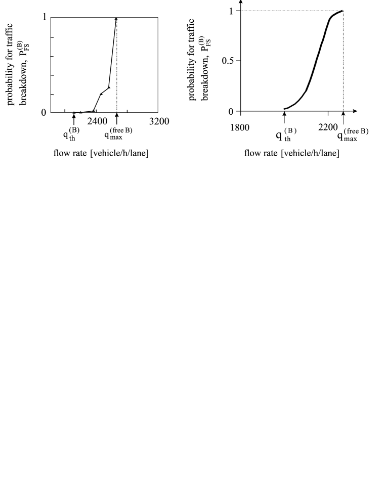
An empirical feature of traffic breakdown at a bottleneck is as follows KernerBook ; KernerBook2 . Traffic breakdown is a local first-order phase transition from free flow to synchronized flow (F$\rightarrow$S transition). The feature has been explained in three-phase traffic theory KernerBook in which there are three phases: 1. Free flow (F). 2. Synchronized flow (S). 3. Wide moving jam (J). Synchronized flow and wide moving jam are associated with congested traffic. A wide moving jam exhibits the characteristic jam feature to propagate through bottlenecks while maintaining the mean velocity of the downstream jam front. In contrast, the downstream front of synchronized flow is often fixed at the bottleneck. It has been found that there is a broad range $q^{\rm(B)}_{\rm th}\leq q\leq q^{\rm(free\ B)}_{\rm max}$ FlowMaxMin of the link (arc) flow rate $q$ within which free flow at the bottleneck is in a metastable state with respect to traffic breakdown (Fig. 1). The greater the flow rate $q$ in comparison with $q^{\rm(B)}_{\rm th}$, the smaller the critical amplitude of a disturbance in free flow whose growth leads to the breakdown, i.e., the greater the probability $P^{\rm(B)}_{\rm FS}$ of the breakdown occurrence during a given observation time $T_{\rm ob}$. At $q<q^{\rm(B)}_{\rm th}$ probability $P^{\rm(B)}_{\rm FS}=$ 0, i.e., no traffic breakdown occurs, while at the maximum flow rate $q=q^{\rm(free\ B)}_{\rm max}$ traffic breakdown occurs already due to a small disturbance, i.e., with probability $P^{\rm(B)}_{\rm FS}=$ 1.

Figure 1: Empirical (a) and simulated (b) probability of traffic breakdown at an on-ramp bottleneck. Fig. (a) is taken from Persaud et al. Persaud . Fig. (b) is taken from Fig. 4.2 of KernerBook2 . In (a) the averaging time interval for traffic variables $T_{\rm av}=$ 10 min TOB . In (b) the observation time of traffic flow $T_{\rm ob}=$ 15 min.

Most network optimization theories (see e.g., Rakha2008 ; Dif ; Wahle ; Davis ; Davis1 ) are based on the application of user equilibrium (UE) and system optimum (SO) principles introduced by Wardrop Wardrop : (i) Wardrop’s UE principle: traffic on a network distributes itself in such a way that the travel times on all routes used from any origin to any destination are equal, while all unused routes have equal or greater travel times. (ii) Wardrop’s SO principle: the network-wide travel time should be a minimum. The Wardrop’s principles reflect either the wish of drivers to reach their destinations as soon as possible (UE) or the wish of network operators to reach the minimum network-wide travel time (SO).

However, the Wardrop’s principles do not take into account that with some probability traffic breakdown occurs in the network, when the link flow rate for one of the network bottlenecks exceeds $q^{\rm(B)}_{\rm th}$. This breakdown leads usually to spatiotemporal congestion propagation KernerBook ; KernerBook2 . Such congestion growth within the network causes the associated growth of link travel times; as a result, under congestion conditions as has been shown by Wahle and Schreckenberg with colleagues Wahle and Davis Davis ; Davis1 ; Davis2 usually no true Wardrop’s equilibrium can be found.

In this article, we introduce a network breakdown minimization (BM) principle based on the empirical features of traffic breakdown. The application of the BM principle should minimize probability of congestion occurrence in the whole network. We show that the BM principle leads to considerably greater network inflow rates at which free flows remain in the network than under application of the Wardrop’s SO and UE principles.

II Network breakdown minimization (BM) principle

The BM principle is as follows:

• The optimum of a traffic network with $M$ links and $N$ bottlenecks is reached, when link inflow rates are assigned in the network in such a way that the probability

  $$P^{\rm(N)}_{\rm FS,net}=1-\prod^{\rm N}_{k=1}(1-P^{\rm(B,{\it k})}_{\rm FS})$$ (1)

  for spontaneous occurrence of traffic breakdown at one of the network bottlenecks during a given observation time $T_{\rm ob}$ reaches the minimum possible value, i.e., the network optimum is reached at

  $$\min_{q_{1},q_{2},...,q_{\rm M}}\{P^{\rm(N)}_{\rm FS,net}(q_{1},q_{2},...,q_{\rm M})\}.$$ (2)

  In (1), (2), $q_{m}$ is the link inflow rate for a link with index $m$; $m=1,2,...,M$, where $M>1$; $k=1,2,...,N$ is bottleneck index , $N>1$; $P^{\rm(B,{\it k})}_{\rm FS}$ is probability that during the time interval $T_{\rm ob}$ traffic breakdown occurs at bottleneck $k$. The BM principle (2) can be applied as long as free flow conditions remain in the network. In general, the BM principle (2) is devoted to the optimization of large, complex vehicular traffic networks consisting of a great number of links $M\gg 1$.

The BM principle (2) is equivalent to

$$\max_{q_{1},q_{2},...,q_{\rm M}}\{P^{\rm(N)}_{\rm C,net}(q_{1},q_{2},...,q_{\rm M})\},$$ (3)

where

$$P^{\rm(N)}_{\rm C,net}=\prod^{\rm N}_{k=1}P^{\rm(B,{\it k})}_{\rm C}$$ (4)

is the probability that during time interval $T_{\rm ob}$ free flows remain in the network, i.e., that traffic breakdown occurs at none of the bottlenecks; $P^{\rm(B,{\it k})}_{\rm C}=1-P^{\rm(B,{\it k})}_{\rm FS}$.

For a complete formulation of the optimization principle (2) (or (3)), link flow rates $q_{\rm m}$ should be connected with network inflow rates. To reach this goal in a general case of a dynamic traffic assignment in a traffic network, one should use a dynamic traffic flow model Rakha2008 . This dynamic model should calculate spatiotemporal dynamics of vehicular traffic variables within the network under given network inflow rates that can be time-functions.

However, for the simplicity of simulations of the BM principle (2) discussed below in Sec. III, we will use here a static traffic assignment for which the following well-known constraints are applied Rakha2008 :

$$\sum_{i}{\varphi^{rw}_{i}}=q_{rw}\quad\forall\ r,w,$$ (5)

$$\varphi^{rw}_{i}\geq 0\quad\forall\ i,r,w,$$ (6)

$$q_{m}=\sum_{r}{\sum_{w}{\sum_{i}{\varphi^{rw}_{i}\delta^{rw}_{m,i}}}}\quad\forall\ m,$$ (7)

where $q_{rw}$ is the total flow rate of vehicles going from origin $r$ to destination $w$; $\varphi^{rw}_{i}$ is the flow rate of vehicles going from $r$ to $w$ on route (path) $i$;

$$\delta^{rs}_{m,i}=\left\{\begin{array}[]{ll}1&\textrm{if link $m$ is on route $i$}\\ 0&\textrm{otherwise}.\end{array}\right.$$ (10)

III Simulations: Comparison of the BM and Wardrop’s principles

III.1 Model

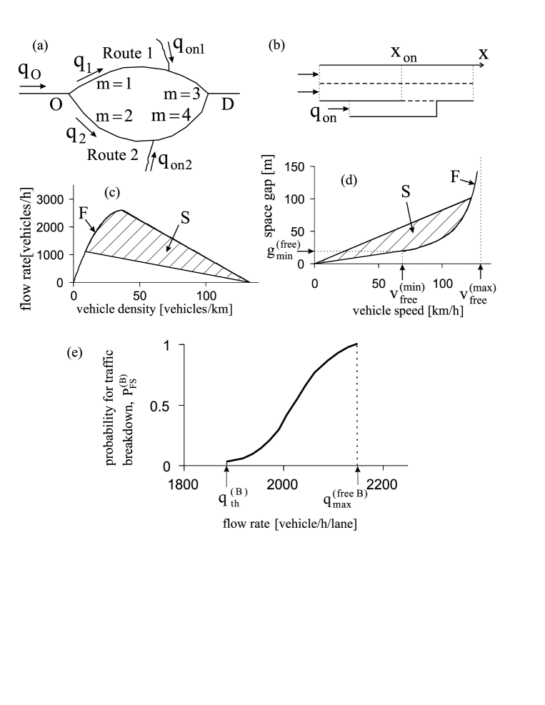
We compare the BM (2) and Wardrop’s principles through their application for a simple network with only two alternative routes 1 and 2 with lengths $L_{1}$ and $L_{2}$ (with $L_{2}>L_{1}$) for vehicles moving from origin $O$ to destination $D$ (Fig. 2 (a)) used often for studies of traffic control with Wardrop’s principles Wahle ; Davis ; Davis1 ; Davis2 .

Figure 2: Explanation of model: (a, b) Sketch of a simple network with two routes 1, 2 (a) and a route model (b); bottleneck parameters are the same as those in KKl2003A ; KKl2009 ; KKl2010 . (c, d) Model steady states in the flow–density (c) and space-gap–speed planes (d); F – free flow, S – synchronized flow. (e) Probability of spontaneous traffic breakdown at on-ramp bottleneck as function of the flow rate downstream of the bottleneck at $q_{\rm on}=$ 1000 vehicles/h for $T_{\rm ob}=$ 40 min.

In our model, we assume that routes 1 and 2 are two-lane roads with on-ramp bottlenecks (Fig. 2 (b)) whose on-ramp inflow rates $q_{\rm on1}$ and $q_{\rm on2}$ are given constants. Thus the network optimization is performed only through the assignment of a network inflow with the rate $q_{\rm O}$ between links $m=1,2$ on routes $i=1,2$ (Fig. 2 (a)). We designate link flow rates and travel times, respectively, as follows: for links $m=1,3$ on route 1 by $q_{\rm 1}$, $q_{\rm 3}$ and $T_{1,1}$, $T_{3,1}$; for links $m=2,4$ on route 2 by $q_{2}$, $q_{4}$ and $T_{2,2}$, $T_{4,2}$ (Fig. 2 (a)), where $q_{3}=q_{1}+q_{\rm on1}$, $q_{4}=q_{2}+q_{\rm on2}$. Travel times on routes 1 and 2 are $T_{1}=T_{1,1}+T_{3,1}$ and $T_{2}=T_{2,2}+T_{4,2}$, respectively. The BM principle (2) as well as Wardrop’s UE and SO principles can be written respectively as follows:

$${\rm BM:}\quad\min_{q_{1},q_{2}}\{1-(1-P^{\rm(B,1)}_{\rm FS}(q_{1}+q_{\rm on1}))(1-$$ (11)

$$-P^{\rm(B,2)}_{\rm FS}(q_{2}+q_{\rm on2}))\},\ q_{1}+q_{2}=q_{\rm O},$$

$${\rm UE:}\quad T_{1}(q_{1},q_{\rm on1})=T_{2}(q_{2},q_{\rm on2}),\ q_{1}+q_{2}=q_{\rm O},$$ (12)

$${\rm SO:}\quad\min_{q_{1},q_{2}}\{q_{1}T_{1,1}+(q_{1}+q_{\rm on1})T_{3,1}+q_{2}T_{2,2}+$$ (13)

$$+(q_{2}+q_{\rm on2})T_{4,2}\},\ q_{1}+q_{2}=q_{\rm O}.$$

Travel times $T_{1,1}$, $T_{3,1}$, $T_{2,2}$, $T_{4,2}$ are found via probe vehicles leaving the related links. These travel times are used in the UE (12) and SO (13) principles for calculations of $q_{1}$, $q_{2}$ as long as the probe vehicles have moved in free flows; this explains why only the associated time intervals are shown in related figures below Timelag .

For simulations, we use a discrete version KKl2009 of the Kerner-Klenov stochastic three-phase traffic flow model of KKl2003A that shows the empirical features of traffic breakdown including the resulting flow-dependence of breakdown probability $P^{\rm(B)}_{\rm FS}$ (Fig. 2 (e)) used in (11) GM_model . The model reads as follows:

$$v_{n+1}=\max(0,\min(v_{{\rm free},n},\tilde{v}_{n+1}+\xi_{n},v_{n}+a\tau,v_{{\rm s},n})),$$ (14)

$$x_{n+1}=x_{n}+v_{n+1}\tau,$$ (15)

where $n=0,1,2,...$ is number of time steps, $\tau$ is a time step, $x_{n}$ and $v_{n}$ are the vehicle coordinate and speed at time step $n$, $a$ is the maximum acceleration, $\tilde{v}_{n}$ is the vehicle speed without speed fluctuations $\xi_{n}$, $v_{{\rm s},n}$ is a safe speed.

The physics of this model as well as initial and boundary conditions used in simulations have already been considered in detail in Sec. 16.3 of the book KernerBook . In accordance with the fundamental hypothesis of three-phase traffic theory KernerBook ; KernerBook2 , steady states of synchronized flow cover a 2D-region in the flow–density plane (Fig. 2 (c)). Speed fluctuations $\xi_{n}$, functions $\tilde{v}_{n}$, $v_{{\rm s},n}$, rules for lane changing and model parameters used here are taken from KKl2010 (see Appendix A). The one exception from the model version of KKl2010 is that a free flow speed $v_{{\rm free},n}$ rather than to be a constant depends on space gap $g_{n}$ to the preceding vehicle:

$$v_{{\rm free},n}=v_{\rm free}(g_{n}),$$ (16)

where

$$v_{\rm free}(g)=\max[v_{\rm free}^{\rm(max)}(1-\kappa d/(g+d)),v_{\rm free}^{\rm(min)}],$$ (17)

$\kappa$, $v_{\rm free}^{\rm(max)}$ are given constants, $v_{\rm free}^{\rm(min)}$ (Fig. 2 (d)) is constant found from the equations

$$v^{\rm(free)}_{\rm min}=g^{\rm(free)}_{\rm min}/\tau,$$ (18)

$$v^{\rm(free)}_{\rm min}=v_{\rm free}(g^{\rm(free)}_{\rm min}).$$ (19)

III.2 Critical flow rate for traffic breakdown

In simulations, we study the spontaneous occurrence of traffic breakdown at one of the bottlenecks in the network (Fig. 2 (a)) during a given observation time $T_{\rm ob}=$ 40 min (where $T_{\rm ob}>T_{1},\ T_{2}$) at given on-ramp inflow rates $q_{\rm on1}$, $q_{\rm on2}$ under network optimization based on the application of each of the principles (11), (12), and (13).

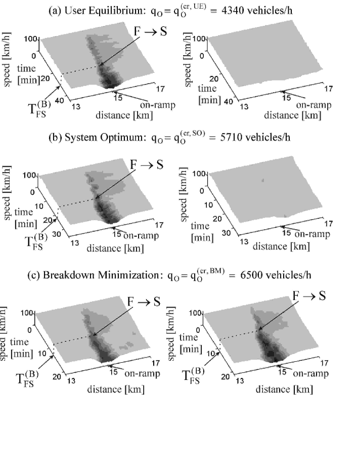
Figure 3: Traffic breakdown under application of UE (12) (a), SO (13) (b) and BM principles (11) (c), respectively. Speed in time and space in the right lane on route 1 (left) and route 2 (right). In (a) $q_{1}=3250$, $q_{2}=1090$, $q^{\rm(cr,\ UE)}_{\rm O}=$ 4340 vehicles/h. In (b) $q_{1}=$ 3250, $q_{2}=$ 2460, $q^{\rm(cr,\ SO)}_{\rm O}=$ 5710 vehicles/h. In (c) $q^{\rm(cr,\ BM)}_{\rm O}=$ 6500 vehicles/h. $T^{\rm(B)}_{\rm FS}$ is a random time delay of traffic breakdown labeled by arrows F$\rightarrow$S: $T^{\rm(B)}_{\rm FS}=$ 30 (a), 21 (b), 13 (route 1) and 11 (route 2) (c) min. $q_{\rm on1}=q_{\rm on2}=$ 1000 vehicles/h; road location of on-ramp bottleneck $x_{\rm on}=$ 15 km; $L_{1}=$ 20, $L_{2}=$ 25 km.

We find that a critical flow rate $q_{\rm O}=q^{\rm(cr)}_{\rm O}$ for traffic breakdown at one of the network bottlenecks, i.e., the inflow rate $q_{\rm O}$ at which the breakdown occurs with probability $P^{\rm(B)}_{\rm FS}=1$ on route 1 or/and 2 in the network (Fig. 2 (a)) Realization , satisfies conditions

$$q^{\rm(cr,\ BM)}_{\rm O}>q^{\rm(cr,\ SO)}_{\rm O}>q^{\rm(cr,\ UE)}_{\rm O},$$ (20)

where superscripts BM, UE, and SO are related to (11), (12), and (13), respectively.

Under application of Wardrop’s UE principle (12), most vehicles move on the route 1 because it is shorter, i.e., $q_{1}>q_{2}$. This explains why traffic breakdown occurs on route 1 (Fig. 3(a)). At the same flow rate $q_{\rm O}=$ 4340 vehicles/h, under application of the BM principle (11) we find $P^{\rm(B,{\it k})}_{\rm FS}=0$ for $k=$ 1 and 2, because for the BM principle (11) values $q_{1}+q_{\rm on1}$ and $q_{2}+q_{\rm on2}=$ 3170 vehicles/h are smaller than $q^{\rm(B)}_{\rm th}\approx$ 3760 vehicles/h (i.e., $q^{\rm(B)}_{\rm th}\approx$ 1880 vehicles/h/lane, Fig. 2 (e)).

As the UE principle (12), the SO principle (13) leads also to $q_{1}>q_{2}$; however, the difference $q_{1}-q_{2}$ is not great; therefore, the critical flow rate increases (Fig. 3 (b)). At the same flow rate $q_{\rm O}=$ 5710 vehicles/h, under application of the BM principle (11) we find $P^{\rm(B,{\it k})}_{\rm FS}=$ 0.05 for $k=1,2$; however, even when traffic breakdown occurs, the resulting congested patterns exists only during about 10 min dissolving later due to a return S$\rightarrow$F transition (simulations made are not shown here).

The greatest critical flow rate $q^{\rm(cr,\ BM)}_{\rm O}=$ 6500 vehicles/h is found for the BM principle (11); in this case, traffic breakdown occurs on both routes 1 and 2 (Fig. 3 (c)) ApBM .

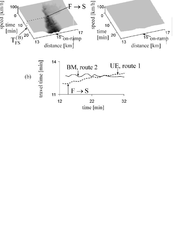
Figure 4: Comparison of travel times under application of Wardrop’s UE (12) and BM (11) principles at $q_{\rm O}=$ 4680 vehicles/h: (a) Speed in the right lane in space and time for route 1 (left) and 2 (right) under application of (12) ($q_{1}=$ 3360, $q_{2}=$ 1320 vehicles/h). (b) Time-dependences of travel times on route 1 for (12) (dashed curve) and on route 2 for (11) (solid curve). $T^{\rm(B)}_{\rm FS}=$ 15 min. Under application of (11), $P^{\rm(B,{\it k})}_{\rm FS}=0,\ k=1,2$. Other parameters are the same as those in Fig. 3.

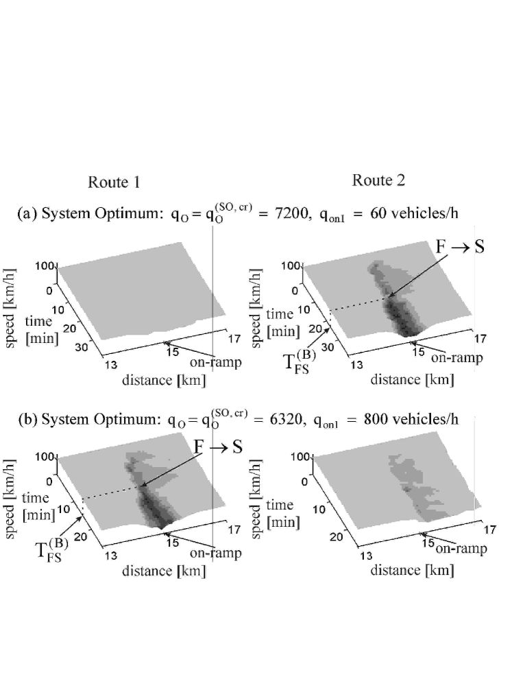
Figure 5: Change in route on which breakdown occurs with probability $P^{\rm(B)}_{\rm FS}=1$ under asymmetric bottleneck parameters and application of SO principle (13): (a) Traffic breakdown on route 2. (b) Traffic breakdown on route 1. $q_{\rm on2}=$ 1050 vehicles/h. $(q_{\rm on1},\ q^{\rm(cr,\ SO)}_{\rm O})=$ (60, 7200) (a), (800, 6320) (b) vehicles/h. $q^{\rm(ch)}_{\rm on1}\approx$ 350 vehicles/h. $L_{2}=$ 23 km. $T^{\rm(B)}_{\rm FS}=$ 22 (a) and 15 (b) min. Under application of (11), $P^{\rm(B,{\it k})}_{\rm FS}<1$ for $k=1,2$. Other parameters are the same as those in Fig. 3.

Thus in comparison with Wardrop’s UE and SO principles, the advantage of the BM principle (11) is the smaller traffic breakdown probability at the same network inflow rate and, therefore, the greater critical network inflow rate. The disadvantage of the BM principle (11) is that more drivers move on route 2 with a longer travel time. However, this disadvantage is true at small enough network inflow rates only. At greater network inflow rates, because of traffic congestion resulting from traffic breakdown under application of the Wardrop’s UE and SO principles, we find a quick growth of travel time on the shorter route 1. The greater network inflow rate exceeds the critical rate, the shorter the mean time delay of traffic breakdown and the quicker the growth of congestion.

For an example shown in Fig. 4, under application of Wardrop’s UE principle (12) due to congestion on route 1 travel time on this route becomes as long as under application of the BM principle (11) Timelag .

Above we have used symmetric bottleneck parameters $q_{\rm on1}=q_{\rm on2}$ for which under application of Wardrop’s principles traffic breakdown occurs always on the shorter route 1 (Figs. 3 and 4). Under asymmetric bottleneck parameters, we find the effect of change in route on which traffic breakdown can occur (Fig. 5): When $q_{\rm on1}\ll q_{\rm on2}$, traffic breakdown occurs on the longer route 2 (Fig. 5(a)), whereas at considerably greater flow rates $q_{\rm on1}$ traffic breakdown occurs on route 1 (Fig. 5(b)) as that in Figs. 3 and 4. Thus for a given $q_{\rm on2}$, there is a single flow rate $q_{\rm on1}=q^{\rm(ch)}_{\rm on1}(q_{\rm on2})$ for which $P^{\rm(B,1)}_{\rm FS}=P^{\rm(B,2)}_{\rm FS}$, i.e., $q^{\rm(cr,\ SO)}_{\rm O}=q^{\rm(cr,\ BM)}_{\rm O}=$ 6900 vehicles/h; however, for all other flow rates $q_{\rm on1}$ condition (20) is valid.

IV BM principle and traffic optimization at single bottleneck

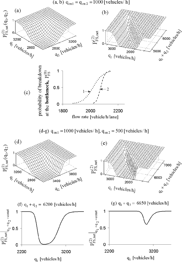
Breakdown probability at any single bottleneck exhibits no minimum: the breakdown probability is always a monotonously increasing flow rate function (Fig. 2 (e)). For this reason, the minimization of breakdown probability $P^{\rm(B)}_{\rm FS}$ for a single bottleneck is not possible. However, the minimization of breakdown probability $P^{\rm(N)}_{\rm FS,net}$ (1) for a traffic network is possible, as formulated in the BM principle of Sect. II.

Figure 6: Comparison of BM principle and traffic optimization at single bottleneck: (a, b) Probability of traffic breakdown $P^{\rm(2)}_{\rm FS,net}$ in the network with two bottlenecks shown in Fig. 2 (a) (i.e., when in Eq. (1) the value $N=2$) as a function of the flow rates $q_{1}$ and $q_{2}$ (a) and a function of the flow rates $q_{1}$ and $q_{\rm O}=q_{1}+q_{2}$ (b) for symmetric bottleneck parameters $q_{\rm on1}=q_{\rm on2}=$ 1000 [vehicles/h]. (c) Probability of traffic breakdown $P^{\rm(B)}_{\rm FS}$ at a single on-ramp bottleneck as a function of the flow rate downstream of the bottleneck for on-ramp inflow rates $q_{\rm on}=$ 1000 [vehicles/h] (curve 1 that is the same as that in Fig. 2 (e)) and $q_{\rm on}=$ 500 [vehicles/h] (curve 2). (d, e) $P^{\rm(2)}_{\rm FS,net}$ as functions of $q_{1}$ and $q_{2}$ (d) and of $q_{1}$ and $q_{\rm O}=q_{1}+q_{2}$ (e) for asymmetric bottleneck parameters $q_{\rm on1}=$ 1000 and $q_{\rm on2}=$ 500 [vehicles/h]. (f, g) $P^{\rm(2)}_{\rm FS,net}$ as a function of $q_{1}$ for different given values $q_{\rm O}=q_{1}+q_{2}=$ 6200 (f) and 6650 (g) [vehicles/h] associated with figure (e).

To understand the sense of this conclusion, we consider the simple network shown in Fig. 2 (a). There are two different bottlenecks in this case and, therefore, traffic assignment in the network changes breakdown probabilities for both bottlenecks. For this reason, although breakdown probability for each of the bottlenecks separately has no minimum, there is a minimum in breakdown probability $P^{\rm(N)}_{\rm FS,net}$ (1) for the network (Fig. 6 (a, b)).

Thus the BM principle for the optimization of a traffic network is conceptionally different in comparison with known traffic optimization approaches at a single bottleneck, in particular, with on-ramp metering.

Figures 6 (a, b) correspond to symmetric bottleneck parameters in the network shown in Fig. 2 (a); this explains why the minimum of breakdown probability in the network is related to the condition $q_{1}=q_{2}$ (Fig. 6 (a)). However, breakdown probability at the on-ramp bottleneck $P^{\rm(B)}_{\rm FS}$ depends on the on-ramp inflow rate considerably (Fig. 6 (c)). For this reason, under asymmetric bottleneck parameters the minimum of breakdown probability $P^{\rm(N)}_{\rm FS,net}$ in the network shown in Fig. 2 (a) is usually related to condition $q_{1}\neq q_{2}$ (Fig. 6 (d, f, g)).

V Conclusions

1. The network breakdown minimization (BM) principle introduced in the article states that the network optimum is reached, when link flow rates are assigned in the network in such a way that the probability for spontaneous occurrence of traffic breakdown at one of the network bottlenecks during a given observation time reaches the minimum possible value; this is equivalent to the maximization of probability that traffic breakdown occurs at none of the network bottlenecks. We have shown that the maximum network inflow rate at which free flows still remain in the network is considerably greater under application of the BM principle than that under application of the Wardrop’s UE or SO principles.

2. A traffic network optimization that is consistent with the empirical features of traffic breakdown of Sect. I can consist of the stages:

(i) The minimization of traffic breakdown probability in the network based on the BM principle introduced in this article.

(ii) A spatial limitation of congestion growth, when traffic breakdown has nevertheless occurred at a network bottleneck, with the subsequent congestion dissolution at the bottleneck, if the dissolution of congestion due to traffic management in a neighborhood of the bottleneck is possible. An example of this stage is the ANCONA on-ramp metering method KernerBook ; KernerBook2 .

A further development of this approach could be an interesting task for future investigations.

Appendix A Discrete Version of Kerner-Klenov Stochastic Three-Phase Traffic Flow Model and Model Parameters

A traffic flow model used in this article (Tables 1–8) is a discrete version KKl2009 of the Kerner-Klenov stochastic three-phase traffic flow model of Ref. KKl2003A : rather than the continuum space co-ordinate, a discretized space co-ordinate with a small enough value of the discretization cell $\delta x$ is used. Consequently, the vehicle speed and acceleration (deceleration) discretization intervals are $\delta v$= $\delta x/\tau$ and $\delta a$= $\delta v/\tau$, respectively, where time step $\tau=$ 1 s. Because in the discrete model version discretized (and dimensionless) speed and acceleration are used, which are measured respectively in the discretization values $\delta v$ and $\delta a$, the value $\tau$ in all formulae below is assumed to be the dimensionless value $\tau=1$. Explanations of the physics of vehicle motion rules in this model can be found in Sect. 16.3 of KernerBook .

A choice of $\delta x$ in the discrete model version determines the accuracy of vehicle speed calculations in comparison with the initial continuum in space stochastic model of KKl2003A . We have found that the discrete model exhibits similar characteristics of phase transitions and resulting congested patterns at highway bottlenecks as those in the continuum model at $\delta x$ that satisfies the conditions

$$\delta x/\tau^{2}\ll b,\ a^{\rm(a)},\ a^{\rm(b)},\ a^{\rm(0)}.$$ (21)

Table 1: Discrete version of stochastic model

$v_{n+1}=\max(0,\min({v_{\rm free,n},\tilde{v}_{n+1}+\xi_{n},v_{n}+a\tau,v_{{\rm s},n}}))$,

$x_{n+1}=x_{n}+v_{n+1}\tau$,

$\tilde{v}_{n+1}=\max(0,\min(v_{\rm free,n},v_{{\rm s},n},v_{{\rm c},n})),$

$v_{{\rm c},n}=\left\{\begin{array}[]{ll}v_{n}+\Delta_{n}&\textrm{at $g_{n}\leq G_{n}$,}\\ v_{n}+a_{n}\tau&\textrm{at $g_{n}>G_{n}$},\\ \end{array}\right.$

$\Delta_{n}=\max(-b_{n}\tau,\min(a_{n}\tau,\ v_{\ell,n}-v_{n})),$

$v_{{\rm free},n}=v_{\rm free}(g_{n})$, $g_{n}=x_{\ell,n}-x_{n}-d$,

$\tau=$ 1; $a$ and $d$ are constants; the lower index $\ell$

marks variables related to the preceding vehicle.

Table 2: Functions in model I: Stochastic time delay of acceleration and deceleration

$a_{n}=a\Theta(P_{\rm 0}-r_{\rm 1})$,  $b_{n}=a\Theta(P_{\rm 1}-r_{\rm 1})$,

$P_{\rm 0}=\left\{\begin{array}[]{ll}p_{\rm 0}&\textrm{if $S_{n}\neq 1$}\\ 1&\textrm{if $S_{n}=1$},\end{array}\right.\quad P_{\rm 1}=\left\{\begin{array}[]{ll}p_{\rm 1}&\textrm{if $S_{n}\neq-1$}\\ p_{\rm 2}&\textrm{if $S_{n}=-1$},\end{array}\right.$

$S_{n+1}=\left\{\begin{array}[]{ll}-1&\textrm{if $\tilde{v}_{n+1}<v_{n}$}\\ 1&\textrm{if $\tilde{v}_{n+1}>v_{n}$}\\ 0&\textrm{if $\tilde{v}_{n+1}=v_{n}$},\end{array}\right.$

$r_{1}={\rm rand}(0,1)$, $\Theta(z)=0$ at $z<0$ and $\Theta(z)=1$ at $z\geq 0$, $p_{\rm 0}=p_{\rm 0}(v_{n})$,

$p_{\rm 2}=p_{\rm 2}(v_{n})$, $p_{\rm 1}$ is constant.

Table 3: Functions model II: Model speed fluctuations

$\xi_{n}=\left\{\begin{array}[]{ll}\xi_{\rm a}&\textrm{if $S_{n+1}=1$}\\ -\xi_{\rm b}&\textrm{if $S_{n+1}=-1$}\\ \xi^{(0)}&\textrm{if $S_{n+1}=0$},\end{array}\right.$

$\xi_{\rm a}=a^{(\rm a)}\tau\Theta(p_{\rm a}-r)$,  $\xi_{\rm b}=a^{(\rm b)}\tau\Theta(p_{\rm b}-r)$,

$\xi^{(0)}=a^{(0)}\tau\left\{\begin{array}[]{ll}-1&\textrm{if $r\leq p^{(0)}$}\\ 1&\textrm{if $p^{(0)}<r\leq 2p^{(0)}$ and $v_{n}>0$}\\ 0&\textrm{otherwise},\end{array}\right.$

$r={\rm rand}(0,1)$; $a^{(\rm a)}=a^{(\rm a)}(v_{n})$, $a^{(\rm b)}=a^{(\rm b)}(v_{n})$;

$p_{\rm a}$, $p_{\rm b}$, $p^{(0)}$, $a^{(0)}$ are constants.

Table 4: Functions in model III: Synchronization gap $G_{n}$

$G_{n}=G(v_{n},v_{\ell,n})$,
$G(u,w)=\max(0,\lfloor k\tau u+a^{-1}\phi_{0}u(u-w)\rfloor),$
$k$ ($k>1$) and $\phi_{0}$ are constants,
$\lfloor z\rfloor$ denotes the integer part of a real number $z$.

Table 5: Functions in model IV: Safe speed $v_{{\rm s},n}$

$v_{{\rm s},n}=\min{(v^{\rm(safe)}_{n},g_{n}/\tau+v^{\rm(a)}_{\ell})},$

$v^{\rm(a)}_{\ell}=\max(0,\min(v^{\rm(safe)}_{\ell,n},v_{\ell,n},g_{\ell,n}/\tau)-a\tau),$

$v^{\rm(safe)}_{n}=\lfloor v^{\rm(safe)}(g_{n},\ v_{\ell,n})\rfloor$

is taken as that in Kra , which is a solution of

the Gipps’s equation Gipps

$v^{\rm(safe)}\tau_{\rm safe}+X_{\rm d}(v^{\rm(safe)})=g_{n}+X_{\rm d}(v_{\ell,n})$,

where $\tau_{\rm safe}$ is a safe time gap,

$X_{\rm d}(u)=b\tau^{2}\bigg{(}\alpha\beta+\frac{\alpha(\alpha-1)}{2}\bigg{)}$,

$\alpha=\lfloor u/b\tau\rfloor$ and $\beta=u/b\tau-\alpha$

are the integer and fractional parts of $u/b\tau$,

respectively; $b$ is constant.

Table 6: Lane changing occurring with probability $p_{\rm c}$ from the right lane to the left lane ($R\rightarrow L$) and from the left lane to the right lane ($L\rightarrow R$) and safety conditions for lane changing KKl2003A

Incentive conditions for lane changing:

$R\rightarrow L$: $v^{+}_{n}\geq v_{\ell,n}+\delta_{1}$ and $v_{n}\geq v_{\ell,n}$,

$L\rightarrow R$: $v^{+}_{n}>v_{\ell,n}+\delta_{1}$ or $v^{+}_{n}>v_{n}+\delta_{1}$.

In conditions $R\rightarrow L$ and $L\rightarrow R$, the value $v^{+}_{n}$ at $g^{+}_{n}>L_{\rm a}$

and the value $v_{\ell,n}$ at $g_{n}>L_{\rm a}$ are replaced by $\infty$, where $L_{\rm a}$ is constant.

Safety conditions for lane changing:

rules ($\ast$):  $g^{+}_{n}>\min(v_{n}\tau,\ G^{+}_{n})$,  $g^{-}_{n}>\min(v^{-}_{n}\tau,\ G^{-}_{n})$,  where

$G^{+}_{n}=G(v_{n},v^{+}_{n})$, $G^{-}_{n}=G(v^{-}_{n},v_{n})$,

or

rule ($\ast\ast$):  $x^{+}_{n}-x^{-}_{n}-d>g^{\rm(min)}_{\rm target}$  with  $g^{\rm(min)}_{\rm target}=\lfloor\lambda v^{+}_{n}+d\rfloor$,

the vehicle should pass the midpoint point

$x^{\rm(m)}_{n}=\lfloor(x^{+}_{n}+x^{-}_{n})/2\rfloor$

between two neighboring vehicles in the target lane, i.e.,

$\begin{array}[]{ll}x_{n-1}<x^{\rm(m)}_{n-1}\ \textrm{and}\ x_{n}\geq x^{\rm(m)}_{n}\\ \textrm{or}\\ x_{n-1}\geq x^{\rm(m)}_{n-1}\ \textrm{and}\ x_{n}<x^{\rm(m)}_{n}.\end{array}$

Speed after lane changing:

$v_{n}=\hat{v}_{n}$,  $\hat{v}_{n}=\min(v^{+}_{n},\ v_{n}+\Delta v^{(1)})$,

in $\hat{v}_{n}$ the speed $v_{n}$ is related to the initial lane before lane changing.

Vehicle coordinate after lane changing:

Vehicle coordinate does not changes under the rules ($\ast$)

and it changes to $x_{n}=x^{\rm(m)}_{n}$ under the rule ($\ast\ast$).

$\lambda$, $\delta_{1}$, $\Delta v^{(1)}$ are constants; superscripts $+$ and $-$ in variables, parameters,

and functions denote the preceding vehicle and the trailing vehicle

in the $``$target” (neighbouring) lane, respectively;

the target lane is the lane into which the vehicle wants to change.

$G(u,w)$ is given in Table 4.

Table 7: Models of vehicle merging at on-ramp bottlenecks that occurs when a safety rule ($\ast$) or a safety rule ($\ast\ast$) is satisfied KKl2003A

Safety rule ($\ast$):

$\begin{array}[]{ll}g^{+}_{n}>\min(\hat{v}_{n}\tau,\ G(\hat{v}_{n},v^{+}_{n})),g^{-}_{n}>\min(v^{-}_{n}\tau,\ G(v^{-}_{n},\hat{v}_{n})),\end{array}$

$\hat{v}_{n}=\min(v^{+}_{n},\ v_{n}+\Delta v^{(1)}_{r}),$

in $\hat{v}_{n}$ the speed $v_{n}$ is related to the initial lane before lane changing,

$\Delta v^{(1)}_{r}>0$ is constant.

Safety rule ($\ast\ast$):

$x^{+}_{n}-x^{-}_{n}-d>\lfloor\lambda_{\rm b}v^{+}_{n}+d\rfloor,$

$\begin{array}[]{ll}x_{n-1}<x^{\rm(m)}_{n-1}\ \textrm{and}\ x_{n}\geq x^{\rm(m)}_{n}\\ \ \textrm{or}\\ x_{n-1}\geq x^{\rm(m)}_{n-1}\ \textrm{and}\ x_{n}<x^{\rm(m)}_{n},\end{array}$

$\lambda_{\rm b}$ is constant.

Parameters after vehicle merging:

$v_{n}=\hat{v}_{n}.$

Under the rule ($\ast$): $x_{n}$ maintains the same,

under the rule ($\ast\ast$): $x_{n}=x^{\rm(m)}_{n}$.

Speed adaptation before vehicle merging

$v_{{\rm c},n}=\left\{\begin{array}[]{ll}v_{n}+\Delta^{+}_{n}&\textrm{at $g^{+}_{n}\leq G(v_{n},\hat{v}^{+}_{n})$,}\\ v_{n}+a_{n}\tau&\textrm{at $g^{+}_{n}>G(v_{n},\hat{v}^{+}_{n})$},\\ \end{array}\right.$

$\Delta^{+}_{n}=\max(-b_{n}\tau,\min(a_{n}\tau,\ \hat{v}^{+}_{n}-v_{n})),$

$\hat{v}^{+}_{n}=\max(0,\min(v_{\rm free,n},\ v^{+}_{n}+\Delta v^{(2)}_{r})),$

$\Delta v^{(2)}_{r}$ is constant.

Table 8: Model parameters used in simulations

Vehicle motion in road lane:

$\tau_{\rm safe}=\tau=$ 1, $d=7.5\ \rm m/\delta x$, $\delta x=$ 0.01 m,

$v_{\rm free}(g)=\max[v_{\rm free}^{\rm(max)}(1-\kappa d/(g+d)),v_{\rm free}^{\rm(min)}]$,

$v^{\rm(max)}_{\rm free}\approx 38.9\ {\rm ms^{-1}}/\delta v$ ($v^{\rm(max)}_{\rm free}=$ 140 km/h),

$v_{\rm free}^{\rm(min)}\ {\rm ms^{-1}}/\delta v$ is constant found from the system of equations:

$v^{\rm(free)}_{\rm min}=g^{\rm(free)}_{\rm min}/\tau$ and $v^{\rm(free)}_{\rm min}=v_{\rm free}(g^{\rm(free)}_{\rm min})$

($v^{\rm(min)}_{\rm free}\approx$ 70 km/h), $b=1\ {\rm ms^{-2}}/\delta a$, $\delta v=0.01\ {\rm ms^{-1}}$,

$\delta a=0.01\ {\rm ms^{-2}}$, $k=$ 3, $p_{1}=$ 0.3, $\phi_{0}=1$, $p_{b}=0.1$,

$p^{(0)}=0.005$, $p_{\rm 2}(v_{n})=0.48+0.32\Theta{(v_{n}-v_{21})}$,

$p_{\rm 0}(v_{n})=0.575+0.125\min{(1,v_{n}/v_{01})}$,

$a^{(\rm b)}(v_{n})=0.2a+$

$+0.8a\max(0,\min(1,(v_{22}-v_{n})/\Delta v_{22})$,

$a^{(0)}=0.2a$, $\kappa=1.8$, $a^{(\rm a)}=0$,

$v_{22}=12.5\ {\rm ms^{-1}}/\delta v$, $\Delta v_{22}=2.778\ {\rm ms^{-1}}/\delta v$,

$v_{01}=10\ {\rm ms^{-1}}/\delta v$, $v_{21}=15\ {\rm ms^{-1}}/\delta v$, $a=$ 0.5 ${\rm ms^{-2}}/\delta a$.

Lane changing:

$\delta_{1}=1$ ${\rm ms^{-1}}/\delta v$, $L_{\rm a}=150\ {\rm m}/\delta x$,

$p_{\rm c}=0.2$, $\lambda=0.75$, $\Delta v^{(1)}=2$ ${\rm ms^{-1}}/\delta v$.

On-ramp bottleneck model (see Fig. 16.2 of the book KernerBook ):

$\lambda_{\rm b}=$ 0.75, $v_{\rm free\ on}=22.2\ {\rm ms^{-1}}/\delta v$,

$\Delta v^{\rm(2)}_{\rm r}=$ 5  ${\rm ms^{-1}}/\delta v$

$L_{\rm r}=1\ {\rm km}/\delta x$, $\Delta v^{\rm(1)}_{\rm r}=10\ {\rm ms^{-1}}/\delta v$,

$L_{\rm m}=$ 0.3   ${\rm km}/\delta x$.

References

• (1) H. Rakha, A. Tawfik, in Encyclopedia of Complexity and System Science, ed. by R.A. Meyers. (Springer, Berlin, 2009), pp. 9429–9470.
• (2) B.S. Kerner. The Physics of Traffic (Springer, Berlin, New York 2004).
• (3) B.S. Kerner. Introduction to Modern Traffic Flow Theory and Control. (Springer, Berlin, New York, 2009).
• (4) The flow rates qth(B)subscriptsuperscript𝑞Bthq^{\rm(B)}_{\rm th} and qmax(freeB)subscriptsuperscript𝑞freeBmaxq^{\rm(free\ B)}_{\rm max} can depend considerably on bottleneck characteristics and traffic parameters like the percentage of long vehicles, weather, etc. In empirical observations, qmax(freeB)qth(B)subscriptsuperscript𝑞freeBmaxsubscriptsuperscript𝑞Bthabsentq^{\rm(free\ B)}_{\rm max}-q^{\rm(B)}_{\rm th}\approx 600 ÷\div 1600 vehicles/h/lane KernerBook ; KernerBook2 .
• (5) B.N. Persaud, S. Yagar, R. Brownlee, Trans. Res. Rec. 1634, 64–69 (1998).
• (6) When in empirical observations of traffic breakdown the averaging time interval for traffic variables Tavsubscript𝑇avT_{\rm av} is longer than a characteristic time of the breakdown development (about 1 min), then one can apply Tob=Tavsubscript𝑇obsubscript𝑇avT_{\rm ob}=T_{\rm av} in the definition of breakdown probability (see explanations in Sec. 10.3.1 of the book KernerBook ).
• (7) K. Lee, P.M. Hui, B.-H. Wang, N.F. Johnson, J. of the Phys. Soc. Japan 70 3507 (2001); T. Roughgarden, E. Tardos, J. of the ACM 49 236 (2002); T. Roughgarden, J. of Comp. and Sys. Sc. 67 341 (2003); W.-X. Wang, B.-H. Wang, W.-C. Zheng, C.-Y. Yin, T. Zhou, Phys. Rev. E 72 066702 (2005); Ch.-F. Dong, X. Ma, G.-W. Wang, X.-Y. Sun, B.-H. Wang, Phys. A 388 4651 (2009).
• (8) J. Wahle, A.L.C. Bazzan, F. Klugl, M. Schreckenberg, Phys. A 287 669 (2000).
• (9) L.C. Davis, Phys. A 388 4459 (2009).
• (10) L.C. Davis, Phys. A 389 3588 (2010).
• (11) J.G. Wardrop, Proc. of Inst. of Civil Eng. II 1 325 (1952).
• (12) L.C. Davis (2010), e-print on
http://www.scitopics.com/Predicting__\_travel__\_time__\_in__\_congestion.html.
• (13) Even if a network link is a spatially homogeneous road (i.e., the road without on- and off-ramps, without road gradients, curves, etc.), nevertheless within a flow rate range qthqqmax(free)subscript𝑞th𝑞subscriptsuperscript𝑞freemaxq_{\rm th}\leq q\leq q^{\rm(free)}_{\rm max} traffic breakdown occurs on this link spontaneously with probability PFS>subscript𝑃FSabsentP_{\rm FS}> 0, however, at a random location within the link KernerBook . In (1), this link can also be considered containing a bottleneck with the threshold flow rate qth(B)=qthsubscriptsuperscript𝑞Bthsubscript𝑞thq^{\rm(B)}_{\rm th}=q_{\rm th} and maximum flow rate qmax(freeB)=qmax(free)subscriptsuperscript𝑞freeBmaxsubscriptsuperscript𝑞freemaxq^{\rm(free\ B)}_{\rm max}=q^{\rm(free)}_{\rm max}.
• (14) B.S. Kerner, S.L. Klenov, Phys. Rev. E 68 036130 (2003).
• (15) B.S. Kerner, S.L. Klenov, Phys. Rev. E 80 056101 (2009); 81 069901(E) (2010).
• (16) B.S. Kerner, S.L. Klenov, J. Phys. A: Theor. Math. 43 425101 (2010).
• (17) There is a time lag about travel time T1subscript𝑇1T_{1} of a probe vehicle between the time instant of traffic breakdown and the time instant at which flow rates q1subscript𝑞1q_{1} and q2subscript𝑞2q_{2} begin to change through the application of (12) or (13) under congestion conditions.
• (18) The application of a three-phase traffic flow model is explained as follows. As shown in Sect. 10.3 of KernerBook , the first-order phase transition in traffic flow models that belong to the General Motors (GM) model class reviewed in Helbing is associated with an F\rightarrowJ transition. In contrast, in empirical observations rather than the F\rightarrowJ transition, an F\rightarrowS transition governs traffic breakdown at a bottleneck in vehicular traffic.
• (19) D. Chowdhury, L. Santen, A. Schadschneider. Physics Reports 329, 199 (2000); D. Helbing. Rev. Mod. Phys. 73, 1067–1141 (2001); T. Nagatani. Rep. Prog. Phys. 65, 1331–1386 (2002); K. Nagel, P. Wagner, R. Woesler. Operation Res. 51, 681–716 (2003).
• (20) To find probability of traffic breakdown PFS(B)subscriptsuperscript𝑃BFSP^{\rm(B)}_{\rm FS}, a study of traffic breakdown in the network is repeated for 40 different realizations for each given flow rate. In these 40 realizations model parameters are the same, however, the initial conditions for random model fluctuations are different.
• (21) It should be noted that the application of the BM principle (11) has a sense for free flows only; therefore, the development of congested patterns after traffic breakdown has occurred is shown in Fig. 3 (c) only for the illustration of emergent congestion under unchanged model parameters.
• (22) S. Krauß, P. Wagner, C. Gawron. Phys. Rev. E 55 5597–5602 (1997); S. Krauß. PhD thesis, DRL-Forschungsbericht 98-08 (1998), http://www.zaik.de/~paper.
• (23) P.G. Gipps. Trans. Res. B 15 105–111 (1981).