Effect of finite Coulomb interaction on full counting statistics of electronic transport through single-molecule magnet

Abstract

We study the full counting statistics (FCS) in a single-molecule magnet (SMM) with finite Coulomb interaction $U$. For finite $U$ the FCS, differing from $U\rightarrow\infty$, shows a symmetric gate-voltage-dependence when the coupling strengths with two electrodes are interchanged, which can be observed experimentally just by reversing the bias-voltage. Moreover, we find that the effect of finite $U$ on shot noise depends on the internal level structure of the SMM and the coupling asymmetry of the SMM with two electrodes as well. When the coupling of the SMM with the incident-electrode is stronger than that with the outgoing-electrode, the super-Poissonian shot noise in the sequential tunneling regime appears under relatively small gate-voltage and relatively large finite $U$, and dose not for $U\rightarrow\infty$; while it occurs at relatively large gate-voltage for the opposite coupling case. The formation mechanism of super-Poissonian shot noise can be qualitatively attributed to the competition between fast and slow transport channels.

1 Introduction

Electronic transport through a single-molecule magnet (SMM) has been intensively studied both experimentally[1] and theoretically[2, 3, 4, 5, 6, 7, 8, 9] stimulated by the prospect of a new generation of molecule-based electronic and spintronic devices[10]. Recently, the current fluctuation in electron transport through single-molecule magnet or molecular junction has been attracting much interest[3, 6, 11, 12, 13, 14, 15] owing to its allowing one to identify the internal level structure of the transport system[16] and to access information of electron correlation that can not be contained in the differential conductance and the average current[17]. These studies were mainly focused on the infinite Coulomb interaction regime[5, 6]. In fact, Coulomb interaction is usually finite in a realistic mesoscopic system and thus one should consider the effects of the finite Coulomb interaction on the current correlation. In most mesoscopic systems, the negative correlation induced by Coulomb interaction may impose a time delay between two consecutive electron transfers and lead to the suppression of shot noise so that sub-Poissonian shot noise occurs. For example, in symmetrical double-barrier junctions[18] and in nondegenerate diffusive conductors[19] the 1/2 and 1/3 suppression Fano-factors have been found, respectively. However, in the presence of a strong nonlinearity of the $I$-$V$ characteristics, the Coulomb interaction can yield a positive correlation and enhance the noise even to be super-Poissonian[20, 21]. This phenomenon was first discovered in double-barrier tunneling diodes in the negative differential conductance (NDC) regime and a Fano factor up to 6.6 was observed[20]. In the NDC regime, Coulomb interaction and the density-shape of states in the well introduce positive correlation between consecutive current pulses, which leads to a super-Poissonian shot noise. In general, the effect of Coulomb interaction on the shot noise is more complicated. For instance, in mesoscopic coherent conductors (at sufficiently large voltages) Coulomb interaction decreases the shot noise at low transmissions and increases it at high transmissions[22]. Shot-noise measurements in mesoscopic devices can also provide information about the effective charge $e^{\ast}$ of the current-carrying particles. For a quantum-dot system in the Kondo regime, the simultaneous presence of one- and two-quasiparticle scattering results in a universal average charge $e^{\ast}=5/3e$[23]. However, as shown in Ref. [24], the Coulomb interaction remarkably influences the effective backscattering charge of current-carrying particles via a correction factor ($e^{\ast}=5/3eF$) which is less than unity. Furthermore, the effect of Coulomb interaction on the shot noise can be employed to reveal important information of the energy profile of nonequilibrium carriers injected from an emitter contact, but which can not be obtained from shot-noise measurements in the absence of Coulomb interactions[25]. In the present SMM system with finite Coulomb energy $U$, an electron from one lead tunnels into the SMM and then leaves the SMM through the other lead via two kinds of transition processes: (i) between the singly-occupied and empty states, (ii) between doubly-occupied and the singly-occupied states which does not occur under the infinite Coulomb interaction. Therefore, it is significant to study the effect of finite Coulomb interaction on the current fluctuation in the SMM system.

An alternative way to investigate the current fluctuation, known as the full counting statistics (FCS), has been proposed in the pioneering work by Levitov et al.[26]. The method yields not only shot-noise power but also all the statistical cumulants of the number of transferred charges. The transport through mesoscopic devices is fully described by the FCS, which may provide the full information about the probability distribution $P\left(n,t\right)$ of transferring $n$ electrons between electrode and SMM during a time interval $t$. The FCS is obtained from the cumulant generating function (CGF) that is related to the probability distribution by[27]

$$e^{-F\left(\chi\right)}=\sum_{n}P\left(n,t\right)e^{in\chi},$$ (1)

where $\chi$ is the counting field. All cumulants of the current can be obtained from the CGF by performing derivatives with respect to the counting field $C_{k}=\left.-\left(-i\partial_{\chi}\right)^{k}F\left(\chi\right)\right|_{\chi=0}$. In the long-time limit, the first three cumulants are directly related to the transport characteristics. For example, the first-order cumulant (the peak position of the distribution of transferred-electron number) $C_{1}=\bar{n}$ gives the average current $\left\langle I\right\rangle=eC_{1}/t$. The zero-frequency shot noise is related to the second-order cumulant (the peak-width of the distribution) $S=2e^{2}C_{2}/t=2e^{2}\left(\overline{n^{2}}-\bar{n}^{2}\right)/t$. The third cumulant $C_{3}=\overline{\left(n-\bar{n}\right)^{3}}$ characterizes the skewness of the distribution. Here, $\overline{\left(\cdots\right)}=\sum_{n}\left(\cdots\right)P\left(n,t\right)$. In general, the shot noise and the skewness are commonly represented by the Fano factor $F_{2}=C_{2}/C_{1}$ and $F_{3}=C_{3}/C_{1}$, respectively.

Since the electron-electron interaction may bring correlations and entanglement of electron states, the shot noise in the mesoscopic system with Coulomb interaction has attracted the significant attention[22, 24]. The study of FCS of interacting electrons in mesoscopic systems has become a challenging subject of great interest [27]. In this letter, we study the FCS of electron transport through SMM weakly coupled to two metallic electrodes, here the first three cumulants are given in terms of numerical calculation. In the model considered here two electrodes are regarded as non-interacting Fermi gases, while the central SMM is treated as a multi-level system with finite Coulomb interaction. We found that the effect of finite Coulomb interaction on the shot noise depends not only on the internal level structure of the SMM, but also on the left-right asymmetry of the SMM-electrode coupling. In particular, our analytical results indicate that for finite Coulomb interaction the FCS, which is different from the case of $U\rightarrow\infty$, shows a symmetrical gate-voltage-dependence when both the intensities of the SMM coupling to the left and right electrodes are interchanged, which originates from the both symmetries of the effective channel energy levels and the probability distribution. Moreover, we also observed super-Poissonian noise for symmetric coupling situation. The paper is organized as follows. In Sec. II, we introduce the SMM system and outline the procedure to obtain the FCS formalism based on a particle-number-resolved quantum master equation. The numerical results are discussed in Sec. III, where we analyze the occurrence-mechanism of super-Poissonian noise and discuss the effects of Coulomb interaction, the left-right asymmetry of SMM-electrode coupling, and the applied gate voltage on the super-Poissonian noise. Finally, in Sec. IV we summarize the work.

2 MODEL AND FORMALISM

A magnetic molecule coupled to two metallic electrodes L (left) and R (right) is described by the Hamiltonian[5] $H_{total}=H_{mol}+H_{Leads}+H_{T}.$ We assume that the SMM-electrode coupling is sufficiently weak so that the electron transport is dominated by sequential tunneling through a single molecular level with on-site energy $\varepsilon_{d}$. The molecular Hamiltonian is given by

$$H_{mol}=(\varepsilon_{d}-eV_{g})\hat{n}+\frac{U}{2}\hat{n}(\hat{n}-1)-J\,\vec{s}\cdot\vec{S}-KS_{z}^{2}-B(s^{z}+S^{z}).$$ (2)

Here the first two terms depict the lowest unoccupied molecular orbital (LUMO), $\hat{n}\equiv d_{\uparrow}^{{\dagger}}d_{\uparrow}+d_{\downarrow}^{{\dagger}}d_{\downarrow}$ is the number operator, where $d_{\sigma}^{{\dagger}}$ ($d_{\sigma}$) creates (annihilates) an electron with spin $\sigma$ and energy $\varepsilon_{d}$ (which can be tuned by applying a gate voltage $V_{g}$) in the LUMO. $U$ is the Coulomb interaction between two electrons in the LUMO. The third term describes the exchange coupling between electron spin $\vec{s}$ in the LUMO and the giant spin $\vec{S}$, the electronic spin operator $\vec{s}\equiv\sum_{\sigma\sigma^{\prime}}d_{\sigma}^{{\dagger}}\left(\vec{\sigma}_{\sigma\sigma^{\prime}}\right)d_{\sigma^{\prime}},$ where $\vec{\sigma}\equiv$ $(\sigma_{x},\sigma_{y},\sigma_{z})$ denotes the vector of Pauli matrices. The forth term is the anisotropy energy of the magnetic molecule whose easy-axis is $Z$-axis ($K>0$). The last term denotes Zeeman splitting. For simplicity, we assume an external magnetic field $B$ is applied along the easy axis of the SMM.

The relaxation in the electrodes is assumed to be sufficiently fast so that their electron distributions can be described by equilibrium Fermi functions. The electrodes are modeled as non-interacting Fermi gases and the corresponding Hamiltonian

$$H_{Leads}=\sum_{\alpha\mathbf{k}\sigma}\varepsilon_{\alpha\mathbf{k}\sigma}a_{\alpha\mathbf{k}\sigma}^{{\dagger}}a_{\alpha\mathbf{k}\sigma},$$ (3)

where $a_{\alpha\mathbf{k}\sigma}^{{\dagger}}$ ($a_{\alpha\mathbf{k}\sigma}$) creates (annihilates) an electron with energy $\varepsilon_{\alpha\mathbf{k}\sigma}$, momentum $\mathbf{k}$ and spin $\sigma$ in $\alpha$ ($\alpha=L,R$) electrode. The electron tunneling between the LUMO and the electrodes is described by

$$H_{T}=\sum_{\alpha\mathbf{k}\sigma}\left(t_{\alpha}a_{\alpha\mathbf{k}\sigma}^{{\dagger}}d_{\sigma}+H.c.\right).$$ (4)

According to Ref. [5] the eigenstates of an isolated SMM have four branches and may be denoted as $|n,m\rangle^{\nu}$ where $n$ ($n=0,1,2)$ is the electron number in the molecule orbital, and $m$ is the quantum number for the $Z$-component of the total spin. The index $\nu(=\pm)$ appears only when $n=1$. In term of the electron state $\left|i,j\right\rangle_{LUMO}$ $(i,j=0,\uparrow,\downarrow)$ in molecular orbital and the local spin state $\left|m\right\rangle_{GS}$ ($m\in\left[-S,S\right]$) the empty-branch and doubly-occupied states may be expressed as

$$\left|0,m\right\rangle=\left|0,0\right\rangle_{LUMO}\left|m\right\rangle_{GS},m\in\left[-S,S\right],$$ (5)

and

$$\left|2,m\right\rangle=\left|\uparrow,\downarrow\right\rangle_{LUMO}\left|m\right\rangle_{GS},m\in\left[-S,S\right],$$ (6)

respectively, and the two singly-occupied branches are $\left|1,\pm\left(S+1/2\right)\right\rangle=\left|\alpha_{\pm}\right\rangle\left|\pm S\right\rangle$ ($\alpha_{+}=\uparrow,\alpha_{-}=\downarrow$) for $m=\pm\left(S+1/2\right)$, and

$$\left|1,m\right\rangle^{\pm}=a_{m}^{\pm}\left|\uparrow\right\rangle_{LUMO}\left|m-\frac{1}{2}\right\rangle_{GS}+b_{m}^{\pm}\left|\downarrow\right\rangle_{LUMO}\left|m+\frac{1}{2}\right\rangle_{GS},$$ (7)

with

$$a_{m}^{\pm} = \frac{J\sqrt{S\left(S+1\right)-m^{2}+1/4}}{2\sqrt{\Delta E\left(m\right)}\sqrt{2\Delta E\left(m\right)\mp\left(2K-J\right)m}},$$

$$b_{m}^{\pm} = \mp\frac{\sqrt{2\Delta E\left(m\right)\mp\left(2K-J\right)m}}{2\sqrt{\Delta E\left(m\right)}}.$$

for $-S+1/2\leq m\leq S-1/2,$ where $\Delta E\left(m\right)=\left[K\left(K-J\right)m^{2}+\left(J/4\right)^{2}\left(2S+1\right)^{2}\right]^{1/2}$. The corresponding energy eigenvalues of molecular eigenstates are given by[5]

$$\epsilon\left(0,m\right)=-Km^{2}-Bm,$$ (8)

$$\epsilon\left(2,m\right)=2\left(\varepsilon_{d}-eV_{g}\right)+U-Km^{2}-Bm,$$ (9)

$$\epsilon^{\pm}\left(1,m\right)=\varepsilon_{d}-eV_{g}-Bm+\frac{J}{4}-K\left(m^{2}+\frac{1}{4}\right)\pm\Delta E\left(m\right).$$ (10)

Here, for $\left|1,\pm\left(S+1/2\right)\right\rangle$ the upper (lower) sign applies if $K-J/2$ is positive (negative). It is found from Eqs. (8)–(10) that the energy eigenvalues of $\left|0,m\right\rangle$ is independent of gate voltage while those of $\left|1,m\right\rangle^{\pm}$ and $\left|2,m\right\rangle$ depend on gate voltage, so that the internal level structure can be tuned by an applied gate voltage. For the finite Coulomb interaction case one need consider the contribution of the doubly-occupied states $\left|2,m\right\rangle$ to the transport.

In sequential tunneling regime the transitions between the SMM and the electrodes are well described by quantum master equation of a reduced density matrix spanned by the eigenstates of the SMM. The FCS of electron transport through the SMM may be implemented with the help of the particle-number-resolved master equation for the reduced density matrix which is given by[28, 29, 30]

$$\dot{\rho}^{\left(n\right)}\left(t\right)=-i\mathcal{L}\rho^{\left(n\right)}\left(t\right)-\frac{1}{2}\mathcal{R}\rho^{\left(n\right)}\left(t\right)$$ (11)

under the second order Born approximation and Markovian approximation, with Liouvillian superoperator $\mathcal{L}\left(\cdots\right)=\left[H_{mol},\left(\cdots\right)\right]$ and

$$\mathcal{R}\rho^{\left(n\right)}\left(t\right) ={\displaystyle\sum\limits_{\mu=\uparrow,\downarrow}}\left[d_{\mu}^{\dagger}A_{\mu}^{\left(-\right)}\rho^{\left(n\right)}\left(t\right)+\rho^{\left(n\right)}\left(t\right)A_{\mu}^{\left(+\right)}d_{\mu}^{\dagger}-A_{L\mu}^{\left(-\right)}\rho^{\left(n\right)}\left(t\right)d_{\mu}^{\dagger}\right.$$ (12)

$$\left.-d_{\mu}^{\dagger}\rho^{\left(n\right)}\left(t\right)A_{L\mu}^{\left(+\right)}-A_{R\mu}^{\left(-\right)}\rho^{\left(n-1\right)}\left(t\right)d_{\mu}^{\dagger}-d_{\mu}^{\dagger}\rho^{\left(n+1\right)}\left(t\right)A_{R\mu}^{\left(+\right)}\right]+H.c..$$

Here $A_{\mu}^{\left(\pm\right)}=\sum_{\alpha=L,R}A_{\alpha\mu}^{\left(\pm\right)}$, $A_{\alpha\mu}^{\left(\pm\right)}=\Gamma_{\alpha}n_{\alpha}^{\pm}\left(-\mathcal{L}\right)d_{\mu}$, $n_{\alpha}^{+}=f_{\alpha}$, $n_{\alpha}^{-}=1-f_{\alpha}$ ($f_{\alpha}$ is the Fermi function of the electrode $\alpha$), $\Gamma_{\alpha}=2\pi g_{\alpha}\left|t_{\alpha}\right|^{2}$ and $g_{\alpha}$ ($\alpha=R,L$) denotes the density of states of the metallic electrodes. $\rho^{\left(n\right)}\left(t\right)$ is the reduced density matrix of the SMM conditioned by the electron numbers arriving at the right electrode up to time $t$. Throughout this work, we set $e\equiv\hbar=1$. The CGF connects with the particle-number-resolved density matrix by defining $S\left(\chi,t\right)=\sum_{n}\rho^{\left(n\right)}\left(t\right)e^{in\chi}$. Evidently, we have $e^{-F\left(\chi\right)}=$Tr$\left[S\left(\chi,t\right)\right]$, where the trace is evaluated over the eigenstates of the SMM. Since Eq. (11) has the following form

$$\dot{\rho}^{\left(n\right)}=A\rho^{\left(n\right)}+C\rho^{\left(n+1\right)}+D\rho^{\left(n-1\right)},$$ (13)

then $S\left(\chi,t\right)$ satisfies

$$\mathcal{\dot{S}}=A\mathcal{S}+e^{-i\chi}C\mathcal{S}+e^{i\chi}D\mathcal{S}\equiv\mathcal{L}_{\chi}\mathcal{S},$$ (14)

where $\mathcal{S}$ is a column matrix, and A, C and D are three square matrices. Here, the procedure for calculating the specific form of $\mathcal{L}_{\chi}$ is given in detail in the Appendix. In the low frequency limit, the counting time ($i.e.$, the time of measurement) is much longer than the time of tunneling through the SMM. In this case, $F\left(\chi\right)$ is given by[27, 31]

$$F\left(\chi\right)=-\lambda_{1}\left(\chi\right)t,$$ (15)

where $\lambda_{1}\left(\chi\right)$ is the eigenvalue of $\mathcal{L}_{\chi}$ which goes to zero for $\chi\rightarrow 0$. According to the definition of the cumulants one can express $\lambda_{1}\left(\chi\right)$ as

$$\lambda_{1}\left(\chi\right)=\frac{1}{t}\sum_{k=1}^{\infty}C_{k}\frac{\left(i\chi\right)^{k}}{k!}.$$ (16)

Inserting Eq. (16) into $\left|\mathcal{L}_{\chi}-\lambda_{1}\left(\chi\right)I\right|=0$ and expanding this determinant in series of $\left(i\chi\right)^{k}$, one can calculate $C_{k}$ by setting the coefficients of $i\chi$ equal to zero.

3 NUMERICAL RESULTS AND DISCUSSION

In the following we study the effect of finite Coulomb interaction on the FCS of electronic transport through the SMM weakly coupled to two metallic electrodes. We assume the bias voltage ($V_{b}=\mu_{L}-\mu_{R}$) is symmetrically entirely dropped at the SMM-electrode tunnel junctions, which implies that the levels of the SMM are independent of the applied bias voltage even if the couplings are not symmetric. The parameters of the SMM are chosen as[5] $S=2$, $\varepsilon_{d}=200\Gamma$, $J=100\Gamma$, $K=40\Gamma$, $B=80\Gamma$ and $k_{B}T=10\Gamma$, where $\Gamma$ is the typical rate for the tunneling of electrons between the SMM and electrode. Here, the validity of the FCS formalism in this work deserves some discussions. In the SMM system, the relaxation rate of transition from a given molecular eigenstate $\left|n,m\right\rangle$of the SMM to the neighboring eigenstates $\left|n,m\pm 1\right\rangle$ of the same multiplet can be written as[8]

$$\Gamma_{SMM}^{\left|n,m\right\rangle\rightarrow\left|n,m\pm 1\right\rangle}=\frac{1}{\tau_{SMM}}\frac{1}{1+e^{-\left(\epsilon_{\left|n,m\right\rangle}-\epsilon_{\left|n,m\pm 1\right\rangle}\right)/k_{B}T}},$$ (17)

where $\tau_{SMM}$ denotes the SMM’s spin-relaxation time, and $\epsilon_{\left|n,m\right\rangle}$ the eigenvalue of the molecular state $\left|n,m\right\rangle$. For a typical SMM at low temperature (about the order of $1K$), e.g., Fe₈, $\tau_{SMM}$ is of the order of $10^{-6}$ s[32], whereas the tunneling time of electron through the SMM $\tau_{0}$ of the order of $10^{-9}$ s[33]. This means that an electron, which from incident-electrode tunnels into the SMM, has enough time to tunnel out the SMM before the corresponding molecular eigenstate relaxes to its neighboring eigenstates of the same multiplet since $\tau_{SMM}\gg$ $\tau_{0}$. Therefore, the effect of the SMM’s spin-relaxation processes on the FCS can be neglected. The thermal energy corresponding to the temperature considered is much smaller than energy barrier so that thermally activated transitions above the barrier can be neglected. Furthermore, we assume the external magnetic field is applied along the SMM’s easy axis and transverse anisotropy is small enough relative to the easy-axis anisotropy so that the magnetic quantum tunneling can also be neglected.

In the present work, we only study the transport above the sequential tunneling threshold, i.e., $V_{b}>2\epsilon_{se}$, where $\epsilon_{se}$ is the energy difference between the ground state with charge $N$ and the first excited states $N-1$[34]. In this regime, the inelastic sequential tunneling process is dominant, thus electrons have sufficient energy to overcome the Coulomb blockade and tunnel sequentially through the SMM. A special emphasis is the effects of the strongly asymmetric coupling to two electrodes and gate voltage on super-Poissonian noise. The sequential tunneling requires a change of the electron number by $\Delta n=\pm 1$ and the magnetic quantum number by $\Delta m=\pm 1/2$, so that the sequential tunneling threshold depends on the effective channel energy levels in bias voltage window which are given by

$$\epsilon_{1}^{\pm}\left(\uparrow\right)=\epsilon^{\pm}(1,m+\frac{1}{2})-\epsilon(0,m)=\epsilon_{d}-V_{g}+E^{\pm}(m+\frac{1}{2}),$$ (18)

$$\epsilon_{2}^{\pm}\left(\downarrow\right)=\epsilon(2,m)-\epsilon^{\pm}(1,m+\frac{1}{2})=\epsilon_{d}-V_{g}+U-E^{\pm}(m+\frac{1}{2}),$$ (19)

$$\epsilon_{3}^{\pm}\left(\uparrow\right)=\epsilon(2,m)-\epsilon^{\pm}(1,m-\frac{1}{2})=\epsilon_{d}-V_{g}+U-E^{\pm}(m-\frac{1}{2}),$$ (20)

$$\epsilon_{4}^{\pm}\left(\downarrow\right)=\epsilon^{\pm}(1,m-\frac{1}{2})-\epsilon(0,m)=\epsilon_{d}-V_{g}+E^{\pm}(m-\frac{1}{2}),$$ (21)

where $E^{\pm}(m+1/2)=-\left(m+1/2\right)K-B/2+J/4\pm\Delta E(m+1/2)$ and $E^{\pm}(m-1/2)=\left(m-1/2\right)K+B/2+J/4\pm\Delta E(m-1/2)$. The electron with spin $\sigma(=\uparrow,\downarrow)$ can be transferred by the effective channel energy levels $\epsilon_{i}^{\pm}(\sigma)(i=1,2,3,4)$. The presence of finite Coulomb interaction may induce that the effective channel energy levels move symmetrically in the bias voltage window with increasing the bias voltage. From Eqs. (18)–(21), one may find $\left|\epsilon_{1}^{\pm}(\uparrow)\right|=\left|\epsilon_{2}^{\pm}\left(\downarrow\right)\right|$ and $\left|\epsilon_{3}^{\pm}\left(\uparrow\right)\right|=\left|\epsilon_{4}^{\pm}\left(\downarrow\right)\right|$ when $V_{g}=\epsilon_{d}+U/2,$ which indicates the effective channel energy levels $\epsilon_{1}^{\pm}\left(\downarrow\right)$ and $\epsilon_{2}^{\pm}\left(\uparrow\right)$, $\epsilon_{3}^{\pm}\left(\downarrow\right)$ and $\epsilon_{4}^{\pm}\left(\uparrow\right)$ enter synchronously the bias voltage window with increasing the bias voltage. When the gate voltage has a departure from $V_{g}=\epsilon_{d}+U/2$, for example, $V_{g}=\epsilon_{d}+U/2\pm\Delta V$, the effective channel energy levels still have similar symmetry,

$$\left|\epsilon_{1}^{\pm}(\uparrow)\right|(V_{g}=\epsilon_{d}+U/2\pm\Delta V)=\left|\epsilon_{2}^{\pm}\left(\downarrow\right)\right|(V_{g}=\epsilon_{d}+U/2\mp\Delta V),$$ (22)

$$\left|\epsilon_{3}^{\pm}(\downarrow)\right|(V_{g}=\epsilon_{d}+U/2\pm\Delta V)=\left|\epsilon_{4}^{\pm}\left(\uparrow\right)\right|(V_{g}=\epsilon_{d}+U/2\mp\Delta V).$$ (23)

For the case of $U=100\Gamma$, the current as a function of the bias voltage for $\Gamma_{L}/\Gamma_{R}=10$ and $0.1$ is shown in Figs. 1(a) and (d). Both currents for the gate voltage $V_{g}=100\Gamma$ and $400\Gamma$ $(V_{g}=200\Gamma$ and $300\Gamma)$ have same sequential tunneling threshold, which corresponds to $\Delta V=150\Gamma$ ($\Delta V=50\Gamma$). In particular, we find that the finite Coulomb interaction may induce that the FCS shows the same bias-voltage-dependence under different external conditions. Figures 1(a) and (d), (b) and (e), and (c) and (f) show the average current, shot noise and skewness for the two different strong asymmetric couplings ($\Gamma_{L}/\Gamma_{R}=10$ and $0.1$) in the presence of finite Coulomb interaction ($U=100\Gamma$), respectively. It is interesting to note that the first three cumulants for $\Gamma_{L}/\Gamma_{R}=10$ at $V_{g}=100\Gamma$, $200\Gamma$, $250\Gamma$, $300\Gamma$ and $400\Gamma$ have the same bias-voltage-dependence as that for $\Gamma_{L}/\Gamma_{R}=0.1$ at $V_{g}=400\Gamma$, $300\Gamma$, $250\Gamma$, $200\Gamma$ and $100\Gamma$, respectively. In fact, besides the symmetry of the effective channel energy levels in Eqs. (22) and (23), Fermi distribution functions also satisfy the relation

$$\left.f_{L/R}[\epsilon_{2}^{\pm}(\downarrow)]\right|_{V_{g}=\epsilon_{d}+U/2\pm\Delta V}=1-\left.f_{R/L}[\epsilon_{1}^{\pm}(\uparrow)]\right|_{V_{g}=\epsilon_{d}+U/2\mp\Delta V},$$ (24)

$$\left.f_{L/R}[\epsilon_{3}^{\pm}(\downarrow)]\right|_{V_{g}=\epsilon_{d}+U/2\pm\Delta V}=1-\left.f_{R/L}[\epsilon_{4}^{\pm}(\uparrow)]\right|_{V_{g}=\epsilon_{d}+U/2\mp\Delta V},$$ (25)

which may ensure

$$\left.\left\langle m,2\right|\dot{\rho}\left|2,m\right\rangle\right|_{\Gamma_{L}=\Gamma_{1},\Gamma_{R}=\Gamma_{2}}=\left.\left\langle m,0\right|\dot{\rho}\left|0,m\right\rangle\right|_{\Gamma_{L}=\Gamma_{2},\Gamma_{R}=\Gamma_{1}},$$ (26)

$$\left.{}^{\pm}\left\langle m,1\right|\dot{\rho}\left|1,m\right\rangle^{\pm}\right|_{\Gamma_{L}=\Gamma_{1},\Gamma_{R}=\Gamma_{2}}=\left.{}^{\pm}\left\langle m,1\right|\dot{\rho}\left|1,m\right\rangle^{\pm}\right|_{\Gamma_{L}=\Gamma_{2},\Gamma_{R}=\Gamma_{1}},$$ (27)

where $\rho\left(t\right)=\sum_{n}\rho^{\left(n\right)}\left(t\right)$. Based on these conditions one may prove the probability distribution

$$\left.P_{\left|2,m\right\rangle}\right|_{\Gamma_{L}=\Gamma_{1},\Gamma_{R}=\Gamma_{2}}=\left.P_{\left|0,m\right\rangle}\right|_{\Gamma_{L}=\Gamma_{2},\Gamma_{R}=\Gamma_{1}},$$ (28)

$$\left.P_{\left|1,m\right\rangle^{\pm}}\right|_{\Gamma_{L}=\Gamma_{1},\Gamma_{R}=\Gamma_{2}}=\left.P_{\left|1,m\right\rangle^{\pm}}\right|_{\Gamma_{L}=\Gamma_{2},\Gamma_{R}=\Gamma_{1}},$$ (29)

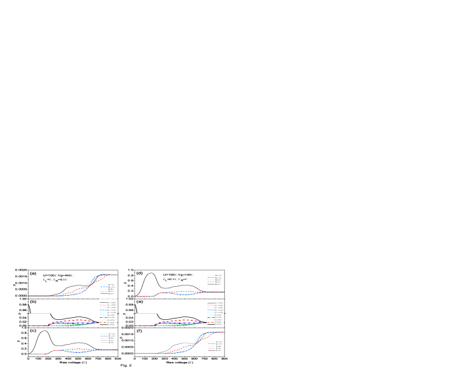
Figure 2: (Colour online) The probability distribution of molecular eigenstates versus bias voltage for different gate voltages with $U=100\Gamma$. (a), (b) and (c) $V_{g}=400\Gamma$ and $\Gamma_{L}/\Gamma_{R}=10$, (d), (e) and (f) $V_{g}=100\Gamma$ and $\Gamma_{L}/\Gamma_{R}=0.1$. The molecular parameters are the same as in Fig. 1.

whose numerical results are shown in Fig. 2. It is because of the both symmetries of the effective channel energy levels and the probability distributions that the FCS of transport through the SMM for $\Gamma_{L}/\Gamma_{R}=10$ at $V_{g}=\epsilon_{d}+U/2\pm\Delta V$ represents the same bias-voltage-dependence as that for $\Gamma_{L}/\Gamma_{R}=0.1$ at $V_{g}=\epsilon_{d}+U/2\mp\Delta V$, which are shown in Fig. 1 for a given finite Coulomb interaction $U=100\Gamma$. The transport characteristic should easily be observed experimentally by reversing the bias voltage between the left and right electrodes and tuning the applied gate voltage; but for the case of $U\rightarrow\infty$, this feature will not be observed because the transition processes between doubly-occupied and the singly-occupied states are prohibited.

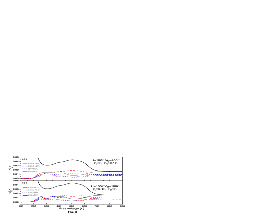
Figure 3: (Colour online) The channel currents versus bias voltage for various gate voltages with $U=100\Gamma$. (a) $V_{g}=400\Gamma$ and $\Gamma_{L}/\Gamma_{R}=10$, (b) $V_{g}=100\Gamma$ and $\Gamma_{L}/\Gamma_{R}=0.1$. The $\left|i\right\rangle\rightarrow\left|j\right\rangle$ denotes the molecular channel current $I_{\left|i\right\rangle\rightarrow\left|j\right\rangle}$. The molecular parameters are the same as in Fig. 1.

It is generally thought that the Coulomb interaction gives rise to the suppression of shot noise[35, 36]. For the present SMM system with finite Coulomb interaction, however, the super-Poissonian shot noise is observed in the sequential tunneling regime. For a given $U=100\Gamma$, as shown in Figs. 1(b) and (e), the super-Poissonian noise for $\Gamma_{L}/\Gamma_{R}=10$ occurs at higher gate voltage such as $V_{g}=300\Gamma$ and $400\Gamma$, while that for $\Gamma_{L}/\Gamma_{R}=0.1$ occurs at lower gate voltage such as $V_{g}=200\Gamma$ and $100\Gamma$, which is consistent with the $U\rightarrow\infty$ case[6]. The presence of the super-Poissonian noise in the sequential tunneling regime can be understood with the help of the dynamic competition between effective fast and slow channels[6, 15, 30, 34, 37, 38, 39]. In order to give a qualitative explanation, we plot the six main molecular channel currents for $V_{g}=400\Gamma$ as a function of bias voltage $V_{b}$ in Fig. 3(a). Here, the calculation of the molecular channel currents can be found in Refs. [5, 6]. When the bias voltage increases up to about $170\Gamma$, the fast channel current $I_{\left|2,2\right\rangle\longrightarrow\left|1,5/2\right\rangle}$ begins to compete with the slow channel currents $I_{\left|2,-2\right\rangle\rightarrow\left|1,-5/2\right\rangle}$, $I_{\left|2,\pm 2\right\rangle\rightarrow\left|1,\pm 3/2\right\rangle^{-}}$ and $I_{\left|2,\pm 1\right\rangle\rightarrow\left|1,\pm 3/2\right\rangle^{-}}$, but the competition is quickly destroyed due to the sum of slow channel currents being approach to the fast channel current, the corresponding noise [the short dashed line in Fig. 1(b)] is only enhanced but does not reach the super-Poissonian. With further increase of the bias voltage (about $250\Gamma$), three sets of the fast-and-slow channel currents are formed, $i.e.$, $I_{\left|2,\pm 2\right\rangle\rightarrow\left|1,\pm 5/2\right\rangle}$ , $I_{\left|2,\pm 2\right\rangle\rightarrow\left|1,\pm 3/2\right\rangle^{-}}$ and $I_{\left|2,\pm 1\right\rangle\rightarrow\left|1,\pm 3/2\right\rangle^{-}}$ , which result in the second enhancement of shot noise. When the bias increases to about $500\Gamma$, the fast channel currents ($I_{\left|2,2\right\rangle\longrightarrow\left|1,5/2\right\rangle}$, $I_{\left|2,2\right\rangle\rightarrow\left|1,3/2\right\rangle^{-}}$ and $I_{\left|2,1\right\rangle\rightarrow\left|1,3/2\right\rangle^{-}}$) begin to decrease, while the corresponding slow channel currents ($I_{\left|2,-2\right\rangle\longrightarrow\left|1,-5/2\right\rangle}$, $I_{\left|2,-2\right\rangle\rightarrow\left|1,-3/2\right\rangle^{-}}$ and $I_{\left|2,-1\right\rangle\rightarrow\left|1,-3/2\right\rangle^{-}}$) begin to increase. The competition between the increase of the slow channel currents and the decrease of the fast channel currents finally leads to appearing of super-Poissonian Fano factor in the bias from about $500\Gamma$ to $625\Gamma$ [the short dashed line in Fig. 1(b)]. Furthermore, we also observe that the super-Poissonian distribution of the skewness $F_{3}$ in the sequential tunneling regime [Fig. 1(c)], which seems sensitive only to the competition between the fast channels of current decreasing and the slow channels of current increasing [Fig. 3(a)]. As for $\Gamma_{L}/\Gamma_{R}=0.1$ at lower gate voltage, the mechanism of shot-noise enhancement originates from the same reason but the effective fast-and-slow transport channels consist of the transitions from the singly-occupied states to empty states, see Fig. 3(b). Furthermore, in the Coulomb blockade regime (see Fig. 1), the shot noise enhancement, as explained in Ref. [34], is due to the possible thermal occupation and subsequent sequential depletion of excited states that lead to small cascades of tunneling events interrupted by long Coulomb blockages. In fact, since in the Coulomb blockade regime the current is exponentially suppressed and the electron transport is dominated by cotunneling, when taking into account cotunneling the normalized second and third moments will deviate from the results obtained by only sequential tunneling[40].

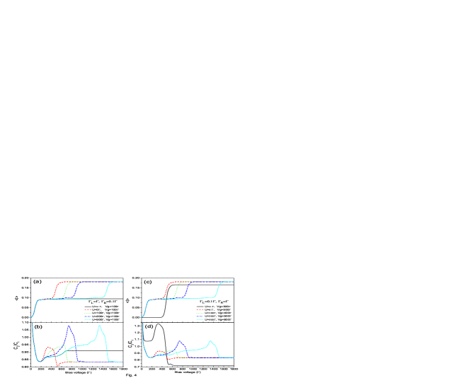
Figure 4: (Colour online) The average current and shot noise versus bias voltage for the different Coulomb interaction energies. (a) and (b) for $\Gamma_{L}/\Gamma_{R}=10$, (c) and (d) for $\Gamma_{L}/\Gamma_{R}=0.1$. The molecular parameters are the same as in Fig. 1.

In contrast with the above case, we find that the finite Coulomb interaction plays a crucial role in determining whether the super-Poissonian noise occurs in situations with relatively small gate voltage for $\Gamma_{L}/\Gamma_{R}>1$ and relatively large gate voltage for $\Gamma_{L}/\Gamma_{R}<1$. In order to study the effects of finite Coulomb interaction on the shot noise in transport through the SMM for the two above-mentioned cases, Fig. 4 shows the current and the shot noise as a function of the bias voltage for various Coulomb interaction energies. For the case of $U\rightarrow\infty$, the super-Poissonian noise, as shown in Figs. 4(b) and (d), dose not appear in the sequential tunneling regime (also see Fig. 2 in Ref. [6]). Here, for the case of $\Gamma_{L}/\Gamma_{R}=0.1$, $U\rightarrow\infty$ and $V_{g}=300\Gamma$, it should be noted that the super-Poissonian noise occurs in the Coulomb blockade regime, see the solid line in Fig. 4(d). Comparing with the $U\rightarrow\infty$ case, the finite Coulomb interaction may induce the super-Poissonian noise only when it is larger than a certain value. We take the case of $V_{g}=100\Gamma$ and $\Gamma_{L}/\Gamma_{R}=10$ for illustration. For small Coulomb interaction (for example, $U=100\Gamma$) the super-Poissonian shot noise does not appear while for relatively larger Coulomb interaction (for example, $U\gtrsim 200\Gamma$) the super-Poissonian shot noise is observed [see Fig. 4(b)]. The role of Coulomb interaction in enhancing shot noise can be understood with the help of the main channel currents shown in Fig. 5. The currents in Figs. 5(a) and (c) result from the electron transitions from singly occupied to empty states while Figs. (b) and (d) correspond to the transitions from doubly occupied to singly occupied states. For small Coulomb interaction $U=100\Gamma$, when the bias changes from $200\Gamma$ to $500\Gamma$ the competition between the fast channel current ($I_{\left|1,5/2\right\rangle\longrightarrow\left|0,2\right\rangle})$ and the slow channel currents ($I_{\left|1,-5/2\right\rangle\longrightarrow\left|0,-2\right\rangle}$, $I_{\left|1,\pm 3/2\right\rangle^{-}\longrightarrow\left|0,\pm 2\right\rangle}$ and $I_{\left|1,\pm 3/2\right\rangle^{-}\longrightarrow\left|0,\pm 1\right\rangle}$) is an active competition in which the increase (or decrease) of the fast channel current is always accompanied by the decrease (or increase) of the slow channel currents, which makes the shot noise increase from 0.84 to 0.93 [see Fig. 4(b)]. With the bias approaching to $600\Gamma$ the currents $I_{\left|2,2\right\rangle\longrightarrow\left|1,5/2\right\rangle}$ and $I_{\left|2,2\right\rangle\longrightarrow\left|1,3/2\right\rangle^{\pm}}$ begin to compete with $I_{\left|1,5/2\right\rangle\longrightarrow\left|0,2\right\rangle}$, but the rapid increase of the amplitudes of $I_{\left|2,2\right\rangle\longrightarrow\left|1,5/2\right\rangle}$ and $I_{\left|2,2\right\rangle\longrightarrow\left|1,3/2\right\rangle^{\pm}}$ lead to rapid decrease of $I_{\left|1,5/2\right\rangle\longrightarrow\left|0,2\right\rangle}$ and even destroy the competition, as a result the shot noise quickly drops to sub-Poissonian after increasing to 0.95 near $V_{b}=640\Gamma$[see fig. 4(b)]. When Coulomb interaction increases to $200\Gamma$, the bias voltage regime in which the active competition occurs is much larger than that for $U=100\Gamma$, $i.e.$, from $200\Gamma$ to $750\Gamma$ [see Fig. 5(c)], so that the shot noise has reached super-Poissonian before the effective competition between the fast and slow channels is destroyed by the rapid rise of $I_{\left|2,2\right\rangle\longrightarrow\left|1,5/2\right\rangle}$ and $I_{\left|2,2\right\rangle\longrightarrow\left|1,3/2\right\rangle^{\pm}}$ [see Figs. 5(c) and (d)].

On the other hand, although the shot noise of finite Coulomb interaction for $\Gamma_{L}/\Gamma_{R}=0.1$ in Fig. 4(d) have the same bias-voltage-dependence as that for $\Gamma_{L}/\Gamma_{R}=10$ in Fig. 4(b), the corresponding transport processes are different due to occurring at different gate voltages, which may be found by comparing the main channel currents in Fig. 6(a) (for $\Gamma_{L}/\Gamma_{R}=0.1$, $U=100\Gamma$ and $V_{g}=400\Gamma$) with those in Figs. 5(a) and (b) (for $\Gamma_{L}/\Gamma_{R}=10,$ $U=100\Gamma$ and $V_{g}=100\Gamma$). In particular, for the case of $\Gamma_{L}/\Gamma_{R}=0.1,$ $U=100\Gamma$ and $V_{g}=400\Gamma$ there is a reverse current $I_{\left|0,2\right\rangle\longrightarrow\left|1,5/2\right\rangle}$ near $V_{b}=600\Gamma$ besides a rapidly increasing current $I_{\left|1,5/2\right\rangle\longrightarrow\left|0,2\right\rangle}$ [see Fig. 6(a)] and the two currents destroy the competition between the fast and slow channels, resulting in rapid decrease of the shot noise. For the case of $U=200\Gamma$ and $V_{g}=500\Gamma$, as shown in Fig. 6(b), the bias voltage regime in which the active competition occurs is much larger than that for $U=100\Gamma$ and $V_{g}=400\Gamma,$ $i.e.,$ from $200\Gamma$ to $750\Gamma$ (it is from $200\Gamma$ to $640\Gamma$ for $U=100\Gamma$ and $V_{g}=400\Gamma$), so that the shot noise has reached super-Poissonian before the reverse current and the rapidly increasing current occur. As a result the shot noise rapidly drops from the super-Poissonian to the sub-Poissonian.

The theoretical investigations have predicted that the super-Poissonian noise may occur in the quantum dot systems[38, 39, 40] and molecular junction[13] coupled symmetrically to two electrodes. For the present SMM system, when it symmetrically couples to two leads the super-Poissonian noise in the sequential tunneling regime is observed only under an appropriate finite Coulomb interaction that determined by the parameters of the SMM (see Fig. 7), which still not appears in the case of $U=0$ and $U\rightarrow\infty$. The noise characteristics can still be attributed to the competition between the effective fast and slow transport channels.

4 Conclusions

We have studied the effect of finite Coulomb interaction on the FCS of electron transport through a SMM weakly coupled to two metallic electrodes above the sequential tunneling threshold by means of the particle-number-resolved quantum master equation. The electron transport through the SMM with finite Coulomb interaction $U$ has richer current correlation due to the transitions of doubly-occupied to singly-occupied states participating in transport. Compared with the $U\rightarrow\infty$ case, our analytical results show that the finite Coulomb interaction induces that the effective channel energy levels move symmetrically into the bias voltage window with increasing the bias voltage, as a result the FCS for $V_{g}=\epsilon_{d}+U/2\pm\Delta V$ has the same bias-voltage-dependence as that for $V_{g}=\epsilon_{d}+U/2\mp\Delta V$ (i.e., the FCS shows the symmetrical gate-voltage-dependence) when both the intensities of the SMM coupling to the left and right electrodes are interchanged, which should easily be observed experimentally by reversing the bias voltage. Moreover, we find that the effect of finite Coulomb interaction on the shot noise depends not only on the gate voltage, but also on the left-right asymmetry of SMM-electrode couplings. In the case of $\Gamma_{L}/\Gamma_{R}>1$, for an arbitrary given $U$ (which contains $U=0$ and $U\rightarrow\infty$) the super-Poissonian shot noise in the sequential tunneling regime may be observed at a relatively large gate voltage; whereas at a relatively small gate voltage the super-Poissonian shot noise does not occur for the cases of $U=0$ and $U\rightarrow\infty$, and may appear only when $U$ is the finite value which is related to the parameters of the SMM. For the $\Gamma_{L}/\Gamma_{R}<1$ case, the super-Poissonian shot noise is found at a relatively small gate voltage for an arbitrary given $U$; whereas at a relatively large gate voltage it may occur only for a relatively large finite Coulomb interaction, which is contrary to the $\Gamma_{L}/\Gamma_{R}>1$ case. These characteristics of shot noise can be understood as a result of the active competition between the fast and slow channel currents.

Appendix

In this appendix, we take $\left\langle 1,-\frac{5}{2}\right|S\left(\chi,t\right)\left|1,-\frac{5}{2}\right\rangle$ as an example to illustrate the procedure for obtaining the specific form of $\mathcal{L}_{\chi}$. Based on the $S\left(\chi,t\right)$ definition and Eq. (11), after a careful calculation, the equation of motion for $\left\langle 1,-\frac{5}{2}\right|S\left(\chi,t\right)\left|1,-\frac{5}{2}\right\rangle$ is given by

$$\left\langle 1,-\frac{5}{2}\right|\overset{\cdot}{S}\left(\chi,t\right)\left|1,-\frac{5}{2}\right\rangle$$ (A.1)

$$= -\Gamma_{L}n_{L}^{\left(+\right)}\left(\epsilon_{\left|2,-2\right\rangle}-\epsilon_{\left|1,-\frac{5}{2}\right\rangle}\right)\left\langle 1,-\frac{5}{2}\right|S\left|1,-\frac{5}{2}\right\rangle$$

$$-\Gamma_{R}n_{R}^{\left(+\right)}\left(\epsilon_{\left|2,-2\right\rangle}-\epsilon_{\left|1,-\frac{5}{2}\right\rangle}\right)\left\langle 1,-\frac{5}{2}\right|S\left|1,-\frac{5}{2}\right\rangle$$

$$-\Gamma_{L}n_{L}^{\left(-\right)}\left(\epsilon_{\left|1,-\frac{5}{2}\right\rangle}-\epsilon_{\left|0,-2\right\rangle}\right)\left\langle 1,-\frac{5}{2}\right|S\left|1,-\frac{5}{2}\right\rangle$$

$$-\Gamma_{R}n_{R}^{\left(-\right)}\left(\epsilon_{\left|1,-\frac{5}{2}\right\rangle}-\epsilon_{\left|0,-2\right\rangle}\right)\left\langle 1,-\frac{5}{2}\right|S\left|1,-\frac{5}{2}\right\rangle$$

$$+\Gamma_{L}n_{L}^{\left(-\right)}\left(\epsilon_{\left|2,-2\right\rangle}-\epsilon_{\left|1,-\frac{5}{2}\right\rangle}\right)\left\langle 2,-2\right|S\left|2,-2\right\rangle$$

$$+\Gamma_{R}n_{R}^{\left(-\right)}\left(\epsilon_{\left|2,-2\right\rangle}-\epsilon_{\left|1,-\frac{5}{2}\right\rangle}\right)e^{i\chi}\left\langle 2,-2\right|S\left|2,-2\right\rangle$$

$$+\Gamma_{L}n_{L}^{\left(+\right)}\left(\epsilon_{\left|1,-\frac{5}{2}\right\rangle}-\epsilon_{\left|0,-2\right\rangle}\right)\left\langle 0,-2\right|S\left|0,-2\right\rangle$$

$$+\Gamma_{R}n_{R}^{\left(+\right)}\left(\epsilon_{\left|1,-\frac{5}{2}\right\rangle}-\epsilon_{\left|0,-2\right\rangle}\right)e^{-i\chi}\left\langle 0,-2\right|S\left|0,-2\right\rangle.$$

Similarly, we can carry out the equations of motion for other matrix elements, which can be rewritten as a compact matrix form

$$\mathcal{\dot{S}}=\mathcal{L}_{\chi}\mathcal{S}.$$ (A.2)

Here, the column matrix $\mathcal{S}$ has the following form

$$\mathcal{S} = \left[\left\langle 1,-\frac{5}{2}\right|S\left|1,-\frac{5}{2}\right\rangle,\left\langle 2,-2\right|S\left|2,-2\right\rangle,\right.$$ (A.3)

$$\left.\left\langle 0,-2\right|S\left|0,-2\right\rangle,^{+}\left\langle 1,-\frac{3}{2}\right|S\left|1,-\frac{3}{2}\right\rangle^{+},^{+}\left\langle 1,-\frac{3}{2}\right|S\left|1,-\frac{3}{2}\right\rangle^{-},\right.$$

$$\left.{}^{-}\left\langle 1,-\frac{3}{2}\right|S\left|1,-\frac{3}{2}\right\rangle^{+},^{-}\left\langle 1,-\frac{3}{2}\right|S\left|1,-\frac{3}{2}\right\rangle^{-},\left\langle 2,-1\right|S\left|2,-1\right\rangle,\right.$$

$$\left.\left\langle 0,-1\right|S\left|0,-1\right\rangle,^{+}\left\langle 1,-\frac{1}{2}\right|S\left|1,-\frac{1}{2}\right\rangle^{+},^{+}\left\langle 1,-\frac{1}{2}\right|S\left|1,-\frac{1}{2}\right\rangle^{-},\right.$$

$$\left.{}^{-}\left\langle 1,-\frac{1}{2}\right|S\left|1,-\frac{1}{2}\right\rangle^{+},^{-}\left\langle 1,-\frac{1}{2}\right|S\left|1,-\frac{1}{2}\right\rangle^{-},\left\langle 2,0\right|S\left|2,0\right\rangle,\right.$$

$$\left.\left\langle 0,0\right|S\left|0,0\right\rangle,^{+}\left\langle 1,\frac{1}{2}\right|S\left|1,\frac{1}{2}\right\rangle^{+},^{+}\left\langle 1,\frac{1}{2}\right|S\left|1,\frac{1}{2}\right\rangle^{-},\right.$$

$$\left.{}^{-}\left\langle 1,\frac{1}{2}\right|S\left|1,\frac{1}{2}\right\rangle^{+},^{-}\left\langle 1,\frac{1}{2}\right|S\left|1,\frac{1}{2}\right\rangle^{-},\left\langle 2,1\right|S\left|2,1\right\rangle,\right.$$

$$\left.\left\langle 0,1\right|S\left|0,1\right\rangle,^{+}\left\langle 1,\frac{3}{2}\right|S\left|1,\frac{3}{2}\right\rangle^{+},^{+}\left\langle 1,\frac{3}{2}\right|S\left|1,\frac{3}{2}\right\rangle^{-},\right.$$

$$\left.{}^{-}\left\langle 1,\frac{3}{2}\right|S\left|1,\frac{3}{2}\right\rangle^{+},^{-}\left\langle 1,\frac{3}{2}\right|S\left|1,\frac{3}{2}\right\rangle^{-},\left\langle 2,2\right|S\left|2,2\right\rangle,\right.$$

$$\left.\left\langle 0,2\right|S\left|0,2\right\rangle,\left\langle 1,\frac{5}{2}\right|S\left|1,\frac{5}{2}\right\rangle\right]^{T}.$$

From Eq. (A.1), the first row of $\mathcal{L}_{\chi}$ is given by

$$\left[{\mathcal{L}_{\chi}}\right]_{1\times 28} = \left[\left[{\mathcal{L}_{\chi}}\right]_{1,1},\right.$$ (A.4)

$$\left.\left[{\mathcal{L}_{\chi}}\right]_{1,2},\left[{\mathcal{L}_{\chi}}\right]_{1,3},0,0,0,0,0,0,\right.$$

$$\left.0,0,0,0,0,0,0,0,\right.$$

$$\left.0,0,0,0,0,0,0,0,\right.$$

$$\left.0,0,0\right]$$

with

$$\left[{\mathcal{L}_{\chi}}\right]_{1,1} = -\Gamma_{L}n_{L}^{\left(+\right)}\left(\epsilon_{\left|2,-2\right\rangle}-\epsilon_{\left|1,-\frac{5}{2}\right\rangle}\right)-\Gamma_{R}n_{R}^{\left(+\right)}\left(\epsilon_{\left|2,-2\right\rangle}-\epsilon_{\left|1,-\frac{5}{2}\right\rangle}\right)$$

$$-\Gamma_{L}n_{L}^{\left(-\right)}\left(\epsilon_{\left|1,-\frac{5}{2}\right\rangle}-\epsilon_{\left|0,-2\right\rangle}\right)-\Gamma_{R}n_{R}^{\left(-\right)}\left(\epsilon_{\left|1,-\frac{5}{2}\right\rangle}-\epsilon_{\left|0,-2\right\rangle}\right),$$

$$\left[{\mathcal{L}_{\chi}}\right]_{1,2}=\Gamma_{L}n_{L}^{\left(-\right)}\left(\epsilon_{\left|2,-2\right\rangle}-\epsilon_{\left|1,-\frac{5}{2}\right\rangle}\right)+\Gamma_{R}n_{R}^{\left(-\right)}\left(\epsilon_{\left|2,-2\right\rangle}-\epsilon_{\left|1,-\frac{5}{2}\right\rangle}\right)e^{i\chi},$$

$$\left[{\mathcal{L}_{\chi}}\right]_{1,3}=\Gamma_{L}n_{L}^{\left(+\right)}\left(\epsilon_{\left|1,-\frac{5}{2}\right\rangle}-\epsilon_{\left|0,-2\right\rangle}\right)+\Gamma_{R}n_{R}^{\left(+\right)}\left(\epsilon_{\left|1,-\frac{5}{2}\right\rangle}-\epsilon_{\left|0,-2\right\rangle}\right)e^{-i\chi}.$$

Figure 1: (Colour online) The first three cumulants of zero-frequency current fluctuation versus bias voltage for different gate voltages. (a), (b) and (c) for $\Gamma_{L}/\Gamma_{R}=10$, (d), (e) and (f) for $\Gamma_{L}/\Gamma_{R}=0.1$. The molecular parameters: $S=2$, $\varepsilon_{d}=200\Gamma$, $J=100\Gamma$, $K_{2}=40\Gamma$, $B=80\Gamma$ and $k_{B}T=10\Gamma$.

Figure 5: (Colour online) The channel currents versus bias voltage for different Coulomb interaction energies with $\Gamma_{L}/\Gamma_{R}=10$. (a) and (b) $U=100\Gamma$, $V_{g}=100\Gamma$, (c) and (d) $U=200\Gamma$, $V_{g}=100\Gamma$. The channel current expression and molecular parameters are the same as Fig. 3.

Figure 6: (Colour online) The channel currents versus bias voltage for different Coulomb interaction energies with $\Gamma_{L}/\Gamma_{R}=0.1$. (a) for $U=100\Gamma$, $V_{g}=400\Gamma$, (b) $U=200\Gamma$, $V_{g}=500\Gamma$. The channel current expression and molecular parameters are the same as Fig. 3.

Figure 7: (Colour online) The average current and shot noise versus bias voltage for different Coulomb interaction energies with $\Gamma_{L}=\Gamma_{R}=\Gamma$. The molecular parameters are the same as in Fig. 1.

References

- [1] H.B. Heersche, Z. de Groot, J.A. Folk, H.S.J. van der Zant, C. Romeike, M.R. Wegewijs, L.Zobbi, D. Barreca, E. Tondello, A. Cornia, Phys. Rev. Lett. 96 (2006) 206801; Moon-Ho Jo, J.E. Grose, K. Baheti, M.M. Deshmukh, J.J. Sokol, E.M. Rumberger, D.N. Hendrickson, J.R. Long, H. Park, D.C. Ralph, Nano Lett. 6 (2006) 2014; J.E. Grose, E.S. Tam, C. Timm, M. Scheloske, B. Ulgut, J.J. Parks, H.D. Abruna, W. Harneit, D.C. Ralph, Nature Mat. 7 (2008) 884.
- [2] C. Romeike, M.R. Wegewijs, W. Hofstetter, H. Schoeller, Phys. Rev. Lett. 96 (2006) 196601; C. Romeike, M.R. Wegewijs, W. Hofstetter, H. Schoeller, Phys. Rev. Lett. 97 (2006) 206601.
- [3] C. Romeike, M.R. Wegewijs, H. Schoeller, Phys. Rev. Lett. 96 (2006) 196805.
- [4] F. Elste, C. Timm, Phys. Rev. B 71, 155403 (2005); F. Elste, F. von Oppen, New J. Phys. 10 (2008) 065021; F. Elste, G. Weick, C. Timm, F. von Oppen, Appl. Phys. A 93 (2008) 345.
- [5] C. Timm, F. Elste, Phys. Rev. B 73 (2006) 235304; F. Elste, C. Timm, Phys. Rev. B 73 (2006) 235305; F. Elste, C. Timm, Phys. Rev. B 75 (2007) 195341; C. Timm, Phys. Rev. B 76 (2007) 014421.
- [6] Hai-Bin Xue, Y.-H. Nie, Z.-J. Li, J.-Q. Liang, J. Appl. Phys. 108 (2010) 033707.
- [7] M.N. Leuenberger, E.R. Mucciolo, Phys. Rev. Lett. 97 (2006) 126601; G. González, M.N. Leuenberger, Phys. Rev. Lett. 98 (2007) 256804; G. González, M.N. Leuenberger, E.R. Mucciolo, Phys. Rev. B 78 (2008) 054445.
- [8] M. Misiorny, J. Barnaś, Phys. Rev. B 75 (2007) 134425 ; ibid 76 (2007) 054448; ibid 77 (2008) 172414; M. Misiorny, J. Barnaś, Europhys. Lett. 78 (2007) 27003.
- [9] H.-Z. Lu, B. Zhou, and S.-Q. Shen, Phys. Rev. B 79 (2009) 174419.
- [10] B. Lapo, W. Wolfgang, Nature Mat. 7 (2008) 179.
- [11] D. Djukic, J.M. van Ruitenbeek, Nano Lett. 6 (2006) 789.
- [12] K.-I. Imura, Y. Utsumi, T. Martin, Phys. Rev. B 75 (2007) 205341.
- [13] S. Welack, J.B. Maddox, M. Esposito, U. Harbola, S. Mukamel, Nano Lett. 8 (2008) 1137.
- [14] B. Dong, H.Y. Fan, X.L. Lei, N.J.M. Horing, J. Appl. Phys. 105 (2009) 113702.
- [15] L. D. Contreras-Pulido and R. Aguado, Phys. Rev. B 81 (2010) 161309.
- [16] W. Belzig, Phys. Rev. B 71 (2005) 161301(R).
- [17] Ya.M. Blanter, M. Büttiker, Phys. Rep. 336 (2000) 1; Quantum Noise in Mesoscopic Physics, edited by Yu.V. Nazarov Kluwer, Dordrecht, 2003.
- [18] L.Y. Chen, C.S. Ting, Phys. Rev. B 43 (1991) 4534; M. Büttiker, Physica B 175 (1991) 199.
- [19] T. González, C. González, J. Mateos, D. Pardo, L. Reggiani, O.M. Bulashenko, J.M. Rubí, Phys. Rev. Lett. 80 (1998) 2901.
- [20] G. Iannaccone, G. Lombardi, M. Macucci, B. Pellegrini, Phys. Rev. Lett. 80 (1998) 1054.
- [21] A. Reklaitis, L. Reggiani, Phys. Rev. B 62 (2000) 16773 ; Physica B 272 (1999) 279.
- [22] A.V. Galaktionov, D.S. Golubev, A.D. Zaikin, Phys. Rev. B 68 (2003) 085317.
- [23] E. Sela, Y. Oreg, F. von Oppen, J. Koch, Phys. Rev. Lett. 97 (2006) 086601.
- [24] A. Golub, Phys. Rev. B 75 (2007) 155313.
- [25] M. Naspreda, O.M. Bulashenko, J.M. Rubí, Phys. Rev. B 68 (2003) 155321.
- [26] L.S. Levitov, H.-W. Lee, G.B. Lesovik, J. Math. Phys. 37 (1996) 4845.
- [27] D.A. Bagrets, Yu.V. Nazarov, Phys. Rev. B 67 (2003) 085316.
- [28] X.-Q. Li, P. Cui, Y.J. Yan, Phys. Rev. Lett. 94 (2005) 066803.
- [29] X.-Q. Li, J. Luo, Y.-G. Yang, P. Cui, Y.J. Yan, Phys. Rev. B 71 (2005) 205304.
- [30] S.-K. Wang, H. Jiao, F. Li, X.-Q. Li, Y.J. Yan, Phys. Rev. B 76 (2007) 125416.
- [31] C.W. Groth, B. Michaelis, C.W.J. Beenakker, Phys. Rev. B 74 (2006) 125315; C. Flindt, T. Novotny, A.P. Jauho, Europhys. Lett. 69 (2005) 475; G. Kießlich, P. Samuelsson, A. Wacker, E. Schöll, Phys. Rev. B 73 (2006) 033312.
- [32] A. Morello, O.N. Bakharev, H.B. Brom, R. Sessoli, L.J. de Jongh, Phys. Rev. Lett. 93 (2004) 197202; A. Ardavan, O. Rival, J.J.L. Morton, S.J. Blundell, A.M. Tyryshkin, G.A. Timco, R.E.P. Winpenny, ibid. 98 (2007) 057201; S. Bahr, K. Petukhov, V. Mosser, W. Wernsdorfer, ibid. 99 (2007) 147205.
- [33] H. Park, J. Park, A.K.L. Lim, E.H. Anderson, A.P. Alivisatos, P.L. McEuen, Nature 407 (2000) 57; J. Park, A.N. Pasupathy, J.I. Goldsmith, C. Chang, Y. Yaish, J.R. Petta, M. Rinkoski, J.P. Sethna, H.D. Abruña, P.L. McEuen, D.C. Ralph, ibid 417 (2002) 722.
- [34] J. Aghassi, A. Thielmann, M.H. Hettler, G. Schön, Phys. Rev. B 73 (2006) 195323.
- [35] M. Reznikov, M. Heiblum, H. Shtrikman, D. Mahalu, Phys. Rev. Lett. 75 (1995) 3340.
- [36] M. Hamasaki, Phys. Rev. B 69 (2004) 115313.
- [37] S.S. Safonov, A.K. Savchenko, D.A. Bagrets, O.N. Jouravlev, Yu.V. Nazarov, E.H. Linfield, D.A. Ritchie, Phys. Rev. Lett. 91 (2003) 136801.
- [38] I. Djuric, B. Dong, H.L. Cui, Appl. Phys. Lett. 87 (2005) 032105.
- [39] J. Aghassia, A. Thielmann, M.H. Hettler, G. Schön, Appl. Phys. Lett. 89 (2006) 052101.
- [40] A. Thielmann, M.H. Hettler, J. König, G. Schön, Phys. Rev. Lett. 95 (2005) 146806.