Future CMB Constraints on Early, Cold, or Stressed Dark Energy

Abstract

We investigate future constraints on early dark energy (EDE) achievable by the Planck and CMBPol experiments, including cosmic microwave background (CMB) lensing. For the dark energy, we include the possibility of clustering through a sound speed $c_{\rm s}^{2}<1$ (cold dark energy) and anisotropic stresses parameterized with a viscosity parameter $c_{\rm vis}^{2}$. We discuss the degeneracies between cosmological parameters and EDE parameters. In particular we show that the presence of anisotropic stresses in EDE models can substantially undermine the determination of the EDE sound speed parameter $c_{\rm s}^{2}$. The constraints on EDE primordial energy density are however unaffected. We also calculate the future CMB constraints on neutrino masses and find that they are weakened by a factor of 2 when allowing for the presence of EDE, and highly biased if it is incorrectly ignored.

I Introduction

For about a decade cosmological data from cosmic microwave background (CMB) anisotropy experiments (wmap7 , acbar , quad ), in combination with complementary results from galaxy surveys 2dF ; SDSS and Type Ia supernovae PerlRiess ; union2 , suggest in an unequivocable way that the present energy budget of the universe is dominated by an exotic form of energy coined dark energy.

The presence of a cosmological constant term $\Lambda$ in Einstein’s equation of General Relativity (GR) is the simplest explanation for dark energy. The Lambda cold dark matter scenario ($\Lambda$CDM) is a simple model that consistently accounts for all observations, and has therefore emerged as the standard model of cosmology. Despite the simplicity of this concordance model, however, the presence of a tiny but nonzero cosmological constant is vexing, and is not understood from the point of view of fundamental theory (see e.g. lambda and references therein). Dark energy could therefore be different from a cosmological constant, and indeed many diverse models are also consistent with the data beylam ; sollerman ; mhh2 .

Within the framework of a non-interacting, minimally coupled additional component to the energy density, a general dark energy fluid and the cosmological constant may differ in two main aspects: the latter behaves as a homogeneous fluid with a constant energy density, while the former is a non-homogeneous fluid with a time dependent energy density and pressure. A simple way of describing these models is by specifying the equation of state $w=p/\rho$, where $p$ and $\rho$ are the dark energy pressure and density. The cosmological constant corresponds to $w=-1$, while a general dark energy fluid may have a time dependent equation of state $w(a)$ which is as function of the scale factor $a(t)$, so that $w\neq-1$ in general.

Density perturbations in the dark energy component could also leave an imprint in cosmological observables, while $\Lambda$ is purely homogeneous. The clustering properties of different dark energy models are usually parameterized by an effective sound speed, defined as the ratio between the pressure to density perturbations in the rest frame of dark energy; $c_{\rm s}^{2}=\delta p/\delta\rho$ (see, e.g., Hu98 ; Bean ; JochenLewis ). Moreover, anisotropic stress can also affect the density perturbations. For example, in the case of a relativistic component, anisotropic stresses act as a form of viscosity in the fluid and damp density pertubations. If dark energy behaves like a relativistic fluid in the past, then the effects of viscosity should also be considered.

To parameterize viscosity in a dark component one can introduce the viscous sound speed $c_{\rm vis}^{2}$, which controls the relationship between velocity/metric shear and the anisotropic stress Hu98 ; Koivisto:2008ig ; mota . A value of $c_{\rm vis}^{2}=1/3$, for example, is what one expects for a relativistic component, where anisotropic stress is present and approximates the radiative viscosity of a relativistic fluid. The standard assumption is that $c_{\rm vis}^{2}=0$, which however cuts the Boltzmann hierarchy of perturbations at the quadrupole, forcing a perfect fluid solution with only density, velocity and (isotropic) pressure perturbations.

Any indication for perturbations in the dark energy fluid would falsify a scenario based on the cosmological constant. However, since perturbations become observationally unimportant as the equation of state approaches the cosmological constant value, $w=-1$, to detect them one needs some period in cosmic history when $w$ differs substantially from $-1$. Such a deviation in $w$ is constrained at late times by the observations, so we are led to consider this at early times, along with a non-negligible early dark energy density.

Such early dark energy can arise in some cases of the tracking class of dark energy models (see, e.g., tracking ). In particular, in tracing models the dark energy density is a constant fraction of the dominant component, radiation or matter. If this fraction is non-negligible, dark energy could therefore be appreciable not only in the late universe but also at early times. Several models of “early” dark energy (EDE, hereafter) have been proposed (e.g. Doran:2006kp ; Linder:2006da and references therein).

Our paper is organized as follows: in Section II we discuss the EDE model and the behaviour of perturbations. In Section III we explain the types of CMB data used and the forecast method, including the weak lensing signal. In Section IV we present our results, and finally in Section V we discuss our conclusions.

II Early Dark Energy

II.1 Model

In Doran:2006kp a parametrization for the dark energy density parameter $\Omega_{\rm de}(a)$ and equation of state $w(a)$ has been proposed to recognize the important feature of early dark energy. In this model $\Omega_{\rm de}^{0}$ and $\Omega_{m}^{0}$ are the current dark energy and matter density, respectively, and a flat Universe is assumed so $\Omega_{m}^{0}+\Omega_{\rm de}^{0}=1$. The model is described by :

$$\Omega_{\rm de}(a) = \frac{\Omega_{\rm de}^{0}-\Omega_{\rm e}\left(1-a^{-3w_{0}}\right)}{\Omega_{\rm de}^{0}+\Omega_{m}^{0}a^{3w_{0}}}+\Omega_{\rm e}\left(1-a^{-3w_{0}}\right)$$ (1)

$$w(a) = -\frac{1}{3[1-\Omega_{\rm de}(a)]}\frac{d\ln\Omega_{\rm de}(a)}{d\ln a}+\frac{a_{eq}}{3(a+a_{eq})}$$ (2)

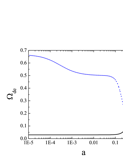
where $\Omega_{\rm e}$ is the early dark energy component density, constant at high redshift, $a_{eq}$ is the scale factor at matter-radiation equality, and $w_{0}=w(a=1)$. In Figure 1 we plot $\Omega_{\rm de}(a)$ and $w(a)$, for $w_{0}=-1$, $\Omega_{\rm e}=0.03$ and $\Omega_{\rm de}^{0}=0.7$. Note the energy density $\Omega_{\rm de}(a)$ goes to a nonnegligible constant in the past (whereas $\Omega_{\Lambda}(a=10^{-3})\approx 10^{-9}$). The dark energy equation of state $w(a)$ clearly shows $3$ different behaviours: $w\sim 1/3$ during the radiation dominated era, $w\sim 0$ during matter domination and, finally, $w\sim w_{0}$ in recent epochs.

Figure 1: Behaviour of the early dark energy model in energy density (solid black line) and equation of state (dotted blue line) as a function of the scale factor.

Moreover such an EDE model with constant sound speed can behave like barotropic dark energy models (see e.g. Linder:2008ya , and Fig. 2 of dePutter:2010vy ). These models have an explicit relation determining the pressure as a function of energy density that bring advantages to overcome the coincidence problem and to predict a value of $w_{0}\approx-1$ at late times, considering purely physical properties rather than being adopted as phenomenology.

Recent analyses have placed constraints on EDE using the available cosmological datasets and forecasting the discriminatory power of future CMB probes such as Planck (see e.g. dePutter:2010vy ; Alam:2010tt ; Hollenstein:2009ph ; Xia:2009ys ). As recently shown in particular, the effects of EDE could be important when combining CMB data with baryonic acoustic oscillation data linderbao . In this paper we follow the lines of these recent papers and we present a forecast for EDE parameters from the near future Planck planck and far future CMBPol Bock:2009xw experiments. Our work will improve similar recent analyses in several aspects. First, we consider the possibility of perturbations in EDE including an anisotropic stress term in EDE, parametrized by a viscosity sound speed $c_{\rm vis}$ (see Hu98 ). If EDE is following an equation of state of a relativistic fluid, anisotropic stresses can be present and change in a substantial way the theoretical predictions on the CMB angular spectrum. Secondly, we include the CMB weak lensing signal, discussing its importance in constraining EDE parameters. Finally we also tested our results performing a full Monte Carlo Markov Chain (MCMC) on Planck synthetic dataset.

II.2 Perturbation theory

Here we briefly review the perturbations in EDE and show theoretical predictions for the CMB anisotropy angular spectra and for the weak lensing CMB signal.

In the synchronous gauge, the energy-momentum conservation in the Fourier space gives the following equations for the evolution of the density and velocity perturbations (see Hu98 , Ma ) :

$$\frac{\dot{\delta}}{1+w} = -\left[k^{2}+9\left(\frac{\dot{a}}{a}\right)^{2}\left(c_{\rm s}^{2}-w+\frac{\dot{w}}{3(1+w)(\dot{a}/a)}\right)\right]\frac{\theta}{k^{2}}$$ (3)

$$-\frac{\dot{h}}{2}-3\frac{\dot{a}}{a}(c_{\rm s}^{2}-w)\frac{\delta}{1+w}$$

$$\dot{\theta} = -\frac{\dot{a}}{a}(1-3c_{\rm s}^{2})\,\theta+\frac{\delta}{1+w}c_{\rm s}^{2}k^{2}-k^{2}\sigma$$ (4)

$$\dot{\sigma} = -3\frac{\dot{a}}{a}\left[1-\frac{\dot{w}}{3w(1+w)(\dot{a}/a)}\right]\,\sigma$$ (5)

$$+\frac{8c_{\rm vis}^{2}}{3(1+w)}\left[\theta+\frac{\dot{h}}{2}+3\dot{\eta}\right]$$

where $\delta$ and $\theta$ are the dark energy density perturbation and velocity perturbation, $h$ is the metric perturbation source, and $-h/2-3\eta$ is the scalar potential of the tensorial metric perturbations.

The above equations describe various models of dark energy; note that even if $w(a)$ is the same for two models, they can differ in the perturbations. For a chosen model one can implement these relations in a modified version of CAMB camb and solve the Einstein-Boltzmann equations.

III Effects on the CMB

III.1 CMB Angular Spectra

As already discussed in the literature (see e.g. Bean and JochenLewis ), perturbations in a dark energy component with a constant equation of state and a negligible energy component in the early universe (i.e. $\Omega_{e}=0$ and $w(a)=w_{0}$) affect the CMB anisotropy only on very large angular scales, where cosmic variance dominates. The reason is that since in this scenario dark energy contributes appreciable energy density only at late times and is minimally coupled with other energy components, changes in the CMB spectra can be only induced by the late Integrated Sachs-Wolfe (ISW) component.

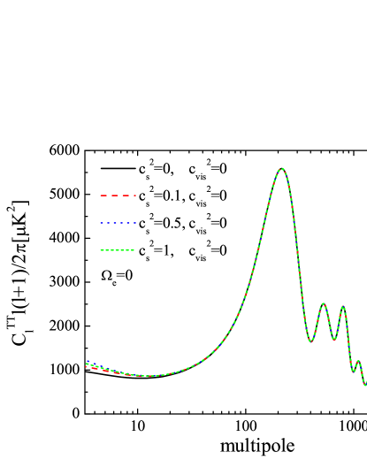
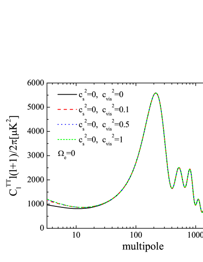
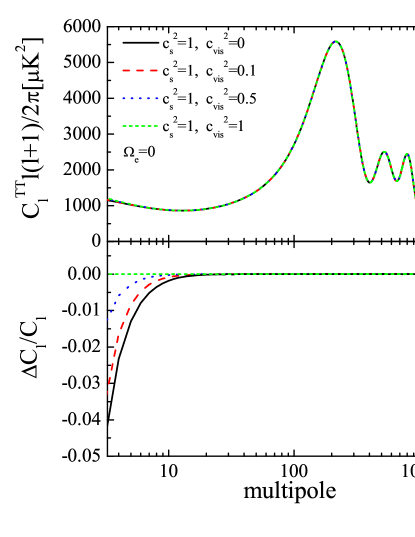
As an example, we plot in Figure 2 the CMB angular spectra for different values of $c_{\rm s}^{2}$ and $c_{\rm vis}^{2}$: the variation is only present on large scales (low multipoles). As already discussed in the literature, the feasibility of accurately measuring one of these parameters is strongly undermined by the presence of cosmic variance. Moreover, the effects of the two parameters are not uncorrelated with each other, as we show in Figure 3. Fixing $c_{\rm vis}^{2}=1$ or $c_{\rm s}^{2}=1$ makes the angular spectra independent of any variation of the other parameter ($c_{\rm s}^{2}$ or $c_{\rm vis}^{2}$, respectively). If one assumes either $c_{\rm vis}^{2}=1$ (shown in the top panel), or $c_{\rm s}^{2}=1$ (bottom panel), one is maximally suppressing the perturbations, giving essentially identical power spectra for different values of $c_{\rm s}^{2}$ or $c_{\rm vis}^{2}$, respectively. This discussion is fully compatible with the results presented in mota .

The net effect of increasing $c_{\rm s}^{2}$ or $c_{\rm vis}^{2}$ is higher ISW power. This reflects the increased potential decay due to dark energy; while dark energy perturbations would help preserve the potential, increasing $c_{\rm s}^{2}$ or $c_{\rm vis}^{2}$ reduces the dark energy perturbation contribution and so eases the decay of the potential. For example, $\Lambda$ leads to a high ISW power today. The effect can be explained more mathematically as follows. The metric perturbation, $h$, is a source term in the density equation (3) and tends to draw dark energy into overdensities of cold dark matter.

However, for positive $c_{s}^{2}$ and/or positive $c^{2}_{vis}$, the term proportional to $\theta$ dominates (on small enough scales) and suppresses perturbations. In the case of positive $c_{s}^{2}$, this can be seen directly from equation (4), where the term proportional to $c_{s}^{2}$ implies that the sign of $\theta$ is the same as that of $\delta$ so that the contribution to $\dot{\delta}$ has the opposite sign of $\delta$, leading to suppression (a comparison of the magnitudes of the different terms shows that the suppression becomes dominant roughly for scales $k>c_{s}^{-1}\left(\dot{a}/a\right)$). Thus $\delta$ gets smaller when dark energy begins to dominate and the ISW effect is enhanced when one increases the sound speed. In the case of positive $c^{2}_{vis}$, it follows from the sign of the metric terms in equation (5) that $\sigma$ ends up with the same sign as $\delta$, again giving a contribution to the $\dot{\theta}$ equation of the same sign as $\delta$. Therefore, as the dark energy becomes dominant, the overall density structure is also smaller when $c^{2}_{vis}$ is larger, and the ISW effect is amplified again.

Figure 2: Effect of the sound speed (Top Panel) and viscosity (Bottom Panel) on the CMB spectrum for $\Omega_{e}=0$ and a constant equation of state $w=-0.8$.

Figure 3: As $c_{\rm vis}^{2}$ (Top Panel set) or $c_{\rm s}^{2}$ (Bottom Panel set) approaches 1, the ISW component of the CMB spectrum saturates, bringing essentially identical power spectra for different values of the other parameter, i.e. $c_{\rm s}^{2}$ or $c_{\rm vis}^{2}$ respectively. The bottom half of each set shows the fractional deviation in power among models.

Figure 4: Same CMB spectra as in Figure 3 but now with an EDE component with early energy density $\Omega_{\rm e}=0.03$.

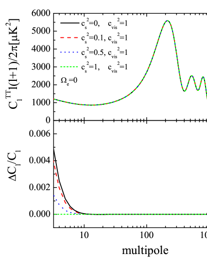
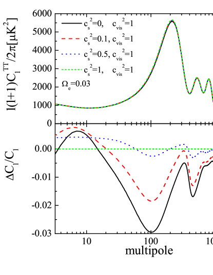
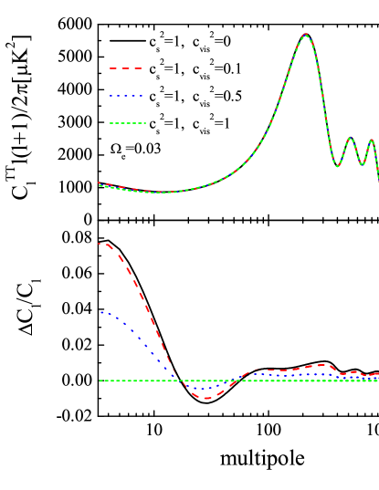
It is interesting to investigate if this competition between $c_{\rm s}^{2}$ and $c_{\rm vis}^{2}$ is still present in the case of a EDE scenario. For dark energy present at early epochs it may also contribute to the early Integrated Sachs Wolfe effect. In Figure 4 we plot the same spectra as in Figure 3 but now with an EDE contribution with $\Omega_{e}=0.03$. We see that now the spectra show a small difference around the first peak due to the different early integrated Sachs Wolfe effect. While the differences are small it is important to notice that at these scales the cosmic variance is significantly smaller than at large scales where the late-time ISW effect is important.

In addition to the (early and late) ISW effect, the presence of EDE also affects the evolution of the acoustic oscillations before recombination, leading to a signature at larger $l$’s than the ISW. If the sound speeds are increased, EDE perturbations get more suppressed, leading to a stronger decay of the metric perturbations. This in turn leads to a stronger boost of the amplitude of the acoustic oscillations. The (subtle) damping in the second peak is a sign that the potentials have not decayed as much as when perturbations are unimportant.

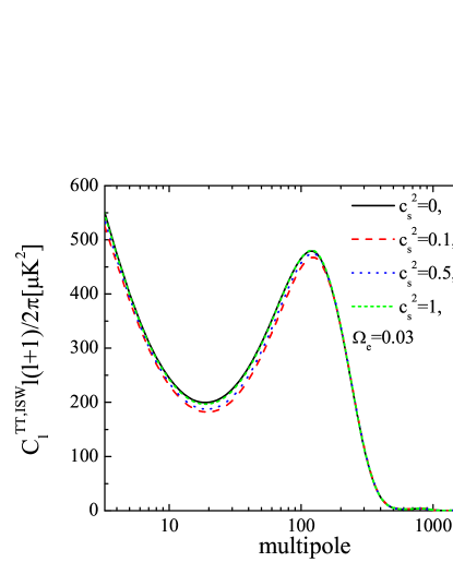
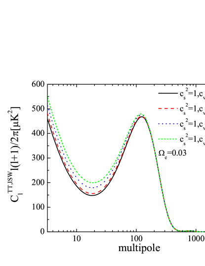
The ISW behaviour is better shown in Figure 5 where we plot just the ISW component of the temperature CMB anisotropy angular power spectrum. As we can clearly see, the behaviour of the ISW angular spectrum can be evidently divided into a contribution from the late ISW effect on large angular scales ($\ell<30$) and a contribution from the early ISW, producing a peak on degree scales at $\ell\sim 120$. While variations on large scales are negligible compared to cosmic variance errors, perturbations introduce signal via the early ISW term that is more significant. We can therefore expect that in the EDE scenario perturbations can play a more significant role than in a standard late dark energy scenario. The perturbations also influence gravitational lensing of the CMB, as we discuss in the next section.

Figure 5: As Figure 4, with an early dark energy density $\Omega_{\rm e}=0.03$, but now focusing on only the ISW component to show the effects of the sound speeds. The left rise is due to the late ISW effect while the bump is principally coming from early ISW.

III.2 CMB Lensing

Gravitational lensing of the CMB can improve significantly the CMB constraints on several cosmological parameters (see e.g. Perotto:2006rj ; calabrese ), since it is strongly connected with the growth of perturbations and gravitational potentials. The effect of weak lensing is to remap the direction of observation (see e.g. IE ; Lewis:2006fu ; Okamoto2003 ) from ${\bf n}$ to ${\bf n}^{\prime}={\bf n}+{\bf d}({\bf n})$ where ${\bf d}({\bf n})$ is the lensing deflection angle.

The lensing deflection angle power spectrum, or equivalently the convergence power spectrum, is related to the lensing potential spectrum $C_{l}^{\phi\phi}$, through :

$$C_{l}^{dd}=l(l+1)C_{l}^{\phi\phi}\ .$$ (6)

Figure 6: Lensing potential power spectra for different standard and early dark energy scenarios with $c_{\rm s}^{2}$ and $c_{\rm vis}^{2}$ varying from $0$ to $1$.

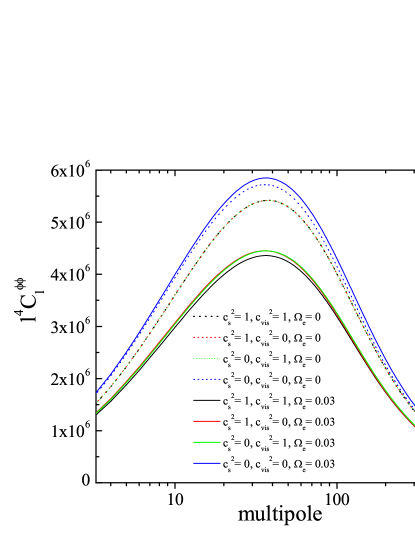
Figure 6 shows the lensing potential angular spectra for scenarios with and without EDE and for different values of $c_{\rm s}^{2}$ and $c_{\rm vis}^{2}$. The plot shows a nontrivial dependence of the lensing angular spectrum on $c_{\rm s}^{2}$, $c_{\rm vis}^{2}$, and $\Omega_{e}$, with some degeneracies clearly present. Basically, suppressing perturbations by taking $c_{\rm vis}^{2}=1$ or $c_{\rm s}^{2}=1$ (or both) are nearly equivalent. Only when perturbations are maximally allowed, through $c_{\rm vis}^{2}=0$ and $c_{\rm s}^{2}=0$ together, is the lensing power significantly enhanced. In this case, early dark energy plays a major role, yielding a 30% enhancement in power, while the model with no early dark energy only sees a $\sim 6\%$ boost relative to its no-perturbation case. We therefore expect the lensing signal to predominantly improve the constraints when combined with observations of the primary CMB signal. From Fig. 6 we expect largest improvements on early dark energy, but less so on $c_{\rm vis}^{2}$ and $c_{\rm s}^{2}$, except when they both take on low values. We verify this numerically in Sec. IV.

III.3 CMB Experiments and Forecasting

To evaluate the future constraints on EDE models we consider the Planck planck and CMBPol Bock:2009xw experiments using three frequency channels for each with the experimental specifications as listed in Table 1 below.

Experiment	Channel[GHz]	FWHM	$\sigma_{T}[\mu K]$	$\sigma_{P}[\mu K]$
Planck	143	7.1’	6.0	11.4
$f_{sky}=0.85$	100	10.0’	6.8	10.9
	70	14.0’	12.8	18.3
CMBPol	150	5.6’	0.177	0.250
$f_{sky}=0.85$	100	8.4’	0.151	0.214
	70	12.0’	0.148	0.209

Table 1: Planck and CMBPol experimental specifications.

We consider for each frequency channel a detector noise of $(\theta\sigma)^{2}$ where $\theta$ is the FWHM of the beam assuming a Gaussian profile and $\sigma$ is the sensitivity. We therefore add to each $C_{\ell}$ fiducial spectrum a noise spectrum given by :

$$N_{\ell}^{X}=(\theta\sigma_{X})^{2}\,e^{l(l+1)/l_{b}^{2}}\,,$$ (7)

where $l_{b}\equiv\sqrt{8\ln 2}/\theta$ and the label $X$ refers to either temperature or polarization, $X=T,P$.

When CMB lensing information is also included we add to our dataset the lensing deflection angle power spectrum (and the corresponding noise spectrum). At sufficiently large angular scales ($l\lesssim 1000$), contributions to the deflection field will come mainly from the linear regime and, in harmonic space, the power spectrum of the deflection field reads :

$$\langle a_{lm}^{d*}a_{l^{\prime}m^{\prime}}^{d}\rangle=\left(C_{l}^{dd}+N_{l}^{dd}\right)\delta_{ll^{\prime}}\delta_{mm^{\prime}},$$ (8)

where $a_{lm}^{d}$ can be considered as an approximately Gaussian variable Okamoto2003 . The noise power spectrum $N_{l}^{dd}$ reflects the errors in the deflection map reconstruction. We estimate the lensing contribution with the quadratic estimator method of Hu & Okamoto Okamoto2003 based on the correlations between five possible pairs of maps: $TT$, $EE$, $TE$, $TB$, $EB$ (since the $B$-mode signal is dominated by lensing on small scales, the estimator $BB$ cannot be used in this method). $N_{l}^{dd}$ corresponds to the minimal noise spectrum achievable by optimally combining the five quadratic estimators. Finally, the non-vanishing correlations between the temperature and the deflection maps are :

$$\langle a_{lm}^{T*}a_{l^{\prime}m^{\prime}}^{d}\rangle=C_{l}^{Td}\delta_{ll^{\prime}}\delta_{mm^{\prime}}~{}.$$ (9)

Following the description in Perotto:2006rj we generate $C_{l}^{dd}$, $C_{l}^{Td}$ and $N_{l}^{dd}$ power spectra and include these datasets in the analysis, both for Planck and CMBPol.

To get a general sense of the parameter constraints and degeneracies, we first perform a Fisher matrix analysis. The Fisher matrix is defined as :

$$F_{ij}\equiv\Bigl{\langle}-\frac{\partial^{2}\ln\mathcal{L}}{\partial p_{i}\partial p_{j}}\Bigr{\rangle}_{p_{0}}$$ (10)

where $\mathcal{L}({\rm data}|{\bf{p}})$ is the likelihood function of a set of parameters ${\bf p}$ given some data; the partial derivatives and the averaging are evaluated using the fiducial values ${\bf p_{0}}$ of the parameters. The Cramér-Rao inequality implies that $(F^{-1})_{ii}$ is the smallest variance in the parameter $p_{i}$, so we can generally think of $F^{-1}$ as the best possible covariance matrix for estimates of the vector ${\bf p}$. The one sigma error for each parameter is then defined as :

$$\sigma_{p_{i}}=\sqrt{(F^{-1})_{ii}}.$$ (11)

The Fisher matrix for a CMB experiment is given by (see fishcmb ) :

$$F^{\rm CMB}_{ij}=\sum_{l=2}^{l_{\rm max}}\sum_{\alpha,\beta}\frac{\partial C_{l}^{\alpha}}{\partial p_{i}}({\rm Cov}_{l})_{\alpha\beta}^{-1}\frac{\partial C_{l}^{\beta}}{\partial p_{i}},$$ (12)

where $\alpha$ and $\beta$ are running indexes over the angular power spectra $C_{l}$. For example we include temperature TT, temperature-polarization TE, E mode polarization EE, or TT, Td, dd in the case with CMB lensing. ${\rm Cov}_{l}$ is the spectra covariance matrix. We use information in the power spectra out to $l_{\rm max}=3000$.

IV Results

IV.1 Constraints from Planck and CMBPol

We consider a set of $9$ cosmological parameters with the following fiducial values: the physical baryonic and cold dark matter densities relative to critical $\Omega_{b}h^{2}=0.02258$ and $\Omega_{c}h^{2}=0.1109$, the optical depth to reionization $\tau=0.088$, the Hubble parameter $H_{0}=71\,{\rm km/s/Mpc}$, the current dark energy equation of state $w_{0}=-0.90$, the early dark energy density relative to critical $\Omega_{\rm e}=0.03$, the spectral index $n_{s}=0.963$, and finally the effective and viscous sound speeds $c_{\rm s}^{2}$ and $c_{\rm vis}^{2}$. In order to check the stability of the result under the assumption of the fiducial values for $c_{\rm s}^{2}$ and $c_{\rm vis}^{2}$ we investigate several different pairs of values. CMB lensing is always included except for the comparison in Table 2.

Using the method described above we forecast the constraints on $w_{0}$ and $\Omega_{e}$. We find that both Planck and CMBPol can constrain with high accuracy those parameters. Planck will obtain $\sigma_{w_{0}}^{\rm Planck}=0.10$ while CMBPol can improve this by an order of magnitude to $\sigma_{w_{0}}^{\rm CMBPol}=0.01$. The density in EDE will also be well constrained by Planck, with $\sigma_{\Omega_{e}}^{Planck}=0.004$, while CMBPol can improve by a factor four to $\sigma_{\Omega_{e}}^{\rm CMBPol}=0.001$ (see also Table 3). We find no significant dependence of these constraints on the choice of the fiducial values of the EDE perturbation parameters $c_{\rm s}^{2}$ and $c_{\rm vis}^{2}$. Figure 7 shows the 2-dimensional likelihood plots in the $w_{0}$-$\Omega_{\rm e}$ plane for both Planck and CMBPol experimental configurations. These results are for the case $c_{\rm vis}^{2}=c_{\rm s}^{2}=0.33$, but again, there is no practically change in the contours for different choices of $c_{\rm s}^{2}$ or $c_{\rm vis}^{2}$.

Figure 7: 68% and 95% c.l. likelihood contours for Planck (solid line) and CMBPol (dashed line). The ‘+’ symbol represents the fiducial values.

The expected $1$-$\sigma$ constraints on EDE perturbation parameters $c_{\rm s}^{2}$ and $c_{\rm vis}^{2}$ are presented in Table 2 for Planck and for CMBPol experiments. We show the constraints obtained both with and without CMB lensing data.

		No lensing				With lensing
Fiducial	Fiducial	Planck	CMBPol	Planck	CMBPol	Planck	CMBPol	Planck	CMBPol
$c_{\rm vis}^{2}$	$c_{\rm s}^{2}$	$\sigma_{c_{\rm vis}^{2}}$	$\sigma_{c_{\rm vis}^{2}}$	$\sigma_{c_{\rm s}^{2}}$	$\sigma_{c_{\rm s}^{2}}$	$\sigma_{c_{\rm vis}^{2}}$	$\sigma_{c_{\rm vis}^{2}}$	$\sigma_{c_{\rm s}^{2}}$	$\sigma_{c_{\rm s}^{2}}$
0.01	0.1	0.019	0.008	0.027	0.013	0.016	0.007	0.023	0.010
0.1	0.1	0.075	0.037	0.093	0.043	0.067	0.038	0.082	0.031
0.33	0.1	0.17	0.081	0.11	0.064	0.16	0.092	0.10	0.051
1	0.1	0.52	0.27	0.12	0.074	0.42	0.20	0.11	0.057
0.33	0.33	0.24	0.14	0.16	0.11	0.21	0.12	0.15	0.10
0.1	0.01	0.094	0.048	0.029	0.014	0.084	0.032	0.022	0.012
0.1	0.1	0.075	0.037	0.093	0.043	0.067	0.038	0.082	0.031
0.1	0.33	0.098	0.061	0.10	0.074	0.092	0.058	0.11	0.072
0.1	1	0.19	0.10	0.71	0.35	0.17	0.091	0.68	0.33

Table 2: Fisher analysis results at 68% c.l. for several different values of $c_{\rm s}^{2}$ and $c_{\rm vis}^{2}$, for Planck and for CMBPol datasets, with and without CMB lensing included in the analysis.

Figure 8: 68% and 95% c.l. likelihood contours for Planck (solid line) and CMBPol (dashed line). In the upper panel the fiducial values are $c_{\rm vis}^{2}=0.1$ and $c_{\rm s}^{2}=1$, in the middle one $c_{\rm vis}^{2}=1$ and $c_{\rm s}^{2}=0.1$, in the lower panel an intermediate case with $c_{\rm vis}^{2}=c_{\rm s}^{2}=0.33$ is reported. The ‘+’ symbol represents the fiducial values. Note the different scales.

From the results listed in Table 2 we can derive the following conclusions about estimating $c_{\rm vis}^{2}$ and $c_{\rm s}^{2}$:

• Including CMB lensing improves the constraints by $\sim 10-20\%$ (as compared to $50-60\%$ for $\Omega_{e}$ and $5-10\%$ for $w_{0}$).

• CMBPol provides constraints that are generally a factor $\sim 2$ better than Planck.

• The constraints on $c_{\rm s}^{2}$ (or $c_{\rm vis}^{2}$) depend strongly on the assumed value of $c_{\rm vis}^{2}$ (respectively $c_{\rm s}^{2}$), the general trend being that the uncertainties grow with the fiducial values. For example, assuming $c_{\rm s}^{2}=0.1$, the $1$-$\sigma$ error on this parameter will increase by a factor $\sim 5$ if the fiducial model moves from $c_{\rm vis}^{2}=0.01$ to $c_{\rm vis}^{2}=1$. At the same time, assuming $c_{\rm vis}^{2}=0.1$, the $1$-$\sigma$ error on this parameter will increase by a factor $\sim 2$ if the fiducial model moves from $c_{\rm s}^{2}=0.01$ to $c_{\rm s}^{2}=1$.

• The strong correlation between $c_{\rm s}^{2}$ and $c_{\rm vis}^{2}$ makes it difficult to precisely measure these parameters individually with either Planck or CMBPol (and of course the situation worsens as $\Omega_{\rm e}$ decreases or $w_{0}$ approaches $-1$).

The correlation between EDE perturbation parameters can be clearly seen in Figure 8, where we plot the $68\%$ and $95\%$ c.l. 2-D likelihood contour plots in the $c_{\rm s}^{2}$-$c_{\rm vis}^{2}$ plane. The solid lines are the constraints derived from Planck while the dashed lines are from CMBPol. A reasonable way of quantifying how well the sound speed and viscosity sound speed can be constrained is by asking at what significance level a non-standard value of $c^{2}_{s}$ or $c^{2}_{vis}$ can be distinguished from the standard (quintessence) value, i.e. from $c^{2}_{s}=1$ or $c^{2}_{vis}=0$. By this metric, whether or not the Planck and CMBpol experiments provide much insight of course depends on the fiducial values of $c^{2}_{s}$ and $c^{2}_{vis}$. For example, for the $c^{2}_{s}=0.1$ and $c^{2}_{vis}=1$ fiducial model (middle panel), Planck could rule out a perfect fluid (i.e. $c^{2}_{vis}=0$) at about $2\sigma$ and CMBpol could do this at more than $4\sigma$. However, for the $c^{2}_{s}=1$ and $c^{2}_{vis}=0.1$ fiducial model (top panel), neither experiment can rule out a perfect fluid. Similarly, for the fiducial in the middle panel, both experiments can rule out $c_{s}^{2}=1$ (quintessence) at very high significance, but not for a fiducial value of $c_{s}^{2}$ significantly closer to unity.

The fact that the uncertainties and ellipse shapes depend strongly on the fiducial parameter values means that the Fisher matrix evaluated at the fiducial model is not a good predictor of the shape of the likelihood function away from the fiducial model (and that the likelihood function is thus far from Gaussian). Hence, away from the fiducial, the true constant likelihood contours could be quite different from the ones calculated using the Fisher matrix. This means one has to be cautious when making estimates as in the previous paragraph. For example, from the middle panel of Figure 8, we estimated that Planck would rule out $c^{2}_{vis}=0$ at about $2\sigma$, i.e. at $95\%$ confidence level. However, since the uncertainty in $c^{2}_{vis}$ decreases strongly as the fiducial value is lowered, the true significance may in this case be higher than $95\%$. However, this subtlety does not affect the main point made in the previous paragraph, namely that for a range of reasonable values of $c_{s}^{2}$ ($c^{2}_{vis}$), both Planck and CMBpol will be able to rule out the canonical value, although CMBpol with much more significance. In section IV.5, we check our Fisher results using an MCMC analysis of the true non-Gaussian likelihood and we find that our Fisher estimates of uncertainties and error ellipses calculated are quite accurate.

IV.2 Including Supernovae

Since the early dark energy component changes the Hubble parameter and luminosity distances, Type Ia supernovae (SN) information can be very useful to break geometrical degeneracies.

Each SN magnitude measurement can be expressed as:

$$m_{i}=5\log_{10}[H_{0}d_{L}(z_{i},w_{0},\Omega_{m},\Omega_{\rm e})]+{\mathcal{M}}+\epsilon_{i}$$ (13)

where $d_{L}$ is the luminosity distance, ${\mathcal{M}}$ is a combination of the SN absolute magnitude and Hubble constant, and $\epsilon$ is a zero mean random term including all systematic and measurement errors. Given $N$ SN at redshifts $z_{1}$…$z_{N}$, we can describe the measured data $m_{i}$ as an N-dimensional vector m. Assuming Gaussian errors $\epsilon_{i}$, the Fisher matrix is given by (see tegmark ) :

$$F^{\rm SN}_{ij}=\frac{1}{2}{\rm Tr}[C^{-1}\frac{\partial C}{\partial p_{i}}C^{-1}\frac{\partial C}{\partial p_{j}}]+\frac{\partial{\bm{\mu}}^{T}}{\partial p_{i}}C^{-1}\frac{\partial{\bm{\mu}}}{\partial p_{j}},$$ (14)

where ${\bm{\mu}}\equiv\langle{\bm{m}}\rangle$ is the vector of mean magnitudes and $C\equiv\langle{\bm{m}}{\bm{m}}^{T}\rangle-{\bm{\mu}}{\bm{\mu}}^{T}$ is the covariance matrix of magnitudes. The parameter vector ${\bm{p}}$ for the SN Fisher matrix includes $\Omega_{m}$, $\Omega_{\rm e}$, $w_{0}$, and the nuisance parameter ${\mathcal{M}}$.

For future SN data we consider 1800 SN out to $z=1.5$ (roughly with a cut SNAP distribution klmm ) plus 300 local ($z=0.05$) SN, with an intrinsic dispersion of 0.1 mag and a systematic error of $0.02(1+z)/2.7$ per $0.1$ bin in $z$ added in quadrature. New EDE parameters errors, reported in Table 3, are estimated considering a total Fisher matrix :

$$F^{\rm TOT}_{ij}=F^{\rm CMB}_{ij}+F^{\rm SN}_{ij}\ .$$ (15)

Parameter	Planck			CMBPol
uncertainty	alone		+SN	alone		+SN
$\sigma_{w_{0}}$	0.10		0.02	0.010		0.005
$\sigma_{\Omega_{\rm e}}$	0.004		0.003	0.001		0.001
$\sigma_{c_{\rm s}^{2}}$	0.15		0.15	0.10		0.09
$\sigma_{c_{\rm vis}^{2}}$	0.21		0.20	0.12		0.11

Table 3: 68% c.l. uncertainties on EDE parameters from Planck or CMBPol with and without SN distance information. The fiducial values $c_{\rm s}^{2}=c_{\rm vis}^{2}=0.33$ are used.

We see that the main improvement of adding SNe is on $w_{0}$, reducing the Planck uncertainty by a factor of 5, and the CMBPol one by a factor of 2. The SN measurements do not reach to high enough redshift to have a good handle on $\Omega_{\rm e}$ (the distance out to $z=2$ in a model with no early dark energy but $w_{a}=-(1/2)dw/d\ln a|_{z=1}=5\Omega_{\rm e}$ agrees nearly exactly with an EDE model linderbao , and $w_{a}$ cannot be determined so precisely). We also see that the perturbation parameters appear to be mostly uncorrelated with any parameters to which SN distances are sensitive (indeed, they will be correlated mostly with each other). It is not clear what probes are best for further constraining $c_{\rm s}^{2}$ and $c_{\rm vis}^{2}$, since CMB lensing (especially at the level of CMBPol) already includes matter power spectrum information. Perhaps three-dimensional weak lensing and galaxy statistics, or nonlinear structure, would supply more leverage. We leave this for future work.

IV.3 Including Massive Neutrinos

In addition to considering situations where the perturbation parameter constraints improve, we should also explore other parameters that might be degenerate with them, and so both weaken the constraints and be affected themselves by the presence of cold or stressed dark energy.

In particular it is interesting to study whether EDE could have any implication for the bounds on the neutrino mass from CMB experiments. Planck and CMBPol are indeed expected to provide new and very stringent bounds on the sum of neutrino masses $\sum m_{\nu}$, extremely competitive with respect to bounds coming from laboratory experiments as KATRIN Drexlin:2005zt .

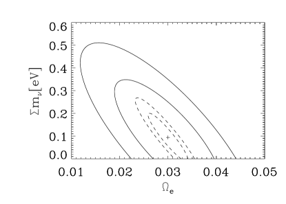
We performed a new Fisher matrix analysis adding to our 9-dimensional set of cosmological parameters the neutrino energy density, $\Omega_{\nu}h^{2}$, with a fiducial value of $0.001$ (corresponding to $\sum m_{\nu}\approx 0.09$ eV; we quote all results in terms of $\sum m_{\nu}=94\Omega_{\nu}h^{2}\,{\rm eV}$). In Figure 9 we report the constraints from Planck and CMBPol and as we can see there is an anticorrelation between $\Omega_{e}$ and $\sum m_{\nu}$ for both Planck and CMBPol experiments. This means that future CMB bounds on the neutrino mass can be affected by the presence of an EDE component (also see dep0901 ) . Numerical results are reported in Table 4. In particular, we studied the impact of one component on the other. As we can see from the Table the presence of early dark energy and massive neutrinos almost doubles the uncertainty on both of these parameters.

Model	Planck		CMBPol
	$\sigma_{\Omega_{\rm e}}$	$\sigma_{\sum m_{\nu}}$	$\sigma_{\Omega_{\rm e}}$	$\sigma_{\sum m_{\nu}}$
$\Omega_{\rm e}=0$	–	0.09	–	0.02
$\sum m_{\nu}=0$	0.004	–	0.001	–
$\Omega_{\rm e},\sum m_{\nu}\neq 0$	0.007	0.20	0.003	0.07

Table 4: 68% c.l. uncertainties on EDE density and neutrino density from Planck and CMBPol, including marginalization over the perturbation parameters $c_{\rm s}^{2}$ and $c_{\rm vis}^{2}$.

Figure 9: 68% and 95% c.l. likelihood contours for Planck (solid line) and CMBPol (dashed line). The degeneracy between $\Omega_{e}$ and $\sum m_{\nu}$ means that the constraint on $\sum m_{\nu}$ is affected by the inclusion of an EDE component, by a factor 2–3 as seen in Table 4.

Moreover a wrong assumption of the $\Omega_{\rm e}$ fiducial value (e.g. ignoring early dark energy) can bias the estimation of other parameters and in particular of neutrino mass, as we now discuss.

IV.4 Bias from Neglecting Perturbations

With the Fisher matrix formalism we can also evaluate the bias generated in parameter estimation when analyzing the datasets assuming a wrong fiducial model, e.g. fixing $c_{\rm vis}^{2}$ to the wrong value.

For a Gaussian likelihood function, the bias in the $i$-th cosmological parameter, $\delta\theta_{i}$, caused by the discrepancy between the assumed value of a parameter $\psi_{j}$ and its true value, $\delta\psi_{j}$, is given by Knox_Scocc_Dod ; Huterer_Turner ; DeBernardis:2008tk :

$$\delta\theta_{i}=-[F^{\theta\theta}]^{-1}_{ki}F^{\theta\psi}_{kj}\delta\psi_{j}$$ (16)

where $F^{\theta\theta}$ is the Fisher matrix in the space of $\theta_{i}$ parameters, and $F^{\theta\psi}$ is a Fisher submatrix with derivatives with respect to the assumed bias parameters $\psi_{j}$ and the measured parameters $\theta_{i}$.

In our case we want to study the effect of fixing $c_{\rm vis}^{2}=0$ when an input (“true”) model has $c_{\rm vis}^{2}=0.33$. Figure 10 shows the shift obtained on the early dark energy parameters $c_{\rm s}^{2}$, $w_{0}$, and $\Omega_{\rm e}$. We plot 2-dimensional contours showing the degeneracies at $68\%$ and $95\%$ confidence levels for Planck in the left panels and CMBPol in the right panels. The solid lines are the results obtained including $c_{\rm vis}^{2}$ in the parameter marginalization, while the dashed lines are the contours obtained when $c_{\rm vis}^{2}$ is (incorrectly) fixed to $0$.

(a)	(b)

Figure 10: 68% and 95% c.l. contour plots in the $\Omega_{\rm e}$-$c_{\rm s}^{2}$ (top panels) and $\Omega_{e}$-$w_{0}$ (bottom panels) planes for Planck (panel (a)) and CMBPol (panel (b)). The fiducial model has always $c_{\rm vis}^{2}=0.33$. The solid lines are the results obtained correctly including $c_{\rm vis}^{2}$ in the parameter estimation, while the dashed lines are the biased contours obtained when $c_{\rm vis}^{2}$ is assumed to be 0 (i.e. ignoring viscosity). The ‘+’ symbol represents the original fiducial values, while the ‘$\ast$’ symbol gives the shifted values.

As expected the constraint on $c_{\rm s}^{2}$ can be affected by a wrong assumption on $c_{\rm vis}^{2}$. Assuming a value of $c_{\rm vis}^{2}$ lower than the truth is like assuming more perturbations, so $c_{\rm s}^{2}$ must be biased high to compensate and reduce the perturbations. The resulting best fit value is $\sim 1$-$\sigma$ away from the fiducial value for Planck, and $\sim 2$-$\sigma$ away for CMBPol. The other parameters are only mildly biased.

When massive neutrinos are considered, $\Omega_{\rm e}$ will play the major role and will strongly affect $\sum m_{\nu}$. In particular we study the effect of neglecting early dark energy (i.e. fixing $\Omega_{\rm e}=0$) when an input true model with $\Omega_{\rm e}=0.03$ is used. This assumption will shift $\sum m_{\nu}$ from its true value of $0.09\,{\rm eV}$ to $0.59\,{\rm eV}$ and $0.65\,{\rm eV}$ for Planck and CMBPol respectively – excluding the true value by $28\sigma$ in the latter case!

IV.5 Comparisons with MCMC

Because the Fisher matrix forecasts are sometimes biased, especially in case where there is a strong degeneracy between parameters, we check our previous results with the analysis that maps out the full likelihood function in the cosmological parameters. The analysis uses the publicly available MCMC package cosmomc Lewis:2002ah with a convergence diagnostic done through the Gelman and Rubin statistic. We sample the following 11-dimensional set of cosmological parameters, adopting flat priors on them: the baryon and cold dark matter densities $\omega_{\rm b}$ and $\omega_{\rm c}$, the Hubble constant $H_{0}$, the scalar spectral index $n_{S}$, the overall normalization of the spectrum $A$ at $k=0.05$ Mpc^-1, the optical depth to reionization, $\tau$, the current equation of state parameter $w_{0}$, the early dark energy density $\Omega_{\rm e}$, the dark energy sound speed $\log c_{\rm s}^{2}$, the viscosity sound speed $c_{\rm vis}^{2}$, and the neutrino masses $\sum m_{\nu}$. We consider purely adiabatic initial conditions and we impose spatial flatness. We moreover only consider $w_{0}$ values greater than $-1$. The fiducial model for generating the mock data uses the WMAP seven year best fit cosmological parameters values, plus $w_{0}=-0.9$, $\Omega_{\rm e}=0.03$, $c_{\rm vis}^{2}=0.33$ and $c_{\rm s}^{2}=1$.

The results obtained are in good agreement with Fisher constraints, recovering the fiducial value at the $1\sigma$ level for all the parameters. Moreover, the MCMC errors are in good agreement with the Fisher matrix error estimates, as reported in Table 5.

Parameter	Fisher	MCMC
$w_{0}$	0.10	0.10
$\Omega_{\rm e}$	0.004	0.007
$c_{\rm s}^{2}$	0.73	0.74
$c_{\rm vis}^{2}$	0.26	0.27

Table 5: 1-$\sigma$ errors from Fisher matrix and MCMC analysis on EDE parameters from Planck dataset.

V Discussion

In this paper we have investigated future constraints on EDE models achievable by Planck and CMBPol experiments. We included CMB lensing as a probe, and the possibilities of a sound speed less than the speed of light and of anisotropic stresses in the clustering of the dark energy component parameterized with a viscosity parameter $c_{\rm vis}^{2}$. Overall, the model can be viewed as “early, cold, or stressed dark energy”.

We have found that $c_{\rm vis}^{2}$ can be strongly correlated with the sound speed parameter $c_{\rm s}^{2}$. For this reason it will be difficult for these future experiments to derive significant constraints on these sound speed parameters individually, although finding a deviation from the standard quintessence with $c_{\rm s}^{2}=1$, $c_{\rm vis}^{2}=0$ will be possible.

We have also shown that neglecting the possibility of anisotropic stresses in EDE could significantly bias the constraints on EDE parameters.

The results, obtained through a Fisher Matrix formalism, have been checked by a Monte Carlo Markov Chain analysis on Planck synthetic data. We have considered SN information to break geometrical degeneracies and we have found this significantly improves the equation of state parameter estimation. Finally we have investigated the impact of EDE on the determination of the neutrino mass from CMB experiments and we found it to be significant. In particular, neglect or misestimation of early dark energy density can severely bias neutrino mass constraints for both Planck and CMBPol. Investigation of early, cold, or stressed dark energy is important not only to uncover further windows on the nature of dark energy and high energy physics, but to ensure that conclusions on other cosmological parameters are robust.