Selective Image Super-Resolution

Abstract

In this paper we propose a vision system that performs image Super Resolution (SR) with selectivity. Conventional SR techniques, either by multi-image fusion or example-based construction, have failed to capitalize on the intrinsic structural and semantic context in the image, and performed “blind” resolution recovery to the entire image area. By comparison, we advocate example-based selective SR whereby selectivity is exemplified in three aspects: region selectivity (SR only at object regions), source selectivity (object SR with trained object dictionaries), and refinement selectivity (object boundaries refinement using matting). The proposed system takes over-segmented low-resolution images as inputs, assimilates recent learning techniques of sparse coding (SC) and grouped multi-task lasso (GMTL), and leads eventually to a framework for joint figure-ground separation and interest object SR. The efficiency of our framework is manifested in our experiments with subsets of the VOC2009 and MSRC datasets. We also demonstrate several interesting vision applications that can build on our system.

1 Introduction

Super-resolution image reconstruction is the process to recover a high-resolution image from a single or multiple low-resolution input images [1]. In frequency domain, this corresponds to resolving the beyond-Nyquist high-frequency components from the aliased version of the spectrum  [2]. Apparently SR problem is under-determined by its nature, because practically many high-resolution images can produce the same low resolution image(s). Therefore it comes without surprise that the extensive research on SR has worked on providing additional constraints and/or incorporating various prior knowledge.

Figure 1: Visual applications of our selective SR system. (From left to right) zoom blurring, object pop-up, and image composition. (For better view, please refer to the electronic version)

Accordingly existing SR techniques can be broadly classified into two categories: 1) the classical multi-image fusion, and 2) the sophisticated example-based construction.

Multi-image fusion techniques normally require multiple images of the same scene with subpixel relative displacements as inputs. When sufficiently many such images are provided, direct SR reconstructions are feasible in both spatial and frequency domains via solving systems of linear equations. Even insufficient, these input images can be incorporated into explicit regularization frameworks with various kind of prior knowledge (mostly smoothness). A good review of all these techniques is provided in [1].

Figure 2: Overview of our selective image SR system. Given a low-resolution input image, our system first performs over-segmentation, and then employs GMTL (based on pre-trained dictionaries) to decide whether each segment belongs to the object region, leading to figure-ground separation. Image matting is used to refine the separation. It finally constructs super-solved version of the object region with the object dictionaries, and other special effects (zoom blur, part emboss) can be implemented by processing either the foreground or background region.

This family of SR algorithms are attractive due to the simplicity of algorithmic implementation, and the ease of multi-camera imaging and video capturing as inputs. As demonstrated by many authors [3, 4], however, fusion-based SR can only provide numerically less than double magnification factor. This has severely limited their use for many applications.

This limitation has been broken since the introduction of example-base SR techniques (or Image Hallucination) [3, 5]. Techniques in this vein feature learning low- and high-resolution image patches from a collection of low- and high-resolution image pairs. Upon completion of the learning phase, early developed algorithms (e.g. [3, 5, 6, 7]) involve finding matched high-resolution patch for each low-resolution input and simply taking the high-resolution as the recovered. These selection-based methods normally entail large training datasets to ensure the desired high-resolution patches can be best approximated by existing training patches. By comparison, recent developments (c.f. [8, 9, 10]) have introduced additional flexibility and scalability by treating the patch generation process as regression problems over properly trained/selected basis patches. This innovation has made SR accessible to a wide range of applications with training sets of manageable sizes.

Despite the credible success SR research has made over the decades, it is misfortune of SR being treated isolated as a simple image enhancement process. In view of the integral nature of vision research, it is reasonable that one starts to link SR with other computer vision tasks, such as figure/ground separation, weak object identification. In fact, it has been realized before that “blind” SR reconstruction to the whole image area may not work well, in terms of e.g. resulting in over-smooth edges and corners [11]. To mitigate the adverse effect, SR algorithms may be made adaptive to specific image regions. In other words, the intrinsic image structure (such as edges, region segments) and even the semantic context of image regions (such as spatial layout, figure/ground separation, localized labels for regions) need to be explicitly accounted for. This coincides with the ongoing theme of recognition-oriented vision research, namely building the synergy between shape and appearance modeling (e.g. epitomic shape and appearance modeling [12] and region-based recognition [13]). Furthermore, the coincidence sheds light on integration of SR reconstruction with other typical vision tasks, such as segmentation, recognition.

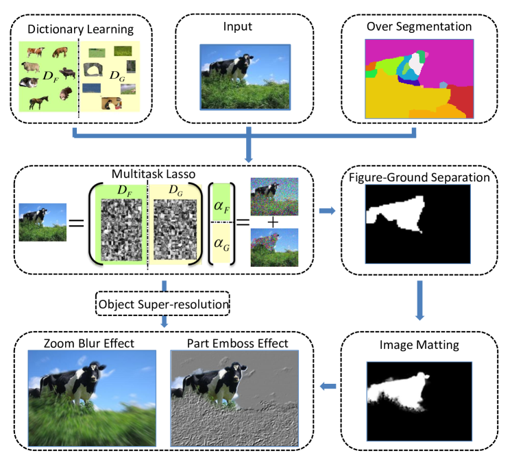
Moving towards this direction, we propose an image SR system with selectivity. Compared to conventional SR algorithms, selectivity is exercised in three modules of the system: 1) perform SR only at object region(s) and blur out the background region (region selectivity), 2) generate super-resolved patches from training dictionaries of objects rather than background (dictionary selectivity), and 3) refine the figure/ground boundaries with alpha matting techniques [14, 15] (refinement selectivity). Three levels of selectivity has been facilitated by neat integration/adaptation of several state-of-the-art techniques, including image over-segmentation, sparse coding dictionary learning, multitask lasso, and image matting. Overall, the proposed system is able to separate the foreground objects out of the image region, perform SR to the object region and yield visually pleasing results after matting and other simple post-processings. Figure 1 provides three special visual effects for a single input low-resolution image. Figure 2 gives an overview of our system pipeline and various techniques involved.

2 Related Work

The current work follows the line of example-based SR, which dates back to the seminal papers [5, 4]. In these pioneering works, techniques such as Markov random field (MRF) with belief propagation (BP) and hierarchical nearest neighbor matching were used to establish the low- to high-resolution patch correspondences. Thereafter, [11] introduced the primal sketch priors to improve the reconstruction at the blurred edges, ridges, and corners. All these early example-based SR techniques assume that the recovered patches are to be selected from the training datasets. This inevitably requires a large-scale datasets for satisfactory patch approximation and hence reconstruction. This limitation of the selection paradigm triggers the development of the regression paradigm, in which novel patches can be generated from a (usually linear) combination of the existing. In this aspect, [8] and [10] used respectively a linear combination of several nearest neighboring patches and a sparsest combination of training patches to approximate the input low-resolution patch, and hence the low- and high-resolution correspondences. Our work is inspired by [10] which applied sparsity priors to SR.

Sparse coding traces its root in signal processing and compression, and is very recently introduced to the vision community for face recognition [16] and many other vision tasks [17]. Recent research in learning techniques has extended sparse coding to multiple-task or multi-label decision scenarios [18, 19, 20], whereby sparsity is exploited for feature selection and semantic inference. Another direction of extension is on unsupervised or weakly supervised structure discovery or over-complete coding dictionary learning [21, 22, 23]. These formulations explicitly require learned visual structures or patterns (encoded as visual dictionary parallel with the popular “bag-of-features” technique) facilitate sparse reconstruction. The current work builds on both extensions and tunes them to our selective SR applications.

The theme of joint vision problem solving exhibited by the current work is not novel. In recognition-oriented vision research, possibilities and advantages of joint visual object segmentation, detection, and recognition and analysis have been suggested in many works, e.g. the most recent ones [13, 24]. Our proposal of simultaneous object/background (or simply figure/ground) separation and SR reconstruction moves along the same line, hoping to discover new possibilities. Our empirical results seem to provide us with positive answers.

Alpha matting is used for accurate extraction of image foreground with transparent boundaries [14, 15]. One of the great challenges in matting is to obtain an initial figure-ground separation map (the “trimap”) of decent accuracy. The output from figure-ground separation of our algorithm (from the solution to the GMTL as explained later) has fractional accuracy and can be used for this purpose. Matting is used to fine-tune the boundary regions of our highlighted foreground object.

3 Image SR with Selectivity

Our selective SR system stems from the confluence of computer vision, machine learning and graphics techniques. Amongst them, the hardcore mid-level vision research in image segmentation, developments and applications of sparse coding and its derivatives such as the multi-task Lasso and (sparsity-induced) dictionary learning, and the extensively researched alpha matting process, are integrated into our system. This part will overview these techniques and provide some necessary details, following the pipeline of our framework (as in Figure 2).

3.1 Image Segmentation

Image segmentation has been one of the central topics in mid-level computer vision, accounting for “visual grouping” advocated by the Gestalt school of visual perception. Literally, image segmentation is the partitioning of an image into coherence groups of pixels, such that each group corresponds to semantic-level objects or parts of objects. The criterion for grouping is normally based on multiple image cues, such as pixel intensity, color, texture, motion as bottom-up driving force and categorical prior knowledge for top-down modulation.

Albeit the extensive research on image segmentation ever since the early vision days and the general belief that recognition and alike high-level vision tasks should be founded on segmentation, incorporating segmentation with other high-level vision tasks has not seen much success. This is in part because of the lack in a reliable and efficient segmentation algorithm up to date, and fundamentally determined by the fact that visual segmentation is inherently hierarchical and task-driven. Whereas object-level segmentation in general relies also on the top-down semantic-level knowledge, part-level segmentation tends to be much easier as it is mainly driven by bottom-up low-level features. Hence the latter is much better researched and normally leads to “over-segmentation”.

For our application, over-segmented image regions as the unit blocks for figure-ground analysis carries over the structural and patch contextual information. We assume homogeneity within each segmented region and the general consistency in choosing source patches for SR reconstruction. For implementation, we use the graph-based image segmentation of [25]. This algorithm uses very simple and intuitive measure for the local evidence of boundaries, and makes greedy decisions of segmentation that respect global structures and properties. Moreover, this algorithm has approximately linear complexity $\mathcal{O}\left(n\log n\right)$ w.r.t. the number of edges, where $n$ is the number of image pixels (the graph is not fully connected).

3.2 Sparse Coding and Dictionary Learning

The input low-resolution image and its over-segments obtained above will work with dictionaries trained this part towards figure-ground separation via GMTL. The dictionary training is closely related to the sparse coding technique. In signal processing, sparse coding refers to the problem of encoding signals (vector $\mathbf{y}$) as sparse (few nonzero coefficients) as possible, over known or unknown basis (matrix $\mathbf{D}\in\mathbb{R}^{p\times n}$, every column a $p$-dimensional basis vector). The basis is usually overcomplete, meaning $n\gg p$. If $\mathbf{D}$ is known, the problem is normally formulated as locating the sparest coefficient vector $\bm{\alpha}^{*}$ from the combinatorial optimization

$$\min_{\bm{\alpha}}\|\bm{\alpha}\|_{0},\;\text{s.t.}\;\mathbf{y}=\mathbf{D}\bm{\alpha}.$$ (1)

The optimization is NP-hard, and in practice for $\bm{\alpha}$ with notable sparsity, it can be relaxed as a $\ell_{1}$ convex optimization problem [26]

$$\min_{\bm{\alpha}}\|\bm{\alpha}\|_{1},\;\text{s.t.}\;\mathbf{y}=\mathbf{D}\bm{\alpha}.$$ (2)

To account for practical noisy cases, the equality constraint is normally relaxed as $\|\mathbf{y}-\mathbf{D}\widetilde{\bm{\alpha}}\|_{2}^{2}\leq\epsilon$, or in its Lagrangian form as

$$\min_{\widetilde{\bm{\alpha}}}\|\widetilde{\bm{\alpha}}\|_{1}+\lambda\|\mathbf{y}-\mathbf{D}\widetilde{\bm{\alpha}}\|_{2}^{2},$$ (3)

which is commonly known to the statistical learning community as Lasso and can be solved efficiently using the popular Least Angle Regression (LAR, [27]) method or the stochastic cyclic coordinate descent method [28]. Recently there is growing interest in the cases of sparse coding without known basis. Intuitively, learning the basis from the data can create more specialized basis system, and also reveals the underlying structure and helps discover prototypical samples from the data source alone (example applications in [21]). This is termed as “(sparsity-induced) dictionary learning”. Formally, to extract a dictionary $\mathbf{D}\in\mathbb{R}^{p\times n}$ of size $n$ from $m$ data samples $\left\{\mathbf{y}_{i}\right\}_{i=1}^{m},\mathbf{y}_{i}\in\mathbb{R}^{p}$ ($n<m$), the following optimization problem is to tackle

$$\min_{\left\{\widetilde{\bm{\alpha}}_{i}\right\}_{i=1}^{m},\mathbf{D}}\;\;\sum_{i=1}^{m}\left(\|\widetilde{\bm{\alpha}}_{i}\|_{1}+\lambda\|\mathbf{y}_{i}-\mathbf{D}\widetilde{\bm{\alpha}}_{i}\|_{2}^{2}\right).$$ (4)

The objective is convex with respect to each group of the variables, but not simultaneously. Hence one possible solution scheme is to alternate between the dictionary learning, i.e. solving for $\mathbf{D}$ given $\left\{\tilde{\bm{\alpha}}_{i}\right\}_{i=1}^{m}$, and the converse in the consequent step. This is exactly the strategy suggested in [21]. In our application, we find the online dictionary learning algorithm proposed in [22] much more efficient. This online solution is based on sequential solutions to quadratic local approximation of the objective function and has proven convergence. Our dictionary learning involves object images of $5$ known semantic classes and their pixel-level segmentation (detailed in experiment part). Image patches (typically of size $3\times 3$ or $5\times 5$ pixels) are randomly sampled from both object regions and their corresponding backgrounds. Sampled patches are used for training a pair of sparsity-induced dictionaries of a particular object class and the related backgrounds, respectively. For each dictionary, high-resolution patches and their corresponding sub-sampled low-resolution patches are trained together (by concatenating them and properly scaling each), to ensure the consistency between the high- and low-resolution patch basis (as was done in [10]). These class-specific dictionaries with figure-ground distinction essentially capture the contextual relationship and occurrences of object and their surroundings, and can help provide discrimination between object and background regions, as what follows.

Figure 3 shows the foreground and background

(a) Foreground Dict

(b) Background Dict

(c) Dictionary Statistics

Figure 3: Sparsity-induced dictionaries trained from class-specific data. The statistics are obtained by clustering these basis vectors (dictionary patches) into $20$ groups, and counting the fore- and back-ground patches within each group. The curves fit to these two sequences at doubled scale for clarity.

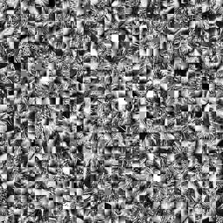
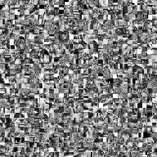
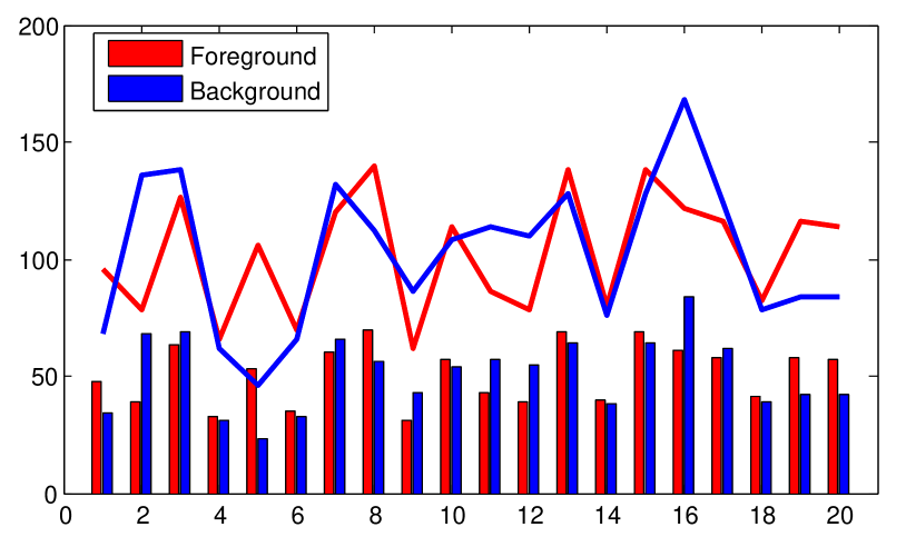
dictionaries for a particular semantic class, and their distributions over $20$-bins. Note that these two dictionaries are not dramatically different. This is not surprising since the dictionary learning process tends to produce a generic basis, as noted by e.g. [21] and many others. Nevertheless, the local variations between the foreground and background distributions still exhibit notable difference.

3.3 Grouped Multitask Lasso and Figure-Ground Separation

Over-segmentation and dictionary learning essentially provide input for multitask Lasso in this part. Sparsity related techniques, such as Lasso in Eq. (3), are normally useful for identifying a subset of most relevant features amongst a redundant collection (shortly known as feature selection). Recent developments have extended Lasso into grouped setting (the Group Lasso [19], or GL), and multitask setting (the MultiTask Lasso [18, 20], or MTL). GL is designed to achieve group sparsity of variable selection with respect to some pre-defined variable groups, and is formulated as

$$\min_{\bm{\alpha}}\|\mathbf{y}-\mathbf{D}\bm{\alpha}\|_{2}^{2}+\lambda\sum_{g=1}^{G}\|\bm{\alpha}_{\mathcal{I}_{g}}\|_{2},$$ (5)

where $\mathcal{I}_{g}$ is the index set of variable(s) belonging to the $g^{th}$ group, for $g=1,\cdots,G$. On the other hand, MTL aims to obtain the same sparsity pattern across tasks. Assuming we are considering $K$ tasks together, and superscript (such as $\mathbf{y}^{\left(k\right)}$) identifies a particular task. We have the objective

$$\min_{\bm{\Omega}}\;\sum_{k=1}^{K}\|\mathbf{y}^{\left(k\right)}-\sum_{j=1}^{n}\omega_{j}^{\left(k\right)}\mathbf{d}_{j}^{\left(k\right)}\|_{2}^{2}+\lambda\sum_{j=1}^{n}\|\bm{\omega}_{j}\|_{q},$$ (6)

where $\mathbf{d}_{j}^{\left(k\right)}$ is the $j^{th}$ basis vector for the $k^{th}$ task, and $n$ is the number of features (size of the dictionary) as defined in last part. Moreover, $\bm{\omega}_{j}=\left(\omega_{j}^{\left(1\right)},\cdots,\omega_{j}^{\left(K\right)}\right)^{\rm T}$ is the vector of all coefficients for the $j^{th}$ feature across different tasks, and $\bm{\Omega}=\left(\bm{\omega}_{1},\cdots,\bm{\omega}_{n}\right)^{\rm T}$. In [18, 20], the $q$-norm for the coefficients is taken as the sup-norm, i.e. $\|\bm{\omega}_{j}\|_{\infty}=\max_{k}|\omega_{j}^{\left(k\right)}|$. We argue that other valid norms can also be taken, esp. the $\ell_{2}$ norm. Taking summation of $\ell_{2}$ norm as the penalization term not only effectively helps combine MTL and GL as can be shortly seen, but results in considerable computational saving as discussed below.

For our particular problem, we want to use the same dictionary $\mathbf{D}=\left(\mathbf{d}_{1},\cdots,\mathbf{d}_{n}\right)$ (concatenation of dictionaries of different object classes, including both foreground and background ones) learned from last part, and reconstruct local patches within each segmented region simultaneously to identify if the region belongs to the object or the background. Hence we drop the superscript for the dictionary straight away and meanwhile choose the $\ell_{2}$ norm. Then the objective we need to optimize reduces to

$$\min_{\bm{\Omega}}\;\sum_{k=1}^{K}\|\mathbf{y}^{\left(k\right)}-\sum_{j=1}^{n}\omega_{j}^{\left(k\right)}\mathbf{d}_{j}\|_{2}^{2}+\lambda\sum_{j=1}^{n}\|\bm{\omega}_{j}\|_{2}.$$ (7)

If we further enforce group sparsity as in GL, across tasks our group reconstruction coefficients will take sub-matrices of the matrix $\bm{\Omega}$. Hence the ultimate formulation will be

$$\min_{\bm{\Omega}}\;\sum_{k=1}^{K}\|\mathbf{y}^{\left(k\right)}-\sum_{j=1}^{n}\omega_{j}^{\left(k\right)}\mathbf{d}_{j}\|_{2}^{2}+\lambda\sum_{g=1}^{G}\|\bm{\Omega}_{\mathcal{I}_{g}}\|_{F},$$ (8)

where $\|\cdot\|_{F}$ is the Frobenius norm for matrices, and $\mathcal{I}_{g}$ takes similar roles as in Eq. (5).

Eq. (8) can be solved by (batch-mode) clockwise coordinate descent as in [20], with a considerably large number of iterations. Instead, we turn the regularization into a constraint and arrive at

$$\min_{\bm{\Omega}}\;\sum_{k=1}^{K}\|\mathbf{y}^{\left(k\right)}-\sum_{j=1}^{n}\omega_{j}^{\left(k\right)}\mathbf{d}_{j}\|_{2}^{2}\;\text{s.t.}\;\sum_{g=1}^{G}\|\bm{\Omega}_{\mathcal{I}_{g}}\|_{F}\leq C,$$ (9)

where $C$ is a constraint parameter dual to the original regularization parameter $\lambda$. By employing matrix notations for $\mathbf{Y}=\left(\mathbf{y}^{\left(1\right)},\cdots,\mathbf{y}^{\left(K\right)}\right)$ in addition to $\mathbf{D}$ and $\bm{\Omega}$, the objective can be written as

$$\min_{\bm{\Omega}}\;\bm{\Omega}^{\rm T}\mathbf{D}^{\rm T}\mathbf{D}\bm{\Omega}-2\mathbf{Y}^{\rm T}\mathbf{D}\bm{\Omega}\;\text{s.t.}\;\sum_{g=1}^{G}\|\bm{\Omega}_{\mathcal{I}_{g}}\|_{F}\leq C.$$ (10)

The following definitions and proposition will be important for numerically solving the optimization.

Definition 1 (Mixed $\ell_{p,q}$-Norm).

For a vector $\mathbf{x}\in\mathbb{R}^{n}$ and a set of disjoint index set $\left\{\mathcal{I}_{g}\right\}_{g=1}^{G}$ such that $\cup_{g}\mathcal{I}_{g}=\left\{1,\cdots,n\right\}$. The $\ell_{p,q}$-norm for $\mathbf{x}$ is defined as $\|\mathbf{x}\|_{p,q}=\left(\sum_{g}\|\mathbf{x}_{\mathcal{I}_{g}}\|_{q}^{p}\right)^{1/p}$, where $\mathbf{x}_{\mathcal{I}_{g}}$ is the tuple consisting of the elements over indexes $\mathcal{I}_{g}$.

Definition 2 ($\ell_{p,q}$-Norm Balls).

$\mathcal{C}=\left\{\mathbf{x}|\|\mathbf{x}\|_{p,q}\leq\tau\right\}$ is the $\ell_{p,q}$-norm ball of radius $\tau$.

Proposition 3 (Projection onto an $\ell_{1,2}$-Norm Ball of Radius $\tau$ [29]).

For a vector $\mathbf{x}\in\mathbb{R}^{n}$ and a set of disjoint index set $\left\{\mathcal{I}_{g}\right\}_{g=1}^{G}$ such that $\cup_{g}\mathcal{I}_{g}=\left\{1,\cdots,n\right\}$. The Euclidean projection $\mathcal{P}_{\mathcal{C}}\left(\mathbf{x}\right)$ onto the $\ell_{1,2}$-norm ball of radius $\tau$ is given by

$$\widetilde{\mathbf{x}_{\mathcal{I}_{g}}}=\mathop{\rm sgn}\left(\mathbf{x}_{\mathcal{I}_{g}}\right)\max\left(0,\|\mathbf{x}_{\mathcal{I}_{g}}\|_{2}-\lambda\right),$$ (11)

where $\mathop{\rm sgn}\left(\mathbf{z}\right)$ is the signum function defined over the vector $\mathbf{z}$ as $\mathop{\rm sgn}\left(\mathbf{z}\right)=\mathbf{z}/\|\mathbf{z}\|_{2}$, and $\lambda$ recursively defined over subset of the index set $\left\{\mathcal{I}_{g}\right\}_{g=1}^{G}$ as $\mathcal{I}_{\lambda}=\left\{j\in\left(1,\cdots,G\right)|\|\mathbf{x}_{\mathcal{I}_{j}}\|_{2}>\lambda\right\}$ and the constraint that $\sum_{j\in\mathcal{I}_{\lambda}}\left(\|\mathbf{x}_{\mathcal{I}_{j}}\|_{2}-\lambda\right)=\tau$.

$\lambda$ in the proposition can be solved efficiently [30], and hence the projection. The $\ell_{1,2}$-constrained quadratic optimization in Eq. (10) has simple analytic gradients, and the constraint is a $\ell_{1,2}$-norm ball with projection rule as discussed above. Hence we can employ the projected gradient method for convex optimization [31] as described in Algorithm 1.

Given $\mathbf{D}$, $\mathbf{Y}$, $C$, $\left\{\mathcal{I}_{g}\right\}_{g=1}^{G}$, $\eta$. Set $\bm{\Omega}^{\left(0\right)}$, $k\leftarrow 0$

while not Converged do

       // gradient descent

       $\bm{\Omega}^{\left(k+1\right)}=\bm{\Omega}^{\left(k\right)}-\eta\left(\mathbf{D}^{T}\mathbf{D}\bm{\Omega}^{\left(k\right)}-\mathbf{D}^{T}\mathbf{Y}\right)$

       // vectorize submatrices

       for $g=1$ to $G$ do

             $\bm{\beta}_{g}$=$\text{vectorize}\left(\bm{\Omega}_{\mathcal{I}_{g}}^{\left(k+1\right)}\right)$

      $\bm{\beta}=\left(\bm{\beta}_{1}^{T};\cdots;\bm{\beta}_{G}^{T}\right)$

       // projection

       Solve $\lambda$

       for $g=1$ to $G$ do

             $\widetilde{\bm{\beta}_{g}}=\mathop{\rm sgn}\left(\bm{\beta}_{g}\right)\max\left(0,\|\bm{\beta}_{g}\|_{2}-\lambda\right)$ ;

             $\bm{\Omega}_{\mathcal{I}_{g}}^{\left(k+1\right)}=\text{devectorize}\left(\widetilde{\bm{\beta}_{g}}\right)$

      

Algorithm 1 Group-Multitask Lasso Algorithm

The convergence is typically within 50 iterations with the above projected gradient method. Upon completion, we use the results to perform figure-ground separation. To this end, both the reconstruction error and the reconstruction coefficients can be used. We find slightest difference for them to distinguish between the object and background, and hence we stick to the reconstruction coefficients for simplicity. We directly compare the sum of reconstruction coefficients within each semantic group (foreground/background) to arrive at the figure-ground separation. We note that we have scaled the dictionary elements such that every feature vector has unity $\ell_{2}$ norm, and hence there should not be cross-scale problem associated with the reconstruction coefficients.

(a) Input Image

(b) Over-Segmentation

(c) FG Map-MTL

(d) FG Map-Lasso

Figure 4: The figure-ground map produced by segmentation-based GMTL vs. segmentation-based voting of patch-wise Lasso. GMTL-based method produces better results.

Figure 4 presents one group of example results on figure-ground separation. Notice that the separation produced by this GMTL step (Figure 4c) is not perfect, and is often dependent on the over-segmentation quality. Nevertheless, as compared to the results produced by patch-wise individual Lasso (Figure 4d), the former results are much better. This has illustrated the benefit of using GMTL for discrimination.

3.4 Image Matting and Further Processing

Image matting as mentioned before is widely used for image editing and other arts production applications. Mathematically, matting involves the simultaneous estimation of the foreground image $\mathbf{F}_{z}$ ($z$ denotes the pixel position) and the background image $\mathbf{B}_{z}$ together with the alpha matte $\bm{\alpha}_{z}$, given the observed image $\mathbf{I}_{z}$, and the matting equation

$$\mathbf{I}_{z}=\alpha_{z}\mathbf{F}_{z}+\left(1-\alpha_{z}\right)\mathbf{B}_{z}.$$ (12)

Matting is a typical inverse problem, and need additional constraints or regularization to be solvable. Most existing technique requires significant manual inputs which is undesirable for our current work. Several recent algorithms need only sparse user scribbles as inputs and even provide closed-form solutions [15].

We choose to use [15] to refine the figure-ground separation map obtained from GMTL, and treat the map (fractional-values at the boundaries) as the scribbled sparse alpha matte. The effectiveness of this novel employment of matting is confirmed by our empirical results (in experiment part). The solution of GMTL for each segment region can be used for SR reconstruction. In addition, we observe that following the patch-wise sparse reconstruction as discussed in [10] provides additional performance gains. Furthermore, other image processing techniques can also be applied to the background region, leading to various visual applications (as shown in Figure 1 and the upcoming Figure 5).

4 Experiments and Discussions

4.1 Dataset Preparation

We select images of five object categories: cow, horse, sheep, cat, and dog from the VOC2009 segmentation dataset and the MSRC object class recognition dataset (version 2), respectively. These datasets are suitable for our purpose of object/background dictionaries training, because they provide pixel-level object/background segmentation groundtruth. We choose animal images to work with more diversity in textures. For each selected dataset, 15 images (about $10\%$ of the total) across all $5$ categories are used for testing, and the remaining for training.

Each training image and its down-sampled version (by the desired magnification factor, typically 3) constitute a high-/low-resolution image pair. $50,000$ patches (with typical size $3\times 3$ pixels w.r.t. the low-resolution image) for the object and the background respectively are then sampled from the training pairs, with the aid of the available groundtruth segmentation. For patch representation, we follow [10] and use the first-order and second-order derivatives as features. The $1$-D filters used for feature extraction are

$$\mathbf{f}_{1}=\left[-1,0,1\right],\mathbf{f}_{2}=\mathbf{f}_{1}^{\rm T},\mathbf{f}_{3}=\left[1,0,-2,0,1\right],\mathbf{f}_{4}=\mathbf{f}_{3}^{\rm T}.$$

Joint dictionary learning as described in Sec. 3.2 is then performed for each category class and its corresponding background, over the sampled patches. Each dictionary contains $1024$ basis patches.

4.2 Figure-Ground Separation and Matting

Based on the learned dictionaries, and the over-segmentation for an input image, the GMTL algorithm figures out the figure-ground separation based on the reconstruction coefficient vectors for each image segment. Several example output maps by this procedure is included in Figure 5 (Group $C$ ). For comparison, we have also generated maps based on the voting of patch-wise reconstruction coefficients within each segment (single Lasso over each patch, and then voting within a segment, Figure 5, Group $B$). It is obvious that often GMTL produces more reliable object regions than the other way. This success is largely due to the joint solution to figure-ground separation within one segment, using the proposed GMTL technique. On the other hand, even GMTL often produces object map with fragmented boundaries or parts as evident from the examples. This is where matting comes into play. We apply our matting scheme as discussed in Sec-3.4 (results in Figure 5, Group $D$). Visual investigation suggests that matting does enhance the object boundaries much, notably at regions e.g. the cow horns, the dogs’ bodies and heads.

4.3 SR and Other Visual Applications

Figure 5: Selective SR and various visual applications. These are four comprehensive examples for demonstrating the system with the notations. $G$: input image, $A$: Over-segmentation map, $B$: patch-wise figure-ground voting map within segments, $C$: GMTL-based figure-ground map, $D$: $C$ after matting, $E$ and $F$: special visual effects, $G$ and $F$: original patch and SR reconstructed patch. (For better view, please refer to the electronic version. Please zoom in to see the special effects.)

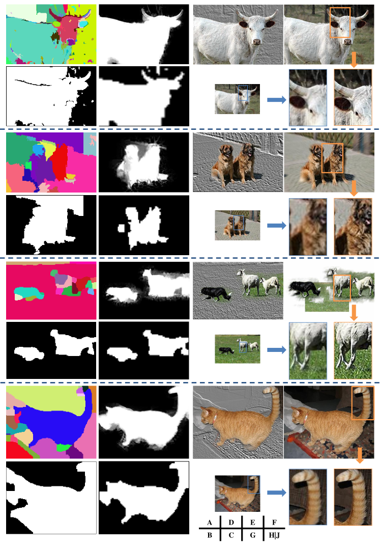
The SR reconstruction is hence based on the matted map instead of the original. Figure 5 compares several of the low-resolution textured patches/regions with that produced by our SR (Group $H$ vs. $J$). The reconstructed ones often contain significant more details than the original. Moreover, several possible visual effects by further processing the backgrounds or/and the objects are shown in Figure 5 (Group $E$ and $F$).

5 Conclusions and Future Work

In this paper we employ and integrate several state-of-the-art methods in recent vision, learning, and graphics research, and build an SR system with selectivity that effectively jointly solves figure-ground separation and SR reconstruction. It is exciting to work along the classic over-segmentation algorithm with the sophisticated sparse coding and multitask Lasso techniques to achieve learning-based figure-ground separation. Equally exciting is the matting technique from graphics research that can effectively enhance the separation, and help us generate good SR reconstruction and fancy visual applications. We plan to further investigate the possibility of generic semantic class identification with the same setting.

6 Reference

References

- Park et al. [2003] S. C. Park, M. K. Park, M. G. Kang, Super-resolution image reconstruction: a technical overview, Signal Processing Magazine, IEEE 20 (2003) 21 – 36.
- Tsai and Huang [1984] R. Tsai, T. Huang, Multiple frame image restoration and registration, Computer Vision and Image Processing 1 (1984) 317–339.
- Baker [2002] K. T. Baker, S., Limits on super-resolution and how to break them, Pattern Analysis and Machine Intelligence, IEEE Transactions on 24 (2002) 1167 – 1183.
- Lin and Shum [2004] Z. Lin, H.-Y. Shum, Fundamental limits of reconstruction-based superresolution algorithms under local translation, Pattern Analysis and Machine Intelligence, IEEE Transactions on 26 (2004) 83 –97.
- Freeman et al. [2000] W. Freeman, E. Pasztor, O. Carmichael, Learning low-level vision, International Journal of Computer Vision 40 (2000) 25–47.
- Freeman et al. [2002] W. Freeman, T. Jones, E. Pasztor, Example-based super-resolution, IEEE Computer Graphics and Applications (2002) 56–65.
- Baker and Kanade [2000] S. Baker, T. Kanade, Hallucinating faces, in: Automatic Face and Gesture Recognition, pp. 83–89.
- Chang et al. [2004] H. Chang, D.-Y. Yeung, Y. Xiong, Super-resolution through neighbor embedding, in: Proc. IEEE Conf. Computer Vision and Pattern Recognition.
- Ni and Nguyen [2007] K. Ni, T. Nguyen, Image superresolution using support vector regression, Image Processing, IEEE Transactions on 16 (2007) 1596–1610.
- Yang et al. [2008] J. Yang, J. Wright, T. Huang, Y. Ma, Image super-resolution as sparse representation of raw image patches.
- Sun et al. [2003] J. Sun, N. Zheng, H. Tao, H. Shum, Image hallucination with primal sketch priors, in: Proc. IEEE Conference on Computer Vision and Pattern Recognition.
- Jojic et al. [2003] N. Jojic, B. Frey, A. Kannan, Epitomic analysis of appearance and shape, in: Proc. International Conference of Computer Vision.
- Gu et al. [2009] C. Gu, J. Lim, P. Arbeláez, J. Malik, Recognition using regions, in: Proc. IEEE Conference on Computer Vision and Pattern Recognition.
- Wang and Cohen [2007] J. Wang, M. Cohen, Image and video matting: A survey, Foundations and Trends® Computer Graphics. Vision. 3 (2007) 97–175.
- Levin et al. [2008] A. Levin, D. Lischinski, Y. Weiss, A closed-form solution to natural image matting, Pattern Analysis and Machine Intelligence, IEEE Transactions on 30 (2008) 228–242.
- Wright et al. [2009a] J. Wright, A. Yang, A. Ganesh, S. Sastry, Y. Ma, Robust Face Recognition via Sparse Representation, Pattern Analysis and Machine Intelligence, IEEE Transactions on 31 (2009a) 210–227.
- Wright et al. [2009b] J. Wright, Y. Ma, J. Mairal, G. Spairo, T. Huang, S. Yan, Sparse Representation for Computer Vision and Pattern Recognition, submitted to Proc. IEEE (2009b).
- Zhang [2006] J. Zhang, A probabilistic framework for multitask learning, Technical Report, Technical Report (CMU-LTI-06-006). Ph. D. thesis, Carnegie Mellon University, 2006.
- Yuan and Lin [2006] M. Yuan, Y. Lin, Model selection and estimation in regression with grouped variables, Journal. Royal statistical society series B Statistical Methodology 68 (2006) 49.
- Liu et al. [2009] H. Liu, M. Palatucci, J. Zhang, Blockwise coordinate descent procedures for the multi-task lasso, with applications to neural semantic basis discovery, in: Proc. 26th International Conference on Machine Learning.
- Lee et al. [2007] H. Lee, A. Battle, R. Raina, A. Ng, Efficient sparse coding algorithms, Advances in neural information processing systems 19 (2007) 801–808.
- Mairal et al. [2009] J. Mairal, F. Bach, J. Ponce, G. Sapiro, Online dictionary learning for sparse coding, in: Proc. 26th International Conference on Machine Learning.
- Mairal et al. [2008] J. Mairal, F. Bach, J. Ponce, G. Sapiro, A. Zisserman, Discriminative learned dictionaries for local image analysis, in: Proc. IEEE Conference on Computer Vision and Pattern Recognition.
- Harzallah et al. [2009] H. Harzallah, F. Jurie, C. Schmid, Combining efficient object localization and image classification, in: Proc. International Conference of Computer Vision.
- Felzenszwalb and Huttenlocher [2004] P. Felzenszwalb, D. Huttenlocher, Efficient graph-based image segmentation, International Journal of Computer Vision 59 (2004) 167–181.
- Donoho [2006] D. Donoho, For most large underdetermined systems of linear equations the minimal l1-norm solution is also the sparsest solution, Communications on Pure and Applied Mathematics 59 (2006) 797–829.
- Efron et al. [2004] B. Efron, T. Hastie, I. Johnstone, R. Tibshirani, Least angle regression, Annals of statistics (2004) 407–451.
- Friedman et al. [2007] J. Friedman, T. Hastie, H. Höfling, R. Tibshirani, Pathwise coordinate optimization, Annals of Applied Statistics 1 (2007) 302–332.
- Schmidt et al. [2009] M. Schmidt, E. van den Berg, M. Friedlander, K. Murphy, Optimizing costly functions with simple constraints: A limited-memory projected quasi-newton algorithm, in: AI & Statistics.
- Duchi et al. [2008] J. Duchi, S. Shalev-Shwartz, Y. Singer, T. Chandra, Efficient projections onto the -ball for learning in high dimensions, in: Proc. 25th International Conference on Machine learning, pp. 272–279.
- Bertsekas [1999] D. Bertsekas, Nonlinear programming, Athena Scientific, Belmont, MA, 1999.