A Generalized Coupon Collector Problem

Abstract

This paper provides analysis to a generalized version of the coupon collector problem, in which the collector gets d𝑑d coupons each run and he chooses the one that he has the least so far. In the asymptotic case when the number of coupons n𝑛n goes to infinity, we show that on average n​log⁑nd+nd​(mβˆ’1)​log⁑log⁑n+O​(m​n)π‘›π‘›π‘‘π‘›π‘‘π‘š1π‘›π‘‚π‘šπ‘›\frac{n\log n}{d}+\frac{n}{d}(m-1)\log\log{n}+O(mn) runs are needed to collect mπ‘šm sets of coupons. An efficient exact algorithm is also developed for any finite case to compute the average needed runs exactly. Numerical examples are provided to verify our theoretical predictions.

keywords:
Coupon collector problem, expected runs, state-space representation, opportunistic scheduling, wireless communications
\authornames

Weiyu Xu, A. Kevin Tang

\authorone

[Cornell University]Weiyu Xu \addressoneSchool of Electrical and Computer Engineering, Cornell University, Ithaca, NY 14853, USA. Email: wx42@cornell.edu.

\authortwo

[Cornell University]A. Kevin Tang

\addresstwo

School of Electrical and Computer Engineering, Cornell University, Ithaca, NY 14853, USA. Email: atang@ece.cornell.edu.

\ams

60G7060C05

1 Introduction

The classic coupon collector problem asks for the expected number of runs to collect a complete set of n𝑛n different coupons while during each run the collector randomly gets a coupon. The answer is n​Hn𝑛subscript𝐻𝑛nH_{n} where Hn=βˆ‘k=1n1ksubscript𝐻𝑛superscriptsubscriptπ‘˜1𝑛1π‘˜H_{n}=\sum_{k=1}^{n}\frac{1}{k} is the harmonic number [2]. One can further ask for the expected number of runs to collect mπ‘šm complete sets of coupons, which has been addressed by Newman and Shepp [8].

The coupon collector problem and its variants are of traditional and recurrent interest [3, 5, 6, 4, 7]. Besides of their rich theoretical structures and implications, there are various applications of them as well including dynamic resource allocation, hashing and online load balancing [1], to just name a few. In particular, we want to point out that these problems also serve as basic models to analyze delay for opportunistic scheduling in broadcast wireless fading channels [9]. For example, to maximize system throughput, we should serve to the user whose channel condition is the best at every time slot. In order to evaluate performance, one may ask about the expected number of time slots needed for all users to be served at least once. Assuming all channels are i.i.d., then this is equivalent to the classic coupon collector problem.

In this paper, we investigate a natural generalization of the coupon collector problem. Instead of getting one coupon, the collector gets d𝑑d (1≀d≀n1𝑑𝑛1\leq d\leq n) distinct coupons randomly each run and he picks one that so far he has the least. Formally, we denote the number of runs (a β€œrun” often referred to a unit of β€œtime slot” or simply a unit of β€œtime” in this paper) that are used to collect mπ‘šm sets of coupons as Dm,ndsubscriptsuperscriptπ·π‘‘π‘šπ‘›D^{d}_{m,n} and we are interested in characterizing the mean value of this random variable Dm,ndsubscriptsuperscriptπ·π‘‘π‘šπ‘›D^{d}_{m,n} especially in the asymptotic region when n𝑛n is large. Clearly, when d=1𝑑1d=1, we go back to the classic cases; when d=n𝑑𝑛d=n, there is no randomness and Dm,nn=m​nsubscriptsuperscriptπ·π‘›π‘šπ‘›π‘šπ‘›D^{n}_{m,n}=mn. In the scheduling transmission context we just discussed, d𝑑d can be viewed as a parameter to control the tradeoff between efficiency (high throughput) and fairness among all users with d=1𝑑1d=1 purely focusing on efficiency while d=n𝑑𝑛d=n giving out perfect fairness.

In the remaining part of this paper, we first briefly review existing related results in Section 2. Although they are all special cases of the general problem, the techniques used to derive them cannot be applied directly to the general case. Instead, we develop a new technique to characterize E​(Dm,nd)𝐸subscriptsuperscriptπ·π‘‘π‘šπ‘›E(D^{d}_{m,n}) and provide upper and lower bounds for E​(Dm,nd)𝐸subscriptsuperscriptπ·π‘‘π‘šπ‘›E(D^{d}_{m,n}) in Section 3 and Section 4. An asymptotic analysis shows that the upper bound and lower bound match in the asymptotic regime of nβ†’βˆžβ†’π‘›n\rightarrow\infty in Section 5 . Furthermore, for any finite n𝑛n, an algorithm is motivated and proposed in Section 6 to calculate E​(Dm,nd)𝐸subscriptsuperscriptπ·π‘‘π‘šπ‘›E(D^{d}_{m,n}) exactly. Finally, we use numerical examples to validate our theoretical predictions in section 7.

2 Existing Results

The existing results on special cases are listed below. If d=1𝑑1d=1, then the problem is solved for all mβ‰₯1π‘š1m\geq 1. If d>1𝑑1d>1, then only the m=1π‘š1m=1 case is known.

  • β€’

    d=1,m=1formulae-sequence𝑑1π‘š1d=1,m=1 ([2]). It is clear that the number of runs needed to obtain (i+1)𝑖1(i+1)-th coupon after obtaining the i𝑖i-th one follows a geometric distribution with parameter nβˆ’in𝑛𝑖𝑛\frac{n-i}{n}. Therefore,

    E​(D1,n1)=n​Hn=nβ€‹βˆ‘k=1n1k𝐸subscriptsuperscript𝐷11𝑛𝑛subscript𝐻𝑛𝑛superscriptsubscriptπ‘˜1𝑛1π‘˜E(D^{1}_{1,n})=nH_{n}=n\sum_{k=1}^{n}\frac{1}{k} (1)

    For large n𝑛n,

    E​(D1,n1)=n​log⁑n+n​O​(1)𝐸subscriptsuperscript𝐷11𝑛𝑛𝑛𝑛𝑂1E(D^{1}_{1,n})=n\log n+nO(1) (2)

    One sees that the randomness cost is expressed approximately by a factor log⁑n𝑛\log n.

  • β€’

    d=1,mβ‰₯1formulae-sequence𝑑1π‘š1d=1,m\geq 1 ([8]).

    E​(Dm,n1)=nβ€‹βˆ«0∞(1βˆ’(1βˆ’Sm​(t)​eβˆ’t)n)​𝑑t𝐸subscriptsuperscript𝐷1π‘šπ‘›π‘›superscriptsubscript01superscript1subscriptπ‘†π‘šπ‘‘superscript𝑒𝑑𝑛differential-d𝑑E(D^{1}_{m,n})=n\int_{0}^{\infty}(1-(1-S_{m}(t)e^{-t})^{n})dt (3)

    where Sm​(t)=βˆ‘k=0mβˆ’1tkk!subscriptπ‘†π‘šπ‘‘superscriptsubscriptπ‘˜0π‘š1superscriptπ‘‘π‘˜π‘˜S_{m}(t)=\sum_{k=0}^{m-1}\frac{t^{k}}{k!}.

    For fixed mπ‘šm and large n𝑛n,

    E​(Dm,n1)=n​log⁑n+n​(mβˆ’1)​log⁑log⁑n+n​O​(1).𝐸subscriptsuperscript𝐷1π‘šπ‘›π‘›π‘›π‘›π‘š1𝑛𝑛𝑂1E(D^{1}_{m,n})=n\log n+n(m-1)\log\log n+nO(1). (4)

    It is interesting to note that although collecting the first set of coupons needs about n​log⁑n𝑛𝑛n\log n runs, all later sets only need n​log⁑log⁑n𝑛𝑛n\log\log n runs per set.

  • β€’

    dβ‰₯1,m=1formulae-sequence𝑑1π‘š1d\geq 1,m=1 ([9]). This has applications in the scheduling of data packets transmission over wireless channels. Here

    E​(D1,nd)=βˆ‘i=0nβˆ’111βˆ’(id)(nd),𝐸subscriptsuperscript𝐷𝑑1𝑛superscriptsubscript𝑖0𝑛111binomial𝑖𝑑binomial𝑛𝑑E(D^{d}_{1,n})=\sum_{i=0}^{n-1}\frac{1}{1-\frac{\binom{i}{d}}{\binom{n}{d}}}, (5)

    where (id)=0binomial𝑖𝑑0\binom{i}{d}=0 if i<d𝑖𝑑i<d.

    For fixed mπ‘šm and large n𝑛n,

    E​(D1,nd)∼1d​n​log⁑n.similar-to𝐸subscriptsuperscript𝐷𝑑1𝑛1𝑑𝑛𝑛E(D^{d}_{1,n})\sim\frac{1}{d}n\log n. (6)

    This shows that for the m=1π‘š1m=1 case, allowing choosing d𝑑d coupons randomly each time decreases the expected number of runs and most of the decreases occurs from d=1𝑑1d=1 to d=2𝑑2d=2.

  • β€’

    dβ‰₯1,mβ‰₯1formulae-sequence𝑑1π‘š1d\geq 1,m\geq 1. In the mentioned context of scheduling, if a transmitter wants to send mπ‘šm packets to each of the n𝑛n users, but each time he can only transmits one packet to one user chosen from the d𝑑d users who have the best wireless communication channels. Due to the time varying nature of the wireless channels, it is natural to assume that for each time index, the d𝑑d users who have the best communication channels are uniformly distributed among the n𝑛n users. So E​(Dm,nd)𝐸superscriptsubscriptπ·π‘šπ‘›π‘‘E(D_{m,n}^{d}) gives an estimate on the total delay in delivering these mπ‘šm packets, and, in this paper, we will offer a characterization of E​(Dm,nd)𝐸superscriptsubscriptπ·π‘šπ‘›π‘‘E(D_{m,n}^{d}).

3 Lower Bound on E​(Dm,nd)𝐸superscriptsubscriptπ·π‘šπ‘›π‘‘E(D_{m,n}^{d})

We will first lower bound E​(Dm,nd)𝐸superscriptsubscriptπ·π‘šπ‘›π‘‘E(D_{m,n}^{d}) by considering a different coupon collecting process. In this new process, each time we uniformly select d𝑑d distinct coupons out of n𝑛n coupons, and instead of keeping only one coupon out of these d𝑑d selected coupons, we would keep all these d𝑑d coupons. Apparently, the expected time of collecting mπ‘šm sets of coupons in this way will be no larger than the process which only keeps one coupon a time.

However, it is not so straightforward to directly get a estimate for this new process. This motivates us to consider another process in which each time, one will collect d𝑑d uniformly, independently chosen (allowing repeating) coupons and keep all of them. This process stops when mπ‘šm sets of coupons are fully collected.

Lemma 3.1

Let t1subscript𝑑1t_{1} be the expected time to collected mπ‘šm sets of coupons for the process in which each time d𝑑d uniformly chosen distinct coupons are kept. Let t2subscript𝑑2t_{2} be the expected time to collected mπ‘šm sets of coupons for the process in which each time d𝑑d uniformly chosen (allowing repetition) coupons are kept. Then

t1β‰₯(nd)nd​t2.subscript𝑑1binomial𝑛𝑑superscript𝑛𝑑subscript𝑑2t_{1}\geq\frac{\binom{n}{d}}{n^{d}}t_{2}. (7)
Proof 3.2

We simulate the process of choosing d𝑑d distinct coupons through an expurgated process of choosing d𝑑d independent coupons (allowing repetition). If the d𝑑d coupons we independently choose (allowing repeating) are not distinct, we will discard this group of d𝑑d coupons; if they are all distinct d𝑑d coupons, we will keep them. The kept coupons from expurgated process follow the same distribution as the chosen d𝑑d distinct coupons. However, the expected time for one to get a group of d𝑑d distinct coupons is clearly nd(nd)superscript𝑛𝑑binomial𝑛𝑑\frac{n^{d}}{\binom{n}{d}}. So in the worst case, t2≀nd(nd)​t1subscript𝑑2superscript𝑛𝑑binomial𝑛𝑑subscript𝑑1t_{2}\leq\frac{n^{d}}{\binom{n}{d}}t_{1}. Β  Β β–‘β–‘\Box

In summary, in order to give a lower bound on E​(Dm,nd)𝐸superscriptsubscriptπ·π‘šπ‘›π‘‘E(D_{m,n}^{d}), we will first need a lower bound on t2subscript𝑑2t_{2} for the process of keeping d𝑑d uniformly randomly chosen coupons (allowing reptition). To do this, we follow the approach of generating functions in [8].

Let pisubscript𝑝𝑖p_{i} be the probability of failure of obtaining mπ‘šm sets of coupons when we have kept i𝑖i coupons. Let Px1,β‹―,xnsubscript𝑃subscriptπ‘₯1β‹―subscriptπ‘₯𝑛P_{x_{1},\cdots,x_{n}} be a power series and let {Px1,β‹―,xn}subscript𝑃subscriptπ‘₯1β‹―subscriptπ‘₯𝑛\{P_{x_{1},\cdots,x_{n}}\} be the power series when all terms having all exponents β‰₯mabsentπ‘š\geq m have been removed. By these notations,

t2=βˆ‘j=0∞pd​j,subscript𝑑2superscriptsubscript𝑗0subscript𝑝𝑑𝑗t_{2}=\sum_{j=0}^{\infty}p_{dj},

and

pd​j={(x1+β‹―+xn)d​j}nd​j,subscript𝑝𝑑𝑗superscriptsubscriptπ‘₯1β‹―subscriptπ‘₯𝑛𝑑𝑗superscript𝑛𝑑𝑗p_{dj}=\frac{\{(x_{1}+\cdots+x_{n})^{dj}\}}{n^{dj}},

with x1,β‹―,xnsubscriptπ‘₯1β‹―subscriptπ‘₯𝑛{x_{1},\cdots,x_{n}} all equal to 111.

In addition, we know

E​(Dm,n1)=βˆ‘q=0dβˆ’1βˆ‘j=0∞pd​j+q=nβ€‹βˆ«0∞(1βˆ’(1βˆ’Sm​(t)​eβˆ’t)n)​𝑑t,𝐸subscriptsuperscript𝐷1π‘šπ‘›superscriptsubscriptπ‘ž0𝑑1superscriptsubscript𝑗0subscriptπ‘π‘‘π‘—π‘žπ‘›superscriptsubscript01superscript1subscriptπ‘†π‘šπ‘‘superscript𝑒𝑑𝑛differential-d𝑑E(D^{1}_{m,n})=\sum_{q=0}^{d-1}\sum_{j=0}^{\infty}p_{dj+q}=n\int_{0}^{\infty}(1-(1-S_{m}(t)e^{-t})^{n})dt,

where Sm​(t)=βˆ‘k=0mβˆ’1tkk!subscriptπ‘†π‘šπ‘‘superscriptsubscriptπ‘˜0π‘š1superscriptπ‘‘π‘˜π‘˜S_{m}(t)=\sum_{k=0}^{m-1}\frac{t^{k}}{k!} [8].

We also notice that pisubscript𝑝𝑖p_{i} is nonincreasing as i𝑖i grows, so

t2subscript𝑑2\displaystyle t_{2} =\displaystyle= βˆ‘j=0∞pd​jβ‰₯(βˆ‘j=0∞pj)/dsuperscriptsubscript𝑗0subscript𝑝𝑑𝑗superscriptsubscript𝑗0subscript𝑝𝑗𝑑\displaystyle\sum_{j=0}^{\infty}p_{dj}\geq(\sum_{j=0}^{\infty}p_{j})/d
β‰₯\displaystyle\geq nβ€‹βˆ«0∞(1βˆ’(1βˆ’Sm​(t)​eβˆ’t)n)​𝑑t/d.𝑛superscriptsubscript01superscript1subscriptπ‘†π‘šπ‘‘superscript𝑒𝑑𝑛differential-d𝑑𝑑\displaystyle n\int_{0}^{\infty}(1-(1-S_{m}(t)e^{-t})^{n})dt/d.

So by (7), we know

E​(Dm,nd)β‰₯(nd)nd​(E​(Dm,n1)/d).𝐸superscriptsubscriptπ·π‘šπ‘›π‘‘binomial𝑛𝑑superscript𝑛𝑑𝐸superscriptsubscriptπ·π‘šπ‘›1𝑑E(D_{m,n}^{d})\geq\frac{\binom{n}{d}}{n^{d}}\left(E(D_{m,n}^{1})/d\right).

4 Upper Bound on E​(Dm,nd)𝐸superscriptsubscriptπ·π‘šπ‘›π‘‘E(D_{m,n}^{d})

In this section, we will upper bound the expected time of collecting mπ‘šm complete sets of coupons. To achieve this, we will upper bound the expected time for collecting mπ‘šm complete sets of coupons in a suboptimal process. In this new process, each time, we will uniformly and independently choose d𝑑d coupons (allowing repetition). Among this group of d𝑑d coupons, we will start looking at them one by one. If the i𝑖i-th (1≀i≀d1𝑖𝑑1\leq i\leq d) coupon is the first such a coupon that we so far have fewer than mπ‘šm copies, then we will keep this i𝑖i-th coupon and discard the remaining (dβˆ’i)𝑑𝑖(d-i) coupons.

First of all, we observe that d𝑑d distinct coupons are favorable in terms of minimizing the collection time compared with d𝑑d coupons with possible repeating.

Theorem 4.1

The minimized expected time of collecting mπ‘šm sets of coupons, when each time the coupon collector is given d𝑑d uniformly chosen distinct coupons but is only allowed to keep 111 coupon, is no bigger than the minimized expected time of collecting mπ‘šm set of coupons, when each time the coupon collector is given d𝑑d uniformly chosen coupons (allowing repeating) but is only allowed to keep 111 coupon.

Proof 4.2

Apparently, when the coupon collector is given d𝑑d distinct coupons, he has more choices in making his decisions. Β  Β β–‘β–‘\Box

Secondly, we show that it is an optimal strategy for the coupon collector to keep the coupon out of the d𝑑d incoming coupons (whether allowing repetition or not), for which he has the fewest copies.

Theorem 4.3

The expected time of collecting mπ‘šm sets of coupons is minimized when each time, the coupon collector keeps the coupon which he has the fewest so far, if the coupon collector is allowed to keep only 111 out of the d𝑑d offered coupons.

Proof 4.4

Suppose (before the coupon collector finishes collecting all mπ‘šm sets of coupons) among the uniformly chosen d𝑑d (either distinct or allowing repeating) coupons, the j𝑗j-th type of coupon (there are in total n𝑛n types of coupons and 1≀j≀n1𝑗𝑛1\leq j\leq n) is what he has the fewest, say c1subscript𝑐1c_{1} copies. Suppose further that he chooses instead to keep a different type of coupon, say the l𝑙l-th (1≀l≀n1𝑙𝑛1\leq l\leq n, lβ‰ j𝑙𝑗l\neq j) type of coupon, and, for this type of coupon, the coupon collector has already got c2subscript𝑐2c_{2} copies, where c2>c1subscript𝑐2subscript𝑐1c_{2}>c_{1}. Immediately, we know that after keeping the l𝑙l-th type of coupon, we have at least c2+1subscript𝑐21c_{2}+1 copies of l𝑙l-th type of coupons, which satisfies c2+1β‰₯c1+2subscript𝑐21subscript𝑐12c_{2}+1\geq c_{1}+2. We call the resulting state for the kept coupons as A𝐴A, identified by the tuple (c1,c2+1)subscript𝑐1subscript𝑐21(c_{1},c_{2}+1). Otherwise we would just keep the j𝑗j-th type of coupon, then we will have c1+1subscript𝑐11c_{1}+1 coupons of type j𝑗j and c2subscript𝑐2c_{2} coupons of type l𝑙l. We call the resulting state in this case as B𝐡B, identified by the tuple (c1+1,c2)subscript𝑐11subscript𝑐2(c_{1}+1,c_{2}).

Now we argue that to collect mπ‘šm sets of coupons, on average starting from state B𝐡B will take no longer time than starting from state A𝐴A. The main idea is to let the collector starting from B𝐡B follows the strategy of the collector starting from A𝐴A, and do no worse in the expected delay.

Let us consider two coupon collectors, one starting from state A𝐴A and the other starting from state B𝐡B. At each time index, these two collectors get the same d𝑑d coupons. A coupon collector will keep one coupon only if he has fewer than mπ‘šm copies of coupons of that type. Suppose that the coupon collector starting from state A𝐴A follows his optimized β€œkeeping” decision such that his expected time to fully collect mπ‘šm sets of coupons is minimized. Then we let the coupon collector starting from state B𝐡B follow the same decision process as the coupon collector starting from state A𝐴A, until some time index when the coupon collector starting from state A𝐴A decides to keep a coupon of type j𝑗j or type l𝑙l. At that time index, we also let the coupon collector starting from state B𝐡B keep the same type of coupon as the coupon collector starting from state A𝐴A does. Then let {c1β€²,c2β€²}superscriptsubscript𝑐1β€²superscriptsubscript𝑐2β€²\{c_{1}^{\prime},c_{2}^{\prime}\} denote the resulting numbers of kept coupons of type j𝑗j and type l𝑙l, for the collector starting from state A𝐴A; and likewise define {c1β€²β€²,c2β€²β€²}superscriptsubscript𝑐1β€²β€²superscriptsubscript𝑐2β€²β€²\{c_{1}^{\prime\prime},c_{2}^{\prime\prime}\} for the collector starting from state B𝐡B.

Now we can take an inspection of state {c1β€²,c2β€²}superscriptsubscript𝑐1β€²superscriptsubscript𝑐2β€²\{c_{1}^{\prime},c_{2}^{\prime}\} and state {c1β€²β€²,c2β€²β€²}superscriptsubscript𝑐1β€²β€²superscriptsubscript𝑐2β€²β€²\{c_{1}^{\prime\prime},c_{2}^{\prime\prime}\}. There are two scenarios to discuss separately.

In the first scenario, c2=c1+1subscript𝑐2subscript𝑐11c_{2}=c_{1}+1 and it is the coupon of type j𝑗j that the coupon collector decides to keep at that time index. Then {c1β€²,c2β€²}={c1+1,c2+1}superscriptsubscript𝑐1β€²superscriptsubscript𝑐2β€²subscript𝑐11subscript𝑐21\{c_{1}^{\prime},c_{2}^{\prime}\}=\{c_{1}+1,c_{2}+1\} and {c1β€²β€²,c2β€²β€²}={c1+2,c2}={c2+1,c1+1}superscriptsubscript𝑐1β€²β€²superscriptsubscript𝑐2β€²β€²subscript𝑐12subscript𝑐2subscript𝑐21subscript𝑐11\{c_{1}^{\prime\prime},c_{2}^{\prime\prime}\}=\{c_{1}+2,c_{2}\}=\{c_{2}+1,c_{1}+1\}. Apparently {c1β€²,c2β€²}superscriptsubscript𝑐1β€²superscriptsubscript𝑐2β€²\{c_{1}^{\prime},c_{2}^{\prime}\} and {c1β€²β€²,c2β€²β€²}superscriptsubscript𝑐1β€²β€²superscriptsubscript𝑐2β€²β€²\{c_{1}^{\prime\prime},c_{2}^{\prime\prime}\} are just the permutations of each other, and so by symmetry, the optimized time from these two new states to the completion of collecting mπ‘šm sets of coupons will be the same.

In the second scenario, we have βˆ’c1β€²+c2β€²>βˆ’c1β€²β€²+c2β€²β€²β‰₯0superscriptsubscript𝑐1β€²superscriptsubscript𝑐2β€²superscriptsubscript𝑐1β€²β€²superscriptsubscript𝑐2β€²β€²0-c_{1}^{\prime}+c_{2}^{\prime}>-c_{1}^{\prime\prime}+c_{2}^{\prime\prime}\geq 0. In this scenario, we update state A𝐴A as {c1β€²,c2β€²}superscriptsubscript𝑐1β€²superscriptsubscript𝑐2β€²\{c_{1}^{\prime},c_{2}^{\prime}\} and update state B𝐡B as {c1β€²β€²,c2β€²β€²}superscriptsubscript𝑐1β€²β€²superscriptsubscript𝑐2β€²β€²\{c_{1}^{\prime\prime},c_{2}^{\prime\prime}\}; and then construct an iterative process of evolving states A𝐴A and B𝐡B as follows. (To keep the notations consistent, at the beginning of a new iteration, we always represent state A𝐴A and state B𝐡B by {c1β€²,c2β€²}superscriptsubscript𝑐1β€²superscriptsubscript𝑐2β€²\{c_{1}^{\prime},c_{2}^{\prime}\} and {c1β€²β€²,c2β€²β€²}superscriptsubscript𝑐1β€²β€²superscriptsubscript𝑐2β€²β€²\{c_{1}^{\prime\prime},c_{2}^{\prime\prime}\}, even though they are different numbers than in previous iterations. We also remark that during these iterations, c1β€²,c2β€²,c1β€²β€²,c2β€²β€²superscriptsubscript𝑐1β€²superscriptsubscript𝑐2β€²superscriptsubscript𝑐1β€²β€²superscriptsubscript𝑐2β€²β€²c_{1}^{\prime},c_{2}^{\prime},c_{1}^{\prime\prime},c_{2}^{\prime\prime} always satisfy the listed constraints (8)-(12), which will be obvious from the iterative process description.)

At the beginning of each iteration, we have two coupon collectors starting from states A𝐴A and B𝐡B respectively. At each time index, the coupon collector starting from state B𝐡B will keep the same type of coupon as the coupon collector starting from state A𝐴A, until some run they keep a coupon of either type j𝑗j or type l𝑙l. Again, we have two cases to consider.

In the first case, c1β€²β€²=c2β€²β€²superscriptsubscript𝑐1β€²β€²superscriptsubscript𝑐2β€²β€²c_{1}^{\prime\prime}=c_{2}^{\prime\prime} and it is the coupon of type j𝑗j that the coupon collectors decide to keep at that time index. After keeping that coupon, we have states {c1β€²+1,c2β€²}superscriptsubscript𝑐1β€²1superscriptsubscript𝑐2β€²\{c_{1}^{\prime}+1,c_{2}^{\prime}\} and {c1β€²β€²+1,c2β€²β€²}superscriptsubscript𝑐1β€²β€²1superscriptsubscript𝑐2β€²β€²\{c_{1}^{\prime\prime}+1,c_{2}^{\prime\prime}\} for the collectors starting from A𝐴A and starting from B𝐡B, respectively. So if c1β€²β€²+1=c2β€²superscriptsubscript𝑐1β€²β€²1superscriptsubscript𝑐2β€²c_{1}^{\prime\prime}+1=c_{2}^{\prime}, then by symmetry, {c1β€²β€²+1,c2β€²β€²}superscriptsubscript𝑐1β€²β€²1superscriptsubscript𝑐2β€²β€²\{c_{1}^{\prime\prime}+1,c_{2}^{\prime\prime}\} and {c1β€²+1,c2β€²}superscriptsubscript𝑐1β€²1superscriptsubscript𝑐2β€²\{c_{1}^{\prime}+1,c_{2}^{\prime}\} are two equivalent states, and we are done (note that c1β€²+c2β€²=c1β€²β€²+c2β€²β€²superscriptsubscript𝑐1β€²superscriptsubscript𝑐2β€²superscriptsubscript𝑐1β€²β€²superscriptsubscript𝑐2β€²β€²c_{1}^{\prime}+c_{2}^{\prime}=c_{1}^{\prime\prime}+c_{2}^{\prime\prime}) ; otherwise, if c1β€²β€²+1<c2β€²superscriptsubscript𝑐1β€²β€²1superscriptsubscript𝑐2β€²c_{1}^{\prime\prime}+1<c_{2}^{\prime}, we update state A𝐴A and B𝐡B as {c1β€²+1,c2β€²}superscriptsubscript𝑐1β€²1superscriptsubscript𝑐2β€²\{c_{1}^{\prime}+1,c_{2}^{\prime}\} and {c2β€²β€²,c1β€²β€²+1}superscriptsubscript𝑐2β€²β€²superscriptsubscript𝑐1β€²β€²1\{c_{2}^{\prime\prime},c_{1}^{\prime\prime}+1\} respectively.

In the second case, after keeping that new coupon of type j𝑗j or type l𝑙l, we simply update state A𝐴A and state B𝐡B respectively to record the new numbers of type j𝑗j and type l𝑙l coupons for these two coupon collectors. Then we go back to the beginning of another iteration.

Note in all these iterations, we always maintain

c1β€²+c2β€²superscriptsubscript𝑐1β€²superscriptsubscript𝑐2β€²\displaystyle c_{1}^{\prime}+c_{2}^{\prime} =\displaystyle= c1β€²β€²+c2β€²β€²,superscriptsubscript𝑐1β€²β€²superscriptsubscript𝑐2β€²β€²\displaystyle c_{1}^{\prime\prime}+c_{2}^{\prime\prime}, (8)
c1β€²superscriptsubscript𝑐1β€²\displaystyle c_{1}^{\prime} ≀\displaystyle\leq c2β€²,superscriptsubscript𝑐2β€²\displaystyle c_{2}^{\prime}, (9)
c1β€²β€²superscriptsubscript𝑐1β€²β€²\displaystyle c_{1}^{\prime\prime} ≀\displaystyle\leq c2β€²β€²,superscriptsubscript𝑐2β€²β€²\displaystyle c_{2}^{\prime\prime}, (10)
c2β€²βˆ’c1β€²superscriptsubscript𝑐2β€²superscriptsubscript𝑐1β€²\displaystyle c_{2}^{\prime}-c_{1}^{\prime} >\displaystyle> c2β€²β€²βˆ’c1β€²β€²,superscriptsubscript𝑐2β€²β€²superscriptsubscript𝑐1β€²β€²\displaystyle c_{2}^{\prime\prime}-c_{1}^{\prime\prime}, (11)
c1β€²,c2β€²,c1β€²β€²,c2β€²β€²superscriptsubscript𝑐1β€²superscriptsubscript𝑐2β€²superscriptsubscript𝑐1β€²β€²superscriptsubscript𝑐2β€²β€²\displaystyle c_{1}^{\prime},c_{2}^{\prime},c_{1}^{\prime\prime},c_{2}^{\prime\prime} ≀\displaystyle\leq m.π‘š\displaystyle m. (12)

Because of this, in each iteration, when the coupon collector starting from A𝐴A can keep a certain type of coupon, the coupon collector starting from state B𝐡B can also keep the same type of coupon.

Because for every iteration, we will increase c1β€²+c2β€²superscriptsubscript𝑐1β€²superscriptsubscript𝑐2β€²c_{1}^{\prime}+c_{2}^{\prime} and c1β€²β€²+c2β€²β€²superscriptsubscript𝑐1β€²β€²superscriptsubscript𝑐2β€²β€²c_{1}^{\prime\prime}+c_{2}^{\prime\prime}, and c1β€²,c2β€²,c1β€²β€²,c2′′≀msuperscriptsubscript𝑐1β€²superscriptsubscript𝑐2β€²superscriptsubscript𝑐1β€²β€²superscriptsubscript𝑐2β€²β€²π‘šc_{1}^{\prime},c_{2}^{\prime},c_{1}^{\prime\prime},c_{2}^{\prime\prime}\leq m, if we iterate the previous processes, we will eventually run into a pair of symmetric states in some iteration for these two coupon collectors.

Since we can always end up in a symmetric state for the two coupon collectors, starting from B𝐡B to collect mπ‘šm sets of coupons will not take longer time than starting from A𝐴A.

Β  Β β–‘β–‘\Box

In fact, the previous arguments can essentially show that starting from a state {c1β€²,c2β€²}superscriptsubscript𝑐1β€²superscriptsubscript𝑐2β€²\{c_{1}^{\prime},c_{2}^{\prime}\} has no bigger expected collection time than from the state {c1β€²β€²,c2β€²β€²}superscriptsubscript𝑐1β€²β€²superscriptsubscript𝑐2β€²β€²\{c_{1}^{\prime\prime},c_{2}^{\prime\prime}\}, if |c1β€²βˆ’c2β€²|<|c1β€²β€²βˆ’c2β€²β€²|superscriptsubscript𝑐1β€²superscriptsubscript𝑐2β€²superscriptsubscript𝑐1β€²β€²superscriptsubscript𝑐2β€²β€²|c_{1}^{\prime}-c_{2}^{\prime}|<|c_{1}^{\prime\prime}-c_{2}^{\prime\prime}| and c1β€²+c2β€²=c1β€²β€²+c2β€²β€²superscriptsubscript𝑐1β€²superscriptsubscript𝑐2β€²superscriptsubscript𝑐1β€²β€²superscriptsubscript𝑐2β€²β€²c_{1}^{\prime}+c_{2}^{\prime}=c_{1}^{\prime\prime}+c_{2}^{\prime\prime}.

At this point, we are ready to present the following upper bound for E​(Dm,nd)𝐸superscriptsubscriptπ·π‘šπ‘›π‘‘E(D_{m,n}^{d}).

Theorem 4.5

Suppose that the coupon collector is given d𝑑d uniformly randomly chosen d𝑑d distinct coupons and he is only allowed to keep one out of these d𝑑d distinct coupons. Then the expected time E​(Dm,nd)≀E​(Dm,n1)d+m​n​(1βˆ’1/d)𝐸superscriptsubscriptπ·π‘šπ‘›π‘‘πΈsuperscriptsubscriptπ·π‘šπ‘›1π‘‘π‘šπ‘›11𝑑E(D_{m,n}^{d})\leq\frac{E(D_{m,n}^{1})}{d}+mn(1-1/d).

Proof 4.6

From Theorem 4.3 and 4.1, we will consider an upper bound on the expected finishing time if each run the coupon collector is given d𝑑d independently chosen coupons (allowing repeating) and he decides to keep only the first β€œuseful” coupon when it is available among the d𝑑d coupons. Here a kept β€œuseful” coupon means this coupon is kept before the coupon collector has mπ‘šm copies of that type of coupon.

The idea of the proof is to upper bound the expected finishing time conditioning on a a specific sequence of kept coupons, until we have mπ‘šm sets of coupons. By a specific sequence of β€œkeeper” coupons, we mean a sequence of kept β€œuseful” coupons, specified in their types and the order of keeping them. We note that a specific sequence of β€œkeeper” coupons contain m​nπ‘šπ‘›mn coupons.

First we make a key observation about the probability that the coupon collector follows a specific sequence of β€œkeeper” coupons. This probability will be the same as the corresponding probability that he follows this specific sequence of kept coupons, in another collection process where each run he is only offered 111 instead of d𝑑d independently, uniformly chosen coupons. This is because, when the coupon collector is offered d𝑑d coupons, he still checks them one by one and only keeps the first one that is β€œuseful”.

Now, conditioning on a specific sequence of kept coupons, we are interested in the expected time to collect that sequence. Suppose that right after the rπ‘Ÿr-th coupon in this β€œkeeper” sequence has just been kept, there are s𝑠s types of coupons for which the coupon collector have mπ‘šm copies. We then want to know what is the expected number of runs needed to collect the next (r+1)π‘Ÿ1(r+1)-th β€œkeeper” coupon, conditioning on the whole β€œkeeper” coupon sequence is known.

Through the conditional event that the β€œkeeper” sequence has already specified, it is a standard exercise to show that the average time the coupon collector takes to collect the (r+1)π‘Ÿ1(r+1)-th β€œkeeper” coupon will be

Eβ€²=11βˆ’(1βˆ’nβˆ’sn)d.superscript𝐸′11superscript1𝑛𝑠𝑛𝑑E^{\prime}=\frac{1}{1-(1-\frac{n-s}{n})^{d}}.

In fact, conditioned on the fact that the next β€œkeeper” coupon is already specified, unless the next inspected coupon belongs to the s𝑠s types of coupons for which the collector has already had mπ‘šm copies, it must be the (r+1)π‘Ÿ1(r+1)-th β€œkeeper” coupon. So conditioned on the already specified next β€œkeeper” (the same as conditioned on the whole β€œkeeper” sequence is known, because the collecting process is a Markov chain), a uniformly chosen coupon is the specified β€œkeeper” with probability nβˆ’sn𝑛𝑠𝑛\frac{n-s}{n}. So conditioned on the (r+1)π‘Ÿ1(r+1)-th β€œkeeper” is known, with probability (1βˆ’nβˆ’sn)dsuperscript1𝑛𝑠𝑛𝑑(1-\frac{n-s}{n})^{d}, none of the d𝑑d uniformly chosen (allowing repeating) coupons is the known (r+1)π‘Ÿ1(r+1)-th β€œkeeper”.

However, we note that if the coupon collector is only offered 111 instead of d𝑑d coupons each time, then the expected time to get the (r+1)π‘Ÿ1(r+1)-th coupon in that sequence on average will be

Eβ€²β€²=nnβˆ’s.superscript𝐸′′𝑛𝑛𝑠E^{\prime\prime}=\frac{n}{n-s}.

By Lemma 4.7 proven latter than, we know that

Eβ€²βˆ’Eβ€²β€²/d≀1βˆ’1dsuperscript𝐸′superscript𝐸′′𝑑11𝑑E^{\prime}-E^{\prime\prime}/d\leq 1-\frac{1}{d}

for any 1≀s≀n1𝑠𝑛1\leq s\leq n.

Since there are exactly m​nπ‘šπ‘›mn coupons in any specific sequence of β€œkeeper” coupons, the total expected time ESβ€²superscriptsubscript𝐸𝑆′E_{S}^{\prime} for collecting a whole β€œkeeper” sequence S𝑆S, when each time the coupon collector has d𝑑d coupons (allowing repeating) to choose from, and the total expected time ESβ€²β€²superscriptsubscript𝐸𝑆′′E_{S}^{\prime\prime} for collecting the same β€œkeeper” sequence S𝑆S, when each time the coupon collector only has 111 incoming random coupon, satisfy

ESβ€²βˆ’ESβ€²β€²/d≀m​n​(1βˆ’1d).superscriptsubscript𝐸𝑆′superscriptsubscriptπΈπ‘†β€²β€²π‘‘π‘šπ‘›11𝑑E_{S}^{\prime}-E_{S}^{\prime\prime}/d\leq mn(1-\frac{1}{d}). (13)

By invoking the fact that the coupon collector follows any specific sequence of β€œkeeper” coupons with the same probability for both the d=1𝑑1d=1 case and the dβ‰ 1𝑑1d\neq 1, (13) implies

E​(Dm,nd)≀E​(Dm,n1)d+m​n​(1βˆ’1/d),𝐸superscriptsubscriptπ·π‘šπ‘›π‘‘πΈsuperscriptsubscriptπ·π‘šπ‘›1π‘‘π‘šπ‘›11𝑑E(D_{m,n}^{d})\leq\frac{E(D_{m,n}^{1})}{d}+mn(1-1/d), (14)

for any d𝑑d, which is exactly the theorem statement. Β  Β β–‘β–‘\Box

Lemma 4.7

Function f​(i)=ndβ‹…iβˆ’11βˆ’(1βˆ’in)d𝑓𝑖𝑛⋅𝑑𝑖11superscript1𝑖𝑛𝑑f(i)=\frac{n}{d\cdot i}-\frac{1}{1-(1-\frac{i}{n})^{d}} is decreasing for 1≀i≀n1𝑖𝑛1\leq i\leq n; and, 1dβˆ’1≀f​(i)≀01𝑑1𝑓𝑖0\frac{1}{d}-1\leq f(i)\leq 0 for 1≀i≀n1𝑖𝑛1\leq i\leq n.

Proof. We need to show that the derivative

f′​(i)=d​(1βˆ’in)dβˆ’1n​(1βˆ’(1βˆ’in)d)2βˆ’ndβ‹…i2superscript𝑓′𝑖𝑑superscript1𝑖𝑛𝑑1𝑛superscript1superscript1𝑖𝑛𝑑2𝑛⋅𝑑superscript𝑖2f^{\prime}(i)=\frac{d(1-\frac{i}{n})^{d-1}}{n(1-(1-\frac{i}{n})^{d})^{2}}-\frac{n}{d\cdot i^{2}}

for i∈[1,n]𝑖1𝑛i\in[1,n].

Let

g​(x)=(1βˆ’x)d+dβ‹…x​(1βˆ’x)dβˆ’12.𝑔π‘₯superscript1π‘₯𝑑⋅𝑑π‘₯superscript1π‘₯𝑑12g(x)=(1-x)^{d}+d\cdot x(1-x)^{\frac{d-1}{2}}.

So

g′​(x)=βˆ’12​d​(1βˆ’x)dβˆ’32​(x+dβ‹…x+2​(1βˆ’x)d+12βˆ’2)superscript𝑔′π‘₯12𝑑superscript1π‘₯𝑑32π‘₯⋅𝑑π‘₯2superscript1π‘₯𝑑122g^{\prime}(x)=-\frac{1}{2}d(1-x)^{\frac{d-3}{2}}\left(x+d\cdot x+2(1-x)^{\frac{d+1}{2}}-2\right)

Also let

h​(x)=x+dβ‹…x+2​(1βˆ’x)d+12βˆ’2.β„Žπ‘₯π‘₯⋅𝑑π‘₯2superscript1π‘₯𝑑122h(x)=x+d\cdot x+2(1-x)^{\frac{d+1}{2}}-2.

So

h′​(x)=1+dβˆ’(1+d)​(1βˆ’x)dβˆ’12β‰₯0,superscriptβ„Žβ€²π‘₯1𝑑1𝑑superscript1π‘₯𝑑120h^{\prime}(x)=1+d-(1+d)(1-x)^{\frac{d-1}{2}}\geq 0,

and h​(x)β‰₯h​(0)=0β„Žπ‘₯β„Ž00h(x)\geq h(0)=0 for x>0π‘₯0x>0. Because

g′​(x)=βˆ’12​d​(1βˆ’x)dβˆ’32​h​(x)≀0​ for ​0<x≀1,superscript𝑔′π‘₯12𝑑superscript1π‘₯𝑑32β„Žπ‘₯0Β forΒ 0π‘₯1g^{\prime}(x)=-\frac{1}{2}d(1-x)^{\frac{d-3}{2}}h(x)\leq 0\mbox{\; for\; }0<x\leq 1,

we have

g​(x)≀g​(0)=1​ for ​0<x≀1.𝑔π‘₯𝑔01Β forΒ 0π‘₯1g(x)\leq g(0)=1\mbox{\; for\; }0<x\leq 1.

This translates into

1βˆ’(1βˆ’x)dβ‰₯dβ‹…x​(1βˆ’x)dβˆ’12​ for ​0<x≀1,1superscript1π‘₯𝑑⋅𝑑π‘₯superscript1π‘₯𝑑12Β forΒ 0π‘₯11-(1-x)^{d}\geq d\cdot x(1-x)^{\frac{d-1}{2}}\mbox{\; for\; }0<x\leq 1,

so

1(1βˆ’(1βˆ’x)d)2≀1d2β‹…x2​(1βˆ’x)dβˆ’1​ for ​0<x≀1.1superscript1superscript1π‘₯𝑑21β‹…superscript𝑑2superscriptπ‘₯2superscript1π‘₯𝑑1Β forΒ 0π‘₯1\frac{1}{(1-(1-x)^{d})^{2}}\leq\frac{1}{d^{2}\cdot x^{2}(1-x)^{d-1}}\mbox{\; for\; }0<x\leq 1.

Namely

d​(1βˆ’x)dβˆ’1n​(1βˆ’(1βˆ’x)d)2≀1nβ‹…dβ‹…x2​ for ​0<x≀1.𝑑superscript1π‘₯𝑑1𝑛superscript1superscript1π‘₯𝑑21⋅𝑛𝑑superscriptπ‘₯2Β forΒ 0π‘₯1\frac{d(1-x)^{d-1}}{n(1-(1-x)^{d})^{2}}\leq\frac{1}{n\cdot d\cdot x^{2}}\mbox{\; for\; }0<x\leq 1.

Plugging in x=inπ‘₯𝑖𝑛x=\frac{i}{n}, we have

d​(1βˆ’in)dβˆ’1n​(1βˆ’(1βˆ’in)d)2≀ndβ‹…i2​ for ​1≀i≀n.𝑑superscript1𝑖𝑛𝑑1𝑛superscript1superscript1𝑖𝑛𝑑2𝑛⋅𝑑superscript𝑖2Β forΒ 1𝑖𝑛\frac{d(1-\frac{i}{n})^{d-1}}{n(1-(1-\frac{i}{n})^{d})^{2}}\leq\frac{n}{d\cdot i^{2}}\mbox{\; for\; }1\leq i\leq n.

So

f′​(i)≀0​ for ​1≀i≀n.superscript𝑓′𝑖0Β forΒ 1𝑖𝑛f^{\prime}(i)\leq 0\mbox{\; for\; }1\leq i\leq n.

Calculating f​(n)𝑓𝑛f(n), we have

ndβ‹…iβˆ’11βˆ’(1βˆ’in)dβ‰₯1dβˆ’1​ for ​1≀i≀n.𝑛⋅𝑑𝑖11superscript1𝑖𝑛𝑑1𝑑1Β forΒ 1𝑖𝑛\frac{n}{d\cdot i}-\frac{1}{1-(1-\frac{i}{n})^{d}}\geq\frac{1}{d}-1\mbox{\; for\; }1\leq i\leq n.

Β  Β β–‘β–‘\Box

5 An Asymptotic Analysis (nβ†’βˆžβ†’π‘›n\rightarrow\infty)

In this section, we will give an asymptotic analysis of the upper and lower bounds for E​{Dm,nd}𝐸subscriptsuperscriptπ·π‘‘π‘šπ‘›E\{D^{d}_{m,n}\} and see how it behaves asymptotically for fixed d𝑑d and mπ‘šm as n𝑛n goes to ∞\infty. We will begin with an asymptotic analysis through an exact expression for E​{D1,nd}𝐸subscriptsuperscript𝐷𝑑1𝑛E\{D^{d}_{1,n}\}.

Theorem 5.1

When n𝑛n is large enough and d>1𝑑1d>1,

E​[D1,nd]=n​(log⁑nd+O​(1))𝐸delimited-[]subscriptsuperscript𝐷𝑑1𝑛𝑛𝑛𝑑𝑂1E[D^{d}_{1,n}]=n\left(\frac{\log n}{d}+O(1)\right) (15)

Proof.

E​[D1,nd]𝐸delimited-[]subscriptsuperscript𝐷𝑑1𝑛\displaystyle E[D^{d}_{1,n}]
=\displaystyle= βˆ‘i=0nβˆ’111βˆ’(id)(nd)=βˆ‘i=0nβˆ’111βˆ’i​(iβˆ’1)​…​(iβˆ’d+1)n​(nβˆ’1)​…​(nβˆ’d+1)superscriptsubscript𝑖0𝑛111binomial𝑖𝑑binomial𝑛𝑑superscriptsubscript𝑖0𝑛111𝑖𝑖1…𝑖𝑑1𝑛𝑛1…𝑛𝑑1\displaystyle\sum_{i=0}^{n-1}\frac{1}{1-\frac{{i\choose d}}{{n\choose d}}}=\sum_{i=0}^{n-1}\frac{1}{1-\frac{i(i-1)\ldots(i-d+1)}{n(n-1)\ldots(n-d+1)}}
β‰₯\displaystyle\geq d+βˆ‘i=dnβˆ’111βˆ’(iβˆ’d+1nβˆ’d+1)d𝑑superscriptsubscript𝑖𝑑𝑛111superscript𝑖𝑑1𝑛𝑑1𝑑\displaystyle d+\sum_{i=d}^{n-1}\frac{1}{1-\left(\frac{i-d+1}{n-d+1}\right)^{d}}
=\displaystyle= d+βˆ‘i=1nβˆ’d11βˆ’(1βˆ’inβˆ’d+1)d.𝑑superscriptsubscript𝑖1𝑛𝑑11superscript1𝑖𝑛𝑑1𝑑\displaystyle d+\sum_{i=1}^{n-d}\frac{1}{1-\left(1-\frac{i}{n-d+1}\right)^{d}}.

Since (1βˆ’x)dβ‰₯1βˆ’d​xsuperscript1π‘₯𝑑1𝑑π‘₯(1-x)^{d}\geq 1-dx for 1≀x≀11π‘₯11\leq x\leq 1,

E​(D1,nd)𝐸subscriptsuperscript𝐷𝑑1𝑛\displaystyle E(D^{d}_{1,n}) β‰₯\displaystyle\geq βˆ‘i=1nnβˆ’d+1dβ‹…i=nβˆ’d+1n​dβ€‹βˆ‘i=0nβˆ’1nnβˆ’isuperscriptsubscript𝑖1𝑛𝑛𝑑1⋅𝑑𝑖𝑛𝑑1𝑛𝑑superscriptsubscript𝑖0𝑛1𝑛𝑛𝑖\displaystyle\sum_{i=1}^{n}\frac{n-d+1}{d\cdot i}=\frac{n-d+1}{nd}\sum_{i=0}^{n-1}\frac{n}{n-i}
=\displaystyle= (1βˆ’dβˆ’1n)​E​(D1,n1)dβ†’1d​E​(D1,n1)β†’1𝑑1𝑛𝐸subscriptsuperscript𝐷11𝑛𝑑1𝑑𝐸subscriptsuperscript𝐷11𝑛\displaystyle(1-\frac{d-1}{n})\frac{E(D^{1}_{1,n})}{d}\rightarrow\frac{1}{d}E(D^{1}_{1,n})

as nβ†’βˆžβ†’π‘›n\rightarrow\infty.

E​(D1,nd)𝐸subscriptsuperscript𝐷𝑑1𝑛\displaystyle E(D^{d}_{1,n}) =\displaystyle= βˆ‘i=0nβˆ’111βˆ’i​(iβˆ’1)​…​(iβˆ’d+1)n​(nβˆ’1)​…​(nβˆ’d+1)superscriptsubscript𝑖0𝑛111𝑖𝑖1…𝑖𝑑1𝑛𝑛1…𝑛𝑑1\displaystyle\sum_{i=0}^{n-1}\frac{1}{1-\frac{i(i-1)\ldots(i-d+1)}{n(n-1)\ldots(n-d+1)}}
≀\displaystyle\leq βˆ‘i=0nβˆ’111βˆ’(in)d=βˆ‘i=1n11βˆ’(1βˆ’in)dsuperscriptsubscript𝑖0𝑛111superscript𝑖𝑛𝑑superscriptsubscript𝑖1𝑛11superscript1𝑖𝑛𝑑\displaystyle\sum_{i=0}^{n-1}\frac{1}{1-(\frac{i}{n})^{d}}=\sum_{i=1}^{n}\frac{1}{1-(1-\frac{i}{n})^{d}}
≀\displaystyle\leq βˆ‘i=1n(ndβ‹…iβˆ’1d+1)superscriptsubscript𝑖1𝑛𝑛⋅𝑑𝑖1𝑑1\displaystyle\sum_{i=1}^{n}(\frac{n}{d\cdot i}-\frac{1}{d}+1)
=\displaystyle= 1d​E​(D1,n1)+n​(1βˆ’1d).1𝑑𝐸subscriptsuperscript𝐷11𝑛𝑛11𝑑\displaystyle\frac{1}{d}E(D^{1}_{1,n})+n(1-\frac{1}{d}).

Β  Β β–‘β–‘\Box

Theorem 5.2

When mπ‘šm is fixed, then for any d>1𝑑1d>1,

limnβ†’βˆžE​(Dm,nd)βˆ’n​log⁑(n)/d(n​(mβˆ’1)​log⁑log⁑n)/d=1subscript→𝑛𝐸subscriptsuperscriptπ·π‘‘π‘šπ‘›π‘›π‘›π‘‘π‘›π‘š1𝑛𝑑1\lim_{n\rightarrow\infty}\frac{E(D^{d}_{m,n})-n\log(n)/d}{(n(m-1)\log\log n)/d}=1 (16)

Proof. From the lower bound and upper bound for E​(Dm,nd)𝐸subscriptsuperscriptπ·π‘‘π‘šπ‘›E(D^{d}_{m,n}) in Section 3 and Section 4, we know

limnβ†’βˆžE​(Dm,nd)E​(Dm,n1)=1d.subscript→𝑛𝐸subscriptsuperscriptπ·π‘‘π‘šπ‘›πΈsubscriptsuperscript𝐷1π‘šπ‘›1𝑑\lim_{n\rightarrow\infty}\frac{E(D^{d}_{m,n})}{E(D^{1}_{m,n})}=\frac{1}{d}.

Then the asymptotic expression emerges immediately by recalling the asymptotic expression for E​(Dm,n1)𝐸subscriptsuperscript𝐷1π‘šπ‘›E(D^{1}_{m,n}). Β  Β β–‘β–‘\Box

6 An Algorithmic Approach (for any finite n𝑛n)

In this section, we will give an algorithm which calculates exactly E​(Dm,nd)𝐸superscriptsubscriptπ·π‘šπ‘›π‘‘E(D_{m,n}^{d}) for specified mπ‘šm, n𝑛n and d𝑑d based on a state-space representation of the Markov process of collecting the coupons. For each n0,n1,n2,β‹―,nmβ‰₯0subscript𝑛0subscript𝑛1subscript𝑛2β‹―subscriptπ‘›π‘š0n_{0},n_{1},n_{2},\cdots,n_{m}\geq 0 satisfying n0+n1+β‹―+nm=nsubscript𝑛0subscript𝑛1β‹―subscriptπ‘›π‘šπ‘›n_{0}+n_{1}+\cdots+n_{m}=n, define Sm=(n0,n1,β‹―,nm)subscriptπ‘†π‘šsubscript𝑛0subscript𝑛1β‹―subscriptπ‘›π‘šS_{m}=(n_{0},n_{1},\cdots,n_{m}) to be the state where nisubscript𝑛𝑖n_{i} (0≀i≀m0π‘–π‘š0\leq i\leq m) is the number of coupons that the coupon collector has collected i𝑖i times. Hence, E​(Dm​nd)𝐸subscriptsuperscriptπ·π‘‘π‘šπ‘›E(D^{d}_{mn}) is the expected number of runs for the coupon collector to go from state (n,0,…,0)𝑛0…0(n,0,\ldots,0) to state (0,…,0,n)0…0𝑛(0,\ldots,0,n).

We now provide an algorithm to calculate E​(Dm,nd)𝐸subscriptsuperscriptπ·π‘‘π‘šπ‘›E(D^{d}_{m,n}). Define

Nmd​(Sm)superscriptsubscriptπ‘π‘šπ‘‘subscriptπ‘†π‘š\displaystyle N_{m}^{d}(S_{m})
=\displaystyle= starting from state Smsubscriptπ‘†π‘šS_{m}, the number of runs after
which mπ‘šm completed sets of coupons have been
collected, i.e., the number of runs from state Smsubscriptπ‘†π‘šS_{m}
to (0,β‹―,0,n)0β‹―0𝑛(0,\cdots,0,n)

Clearly,

Nmd​(n,0,β‹―,0)=Dm,nd,superscriptsubscriptπ‘π‘šπ‘‘π‘›0β‹―0superscriptsubscriptπ·π‘šπ‘›π‘‘\displaystyle N_{m}^{d}(n,0,\cdots,0)=D_{m,n}^{d}, (17)
Nmd​(0,β‹―,0,n)=0,superscriptsubscriptπ‘π‘šπ‘‘0β‹―0𝑛0\displaystyle N_{m}^{d}(0,\cdots,0,n)=0, (18)

Suppose we are at state Sm=(n0,n1,β‹―,nm)subscriptπ‘†π‘šsubscript𝑛0subscript𝑛1β‹―subscriptπ‘›π‘šS_{m}=(n_{0},n_{1},\cdots,n_{m}). After one run, the transition probability from Smsubscriptπ‘†π‘šS_{m} to the following two states are as follows (w.p. is abbreviation for β€œwith probability”):

{(n0,n1,β‹―,nm)w.p.​(nmd)(nd)(n0,β‹―,niβˆ’1,ni+1+1,β‹―,nm)w.p.​pi0≀i<mcasessubscript𝑛0subscript𝑛1β‹―subscriptπ‘›π‘šw.p.binomialsubscriptπ‘›π‘šπ‘‘binomial𝑛𝑑subscript𝑛0β‹―subscript𝑛𝑖1subscript𝑛𝑖11β‹―subscriptπ‘›π‘šw.p.subscript𝑝𝑖0π‘–π‘š\left\{\begin{array}[]{ll}(n_{0},n_{1},\cdots,n_{m})&\;\;\,\text{w.p.}\;\;\frac{{{n_{m}}\choose d}}{{n\choose d}}\\ (n_{0},\cdots,n_{i}-1,n_{i+1}+1,\cdots,n_{m})&\;\begin{array}[]{l}\text{w.p.}\;\;p_{i}\\ 0\leq i<m\end{array}\end{array}\right.

where pi=((βˆ‘t=imntd)βˆ’(βˆ‘t=i+1mntd))/(nd)subscript𝑝𝑖binomialsuperscriptsubscriptπ‘‘π‘–π‘šsubscript𝑛𝑑𝑑binomialsuperscriptsubscript𝑑𝑖1π‘šsubscript𝑛𝑑𝑑binomial𝑛𝑑p_{i}=\left({{\sum_{t=i}^{m}n_{t}}\choose d}-{{\sum_{t=i+1}^{m}n_{t}}\choose d}\right)/{n\choose d}.

Therefore, we have the equation

E​[Nmd​(n0,β‹―,nm)]𝐸delimited-[]superscriptsubscriptπ‘π‘šπ‘‘subscript𝑛0β‹―subscriptπ‘›π‘š\displaystyle E[N_{m}^{d}(n_{0},\cdots,n_{m})]
=\displaystyle= 1+(nmd)/(nd)Γ—E​[Nmd​(n0,β‹―,nm)]1binomialsubscriptπ‘›π‘šπ‘‘binomial𝑛𝑑𝐸delimited-[]superscriptsubscriptπ‘π‘šπ‘‘subscript𝑛0β‹―subscriptπ‘›π‘š\displaystyle 1+{{n_{m}}\choose d}/{n\choose d}\times E[N_{m}^{d}(n_{0},\cdots,n_{m})]
+\displaystyle+ βˆ‘i=0mβˆ’1pi​E​[Nmd​(n0,β‹―,niβˆ’1,ni+1+1,β‹―,nm)].superscriptsubscript𝑖0π‘š1subscript𝑝𝑖𝐸delimited-[]superscriptsubscriptπ‘π‘šπ‘‘subscript𝑛0β‹―subscript𝑛𝑖1subscript𝑛𝑖11β‹―subscriptπ‘›π‘š\displaystyle\sum\limits_{i=0}^{m-1}p_{i}E[N_{m}^{d}(n_{0},\cdots,n_{i}-1,n_{i+1}+1,\cdots,n_{m})].

So

E​[Nmd​(n0,β‹―,nm)]𝐸delimited-[]superscriptsubscriptπ‘π‘šπ‘‘subscript𝑛0β‹―subscriptπ‘›π‘š\displaystyle E[N_{m}^{d}(n_{0},\cdots,n_{m})]
=\displaystyle= (nd)(nd)βˆ’(nmd)binomial𝑛𝑑binomial𝑛𝑑binomialsubscriptπ‘›π‘šπ‘‘\displaystyle\frac{{n\choose d}}{{n\choose d}-{{n_{m}}\choose d}}
βˆ‘i=0mβˆ’1((βˆ‘t=imntd)βˆ’(βˆ‘t=i+1mntd)(nd)βˆ’(nmd))superscriptsubscript𝑖0π‘š1binomialsuperscriptsubscriptπ‘‘π‘–π‘šsubscript𝑛𝑑𝑑binomialsuperscriptsubscript𝑑𝑖1π‘šsubscript𝑛𝑑𝑑binomial𝑛𝑑binomialsubscriptπ‘›π‘šπ‘‘\displaystyle\sum\limits_{i=0}^{m-1}\left(\frac{{{\sum_{t=i}^{m}n_{t}}\choose d}-{{\sum_{t=i+1}^{m}n_{t}}\choose d}}{{n\choose d}-{{n_{m}}\choose d}}\right)
Γ—E​[Nmd​(n0,β‹―,niβˆ’1,ni+1+1,β‹―,nm)].absent𝐸delimited-[]superscriptsubscriptπ‘π‘šπ‘‘subscript𝑛0β‹―subscript𝑛𝑖1subscript𝑛𝑖11β‹―subscriptπ‘›π‘š\displaystyle\times E[N_{m}^{d}(n_{0},\cdots,n_{i}-1,n_{i+1}+1,\cdots,n_{m})].

Define map Ξ¦:{(n0,β‹―,nm):n0,n1,β‹―,nmβ‰₯0,n0+n1+β‹―+nm=n}β†’β„•:Ξ¦β†’conditional-setsubscript𝑛0β‹―subscriptπ‘›π‘šformulae-sequencesubscript𝑛0subscript𝑛1β‹―subscriptπ‘›π‘š0subscript𝑛0subscript𝑛1β‹―subscriptπ‘›π‘šπ‘›β„•\Phi:\{(n_{0},\cdots,n_{m}):n_{0},n_{1},\cdots,n_{m}\geq 0,n_{0}+n_{1}+\cdots+n_{m}=n\}\rightarrow\mathbb{N}, where

Φ​(n0,n1,n2,β‹―,nm)=βˆ‘i=0m(1+n)mβˆ’i​ni.Ξ¦subscript𝑛0subscript𝑛1subscript𝑛2β‹―subscriptπ‘›π‘šsuperscriptsubscript𝑖0π‘šsuperscript1π‘›π‘šπ‘–subscript𝑛𝑖\Phi(n_{0},n_{1},n_{2},\cdots,n_{m})=\sum_{i=0}^{m}(1+n)^{m-i}n_{i}.

Obviously, ΦΦ\Phi is an injection and

Φ​(n,0,β‹―,0)Φ𝑛0β‹―0\displaystyle\Phi(n,0,\cdots,0) =\displaystyle= nβ‹…(1+n)m⋅𝑛superscript1π‘›π‘š\displaystyle n\cdot(1+n)^{m}
Φ​(0,β‹―,0,n)Ξ¦0β‹―0𝑛\displaystyle\Phi(0,\cdots,0,n) =\displaystyle= n.𝑛\displaystyle n.

Since

Φ​(n0,β‹―,nm)Ξ¦subscript𝑛0β‹―subscriptπ‘›π‘š\displaystyle\Phi(n_{0},\cdots,n_{m})
βˆ’Ξ¦β€‹(n0,β‹―,niβˆ’1,ni+1+1,β‹―,nm)Ξ¦subscript𝑛0β‹―subscript𝑛𝑖1subscript𝑛𝑖11β‹―subscriptπ‘›π‘š\displaystyle~{}~{}~{}~{}~{}~{}-\Phi(n_{0},\cdots,n_{i}-1,n_{i+1}+1,\cdots,n_{m})
=\displaystyle= ((1+n)mβˆ’i​ni+(1+n)mβˆ’iβˆ’1​ni+1)superscript1π‘›π‘šπ‘–subscript𝑛𝑖superscript1π‘›π‘šπ‘–1subscript𝑛𝑖1\displaystyle((1+n)^{m-i}n_{i}+(1+n)^{m-i-1}n_{i+1})
βˆ’((1+n)mβˆ’i​(niβˆ’1)+(1+n)mβˆ’iβˆ’1​(ni+1+1))superscript1π‘›π‘šπ‘–subscript𝑛𝑖1superscript1π‘›π‘šπ‘–1subscript𝑛𝑖11\displaystyle-((1+n)^{m-i}(n_{i}-1)+(1+n)^{m-i-1}(n_{i+1}+1))
=\displaystyle= (1+n)mβˆ’iβˆ’(1+n)mβˆ’iβˆ’1superscript1π‘›π‘šπ‘–superscript1π‘›π‘šπ‘–1\displaystyle(1+n)^{m-i}-(1+n)^{m-i-1}
>\displaystyle> 0,0\displaystyle 0,

by (6), the expected number of runs from a state S𝑆S only depends on the expected number of runs from states Sβˆ—superscript𝑆S^{*}’s with Φ​(Sβˆ—)<Φ​(S)Ξ¦superscript𝑆Φ𝑆\Phi(S^{*})<\Phi(S). Therefore, we can order all the states (n0,β‹―,nm)subscript𝑛0β‹―subscriptπ‘›π‘š(n_{0},\cdots,n_{m}) according to the value of Φ​(n0,β‹―,nm)Ξ¦subscript𝑛0β‹―subscriptπ‘›π‘š\Phi(n_{0},\cdots,n_{m}) and compute E​[Nmd​(n0,β‹―,nm)]𝐸delimited-[]superscriptsubscriptπ‘π‘šπ‘‘subscript𝑛0β‹―subscriptπ‘›π‘šE[N_{m}^{d}(n_{0},\cdots,n_{m})] one by one, from the starting state (0,β‹―,0,n)0β‹―0𝑛(0,\cdots,0,n) to the last state (n,0,β‹―,0)𝑛0β‹―0(n,0,\cdots,0). The algorithm is described in Algorithm 1.

for ​n0=0​ to ​nfor ​n1=0​ to ​nβˆ’n0⋯​⋯​⋯for ​nmβˆ’1=0​ to ​nβˆ’βˆ‘i=0mβˆ’2nido ​nm=nβˆ’βˆ‘i=0mβˆ’1niif ​nm=nthen  ​E​[Nmd​(n0,β‹―,nm)]=0elseΒ use equation (6) to computeE​[Nmd​(n0,β‹―,nm)]forΒ subscript𝑛00Β to 𝑛forΒ subscript𝑛10Β to 𝑛subscript𝑛0β‹―β‹―β‹―forΒ subscriptπ‘›π‘š10Β to 𝑛superscriptsubscript𝑖0π‘š2subscript𝑛𝑖doΒ subscriptπ‘›π‘šπ‘›superscriptsubscript𝑖0π‘š1subscript𝑛𝑖ifΒ subscriptπ‘›π‘šπ‘›then  𝐸delimited-[]superscriptsubscriptπ‘π‘šπ‘‘subscript𝑛0β‹―subscriptπ‘›π‘š0elseΒ use equation (6) to compute𝐸delimited-[]superscriptsubscriptπ‘π‘šπ‘‘subscript𝑛0β‹―subscriptπ‘›π‘š\begin{array}[]{l}\text{{for} }n_{0}=0\text{ {to} }n\\ \;\;\;\text{{for} }n_{1}=0\text{ {to} }n-n_{0}\\ \;\;\;\;\;\;\cdots\;\;\;\cdots\;\;\;\cdots\\ \;\;\;\;\;\;\;\;\;\text{{for} }n_{m-1}=0\text{ {to} }n-\sum_{i=0}^{m-2}n_{i}\\ \;\;\;\;\;\;\;\;\;\;\;\;\text{{do} }n_{m}=n-\sum_{i=0}^{m-1}n_{i}\\ \;\;\;\;\;\;\;\;\;\;\;\;\;\;\;\;\;\text{{if} }n_{m}=n\\ \;\;\;\;\;\;\;\;\;\;\;\;\;\;\;\;\;\;\;\;\;\text{{then } }E[N_{m}^{d}(n_{0},\cdots,n_{m})]=0\\ \;\;\;\;\;\;\;\;\;\;\;\;\;\;\;\;\;\;\;\;\;\text{{else} \ \ use equation (\ref{eqn4}) to compute}\\ \;\;\;\;\;\;\;\;\;\;\;\;\;\;\;\;\;\;\;\;\;\;\;\;\;\;\;\;\;\;\ E[N_{m}^{d}(n_{0},\cdots,n_{m})]\end{array}
Algorithm 1 Calculating E​(Dm,nd)𝐸subscriptsuperscriptπ·π‘‘π‘šπ‘›E(D^{d}_{m,n})

Since the number of non-negative integer solutions to the equation n0+β‹―+nm=nsubscript𝑛0β‹―subscriptπ‘›π‘šπ‘›n_{0}+\cdots+n_{m}=n is (n+mn)binomialπ‘›π‘šπ‘›{n+m\choose n}, the number of states is (n+mn)binomialπ‘›π‘šπ‘›{n+m\choose n}, and the complexity of Algorithm 1 is O​((n+mn))𝑂binomialπ‘›π‘šπ‘›O({n+m\choose n}).

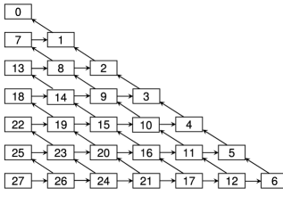
To conclude this section, we now use a simple example (n=6,m=2formulae-sequence𝑛6π‘š2n=6,m=2) to illustrate Algorithm 1. When m=2π‘š2m=2, each state has 333 parameters n0subscript𝑛0n_{0}, n1subscript𝑛1n_{1}, and n2subscript𝑛2n_{2}. Since n0+n1+n2=nsubscript𝑛0subscript𝑛1subscript𝑛2𝑛n_{0}+n_{1}+n_{2}=n, we could draw the state transition diagram as in Figure 1.
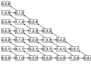
Refer to caption
Figure 1: State transition diagram for n=6,m=2formulae-sequence𝑛6π‘š2n=6,m=2. Self-loops are omitted. The nodes are labelled with the value of n0,n1,n2subscript𝑛0subscript𝑛1subscript𝑛2n_{0},n_{1},n_{2}.

Algorithm 1 computes E​[N2d​(n0,n1,n2)]𝐸delimited-[]superscriptsubscript𝑁2𝑑subscript𝑛0subscript𝑛1subscript𝑛2E[N_{2}^{d}(n_{0},n_{1},n_{2})] for each state (n0,n1,n2)subscript𝑛0subscript𝑛1subscript𝑛2(n_{0},n_{1},n_{2}) by the order shown in Figure 2. This is right because

  • β€’

    The expected number of runs from any state only depends on the number of runs from its descents in Figure 1.

  • β€’

    The computation of E​[N2d​(β‹―)]𝐸delimited-[]superscriptsubscript𝑁2𝑑⋯E[N_{2}^{d}(\cdots)] for any state is done after the computations for its descents by Figure 2.

Refer to caption
Figure 2: State transition diagram for n=6,m=2formulae-sequence𝑛6π‘š2n=6,m=2. The nodes are labelled by the computation order. The highest node, which represents (0,0,6)006(0,0,6) is labelled 0 because N2d​(0,0,6)superscriptsubscript𝑁2𝑑006N_{2}^{d}(0,0,6) is known to be 0.

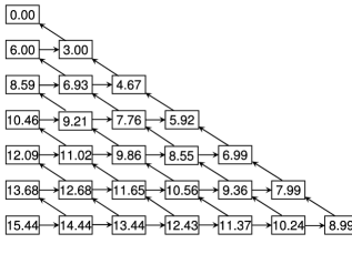
The values of E​[N2d​(n0,n1,n2)]𝐸delimited-[]superscriptsubscript𝑁2𝑑subscript𝑛0subscript𝑛1subscript𝑛2E[N_{2}^{d}(n_{0},n_{1},n_{2})] for each state (n0,n1,n2)subscript𝑛0subscript𝑛1subscript𝑛2(n_{0},n_{1},n_{2}) is shown in Figure 3.

Refer to caption
Figure 3: State transition diagram for n=6,m=2formulae-sequence𝑛6π‘š2n=6,m=2. The nodes are labelled by E​[N22​(n0,n1,n2)]𝐸delimited-[]superscriptsubscript𝑁22subscript𝑛0subscript𝑛1subscript𝑛2E[N_{2}^{2}(n_{0},n_{1},n_{2})].

7 Numerical Examples

We now engage in numerical exercises to support results in the last two sections, i.e. correctness of Algorithm 1 and the derived upper and lower bounds on E​(Dm,nd)𝐸superscriptsubscriptπ·π‘šπ‘›π‘‘E(D_{m,n}^{d}).

7.1 Algorithm

First, we give numerical results for the expected collection time when n=100𝑛100n=100 and m=1,2,3π‘š123m=1,2,3 respectively, in three tables. The results show that Algorithm 1 gives an expected delay consistent with the simulation results.

Table 1: m=1π‘š1m=1,n=100𝑛100n=100
d𝑑d 1 2 3 4 5
Algorithm 518.74 292.93 220.06 184.79 164.27
Simulation 518.69 292.40 219.33 184.59 164.18
Table 2: m=2π‘š2m=2,n=100𝑛100n=100
d𝑑d 1 2 3 4 5
Algorithm 728.81 418.69 327.02 286.75 264.84
Simulation 728.20 419.13 327.29 286.81 264.68
Table 3: m=3π‘š3m=3,n=100𝑛100n=100
d𝑑d 1 2 3 4 5
Algorithm 910.87 531.34 428.75 386.97 364.86
Simulation 910.09 531.33 428.72 386.65 364.90

7.2 Asymptotic Results

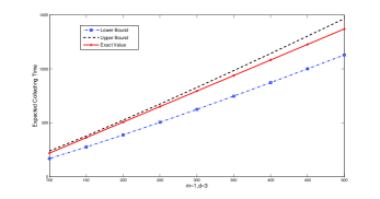
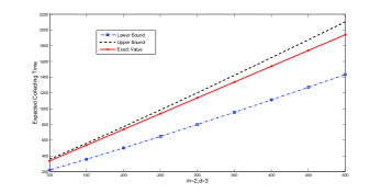
Two cases are considered: (d=3,m=1)formulae-sequence𝑑3π‘š1(d=3,m=1) and (d=3,m=2)formulae-sequence𝑑3π‘š2(d=3,m=2). For each case, three lines are plotted. First, the lower bound from Theorem 4.3 is plotted. Second, the upper bound is from Theorem 4.1 is computed. Finally, both plots are compared against the result computed from the algorithm for n𝑛n from 100100100 to 500500500. The results show that the upper bound and lower bound bound the expected collecting time very well. In fact, when mπ‘šm and d𝑑d are fixed, the upper bound and lower bound will both scale as 1d​E​(Dm,n1)1𝑑𝐸superscriptsubscriptπ·π‘šπ‘›1\frac{1}{d}E(D_{m,n}^{1}) as nβ†’βˆžβ†’π‘›n\rightarrow\infty.

Refer to caption
Figure 4: Asymptotics for m=1π‘š1m=1, d=3𝑑3d=3.
Refer to caption
Figure 5: Asymptotics for m=2π‘š2m=2, d=3𝑑3d=3.

8 Conclusion and Future Work

In this paper, we considered a generalized coupon collector problem where the coupon collector needs to collect mβ‰₯1π‘š1m\geq 1 sets of coupons and has the freedom of keeping one coupon out of dβ‰₯1𝑑1d\geq 1 coupons offered each time. We obtained asymptotically matching upper and lower bounds for the expected collection time. We also provided an algorithm to calculate the expected collection time exactly based on a state representation for the coupon collecting process. We should note that asymptotically even if the coupon collector is only allowed to keep 111 coupon out of the d𝑑d coupons, the needed time will still be shortened by a factor of d𝑑d, as if the coupon collector is allowed to keep all the d𝑑d coupons offered each time.

There is much avenue for future work on this problem. First, one could attempt to get a closed-form expression for E​(Dm,nd)𝐸superscriptsubscriptπ·π‘šπ‘›π‘‘E(D_{m,n}^{d}). Second, one could attempt to improve Algorithm 1. Algorithm 1 has a runtime of (n+mn)binomialπ‘›π‘šπ‘›{n+m\choose n}. To take advantage of this runtime requires constant time indexing. The direct approach is to index the states in an n𝑛n-dimensional matrix of size (n+1)m+1superscript𝑛1π‘š1(n+1)^{m}+1. However, since there are a total of (n+mn)binomialπ‘›π‘šπ‘›{n+m\choose n} states, a large fraction of the matrix space is not required. Hence, it would be helpful to find an algorithm which carries out triangular indexing in constant time. This would reduce the memory requirements and increase the range of parameters over which the problem is computationally feasible. One could further observe that although there are (n+mn)binomialπ‘›π‘šπ‘›{n+m\choose n} states, only (n+mβˆ’1mβˆ’1)binomialπ‘›π‘š1π‘š1{n+m-1\choose m-1} are actually needed at any time. So with constant time triangular indexing, one can reduce the memory requirements further although the gain from the second reduction is minimal.

Acknowledgment

The research is supported by NSF under CCF-0835706. The authors would like to thank the input of Wuhan Desmond Cai.

References

  • [1] Azar, Z., Broder, A., Karlin, A., and Upfal, E. (1999).Balanced Allocations. SIAM Journal on Computing, 29(1):180-200.
  • [2] Feller, W. (1950). An Introduction to Probability Theory. New York.
  • [3] Foata, D. and Zeilberger, D. (2003). The Collector’s Brotherhood Problem Using the Newman-Shepp Symbolic Method. Algebra Universalis, 49(4):387-395.
  • [4] Holst, L. (2001). Extreme Value Distributions for Random Coupon Collector and Birthday Problems. Extremes, 4:129-145.
  • [5] Kan, N. (2005). Margtingale Approach to the Coupon Collection Problem. Journal of Mathematical Siences, 127(1):1737-1744.
  • [6] Myers, A. and Wilf, H. (2003). Some New Aspects of the Coupon-Collector’s Problem. SIAM Journal on Discrete Mathematics, 17(1):1-17.
  • [7] Neal, P. (2008). The generalised coupon collector problem. Journal of Applied Probability, 45(3): 621-629.
  • [8] Newman, D. and Shepp, L. (1960). The Double Dixie Cup Problem. The American Mathamatical Monthly, 67(1):58-61.
  • [9] Sharif, M. and Hassibi, B. (2006). Delay Considerations for Opportunistic Scheduling in Broadcast Fading Channels. IEEE Transactions on Wireless Communication.