Abstract

Since the pioneering work of Gerhard Grüss dating back to 1935, Grüss’s inequality and, more generally, Grüss-type bounds for covariances have fascinated researchers and found numerous applications in areas such as economics, insurance, reliability, and, more generally, decision making under uncertainly. Grüss-type bounds for covariances have been established mainly under most general dependence structures, meaning no restrictions on the dependence structure between the two underlying random variables. Recent work in the area has revealed a potential for improving Grüss-type bounds, including the original Grüss’s bound, assuming dependence structures such as quadrant dependence (QD). In this paper we demonstrate that the relatively little explored notion of ‘quadrant dependence in expectation’ (QDE) is ideally suited in the context of bounding covariances, especially those that appear in the aforementioned areas of application. We explore this research avenue in detail, establish general Grüss-type bounds, and illustrate them with newly constructed examples of bivariate distributions, which are not QD but, nevertheless, are QDE. The examples rely on specially devised copulas. We supplement the examples with results concerning general copulas and their convex combinations. In the process of deriving Grüss-type bounds, we also establish new bounds for central moments, whose optimality is demonstrated.

Keywords and phrases: Grüss’s inequality, covariance bound, Hoeffding representation, Cuadras representation, quadrant dependence, quadrant dependence in expectation, copula, convex combination, Archimedean copula, Fréchet copula, Farlie-Gumbel-Morgenstern copula, central moments, Edmundson-Madansky bound.

1 Introduction

The covariance, say $\mathbf{Cov}[V,W]$ between two random variables $V$ and $W$, has played pivotal roles in numerous areas such as economics, finance, insurance, statistics, and, more generally, in decision making under uncertainty. For details on specific applications with references to many works in the areas that have greatly influenced our current research, we refer to Broll et al. [1], Egozcue et al. [9], [10], Furman and Zitikis [14], [15], [16], Zitikis [38]. A number of mathematics problems, especially those related to the theory of functions, have also been successfully tackled with the aid of covariance-type considerations (see, e.g., Dragomir and Agarwal [5], Dragomir and Diamond [6], Furman and Zitikis [12], [13], Izumino and Pečarić [25], Izumino et al. [26]). Solutions to problems in these areas often rely on determining the sign of covariances as well as on establishing their lower and upper bounds.

The random variables $V$ and $W$ are often unobservable but are known to be transformations (also called distortions) of some observable random variables $X$ and $Y$; that is, $V=\alpha(X)$ and $W=\beta(Y)$ for some functions $\alpha,\,\beta:\mathbf{R}\to\mathbf{R}$. Consequently, the covariance $\mathbf{Cov}[\alpha(X),\beta(Y)]$ becomes of interest. In a large number of applications, only one of the two random variables is distorted. In this paper we concentrate on this case, thus restricting ourselves to an in-depth analysis of the covariance

$$\mathbf{Cov}[X,\beta(Y)].$$ (1.1)

If compared to the more general covariance $\mathbf{Cov}[\alpha(X),\beta(Y)]$, this reduction of generality plays a significant role in providing us with additional technical tools, including the notion of ‘quadrant dependence in expectation’ (QDE) to be defined in Section 3 below, and thus in turn allows us to establish deeper results than those available in the literature under, say, the notion of quadrant dependence (QD). In applications where covariance (1.1) emerges, the distortion function $\beta$ might be, for example, a utility or value function (see, e.g., Broll et al. [1], Egozcue et al. [9], [10], and references therein), some insurance-premium loading function (see, e.g., Furman and Zitikis [14], [15], [16]; Sendov et al. [34], and references therein).

When estimating covariance (1.1), perhaps most naturally that comes first into our mind is the Cauchy-Schwarz inequality

$$\big{|}\mathbf{Cov}[X,\beta(Y)]\big{|}\leq\sqrt{\mathbf{Var}[X]}\,\sqrt{\mathbf{Var}[\beta(Y)]}\,,$$ (1.2)

where $\mathbf{Var}[X]$ is the variance (i.e., $\mathbf{Cov}[X,X]$) of the random variable $X$. Furthermore, assuming that there are finite intervals $[a,A]$ and $[b,B]$ such that $X\in[a,A]$ and $\beta(Y)\in[b,B]$ almost surely, from bound (1.2) we immediately obtain Grüss’s [23] inequality

$$\big{|}\mathbf{Cov}[X,\beta(Y)]\big{|}\leq{(A-a)(B-b)\over 4}$$ (1.3)

(see, e.g., Zitikis [38] for details and references). Inequalities (1.2) and (1.3) hold irrespectively of the dependence structure between $X$ and $\beta(Y)$, which implies that the inequalities also hold under the ‘worst possible’ dependence scenario, which is associated with the strongest dependence structure between $X$ and $\beta(Y)$, arising when $X=\beta(Y)$ almost surely. It is under this scenario that the optimality of the Grüss’s bound has been established in the literature, and we refer to, e.g., Dragomir [4], [7], Mitrinović et al. [31], Steele [35], and Zitikis [38] for further notes, examples, and references on the topic.

When the random variables $X$ and $\beta(Y)$ are independent, which in particular happens when the underlying random variables $X$ and $Y$ are such, then the covariance $\mathbf{Cov}[X,\beta(Y)]$ is zero. Hence, knowing how much and in what sense the random variables $X$ and $Y$ are dependent plays a significant role when investigating the magnitude of the covariance $\mathbf{Cov}[X,\beta(Y)]$ and its sign, among other properties. This line of research has been advocated by Zitikis [38] and Egozcue et al. [9], who have employed the notion of quadrant dependence to be defined rigorously in Section 3 below.

We conclude this section with a guide through the rest of this paper. In Section 2, we first show how the assumption of bivariate normality leads, via the well-known Stein’s Lemma, towards a Grüss-type covariance bound. We then extend this bivariate normal case into the formulation of a general Grüss-type covariance bound, which we aim at establishing in various situations throughout the current paper. In Section 3, we recall definitions of QD and QDE and their counterparts for copulas, and also relate these notions of dependence to Grüss-type covariance bounds. In Section 3 we also establish general results concerning convex mixtures of negative quadrant dependent (NQD) and positive quadrant dependent (PQD) copulas that provide a basis for constructing bivariate distributions which are QDE but not QD. We devote Section 4 to constructing several illustrative examples of copulas which are QDE but not QD; as far as we are aware of, these examples are the first ones in the literature. In Section 5, we establish QDE-based Grüss-type bounds for covariance (1.1), discuss their optimality and highlight the importance of having tight bounds for central moments of random variables. We investigate the latter bounds in great detail in Section 6. Since the QDE notion of dependence also naturally leads towards regression-based considerations, in Section 7 we establish regression-based Grüss-type bounds for covariance (1.1).

2 Formulation of the problem

Applications often suggest models for $(X,Y)$ but it may not be feasible to assume models for the pair $(X,\beta(Y))$ because the distortion function $\beta$ may change depending on, say, investor, insurer, etc. For this reason it is desirable to separate the underlying stochastic model, which is based on $(X,Y)$, from the class of distortion functions $\beta$.

Stein [36] noted that if the pair $(X,Y)$ follows the bivariate normal distribution and the function $\beta$ is differentiable, then

$$\mathbf{Cov}[X,\beta(Y)]=\mathbf{Cov}[X,Y]\mathbf{E}[\beta^{\prime}(Y)].$$ (2.1)

This equation, frequently known as Stein’s Lemma, separates the dependence structure from the distortion function $\beta$. For extensions and generalizations of this result, we refer to Furman and Zitikis [14], [15], [16], [17], and references therein. In particular, it has been observed that equation (2.1) is a direct consequence of the following one

$$\mathbf{Cov}[X,\beta(Y)]={\mathbf{Cov}[X,Y]\over\mathbf{Var}[Y]}\mathbf{Cov}[Y,\beta(Y)],$$ (2.2)

which separates the dependence structure of $(X,Y)$ from the distortion function $\beta$ but does not require the differentiability of $\beta$.

Now we rewrite equation (2.2) in the form

$$\mathbf{Cov}[X,\beta(Y)]=\mathbf{Corr}[X,Y]\,\mathbf{G}_{0}[X,Y,\beta],$$ (2.3)

which we call to be of the ‘Grüss form’ for reasons to be made clear below (Problem 2.1 below), where $\mathbf{Corr}[X,Y]$ is the Pearson correlation coefficient between $X$ and $Y$, and $\mathbf{G}_{0}[X,Y,\beta]$ is a ‘Grüss factor’ defined by

$$\mathbf{G}_{0}[X,Y,\beta]=\sqrt{{\mathbf{Var}[X]\over\mathbf{Var}[Y]}}\,\mathbf{Cov}[Y,\beta(Y)].$$

Note that the Grüss factor $\mathbf{G}_{0}[X,Y,\beta]$ does not depend on the bivariate distribution of $(X,Y)$ except that it depends on the cumulative distribution functions (cdf) $F$ and $G$ of the underlying random variables $X$ and $Y$, respectively, and also on the distortion function $\beta$. By the Cauchy-Schwarz inequality, $|\mathbf{G}_{0}[X,Y,\beta]|$ does not exceed the product of the standard deviations $\sqrt{\mathbf{Var}[X]}$ and $\sqrt{\mathbf{Var}[\beta(Y)]}$, which do not exceed $(A-a)/2$ and $(B-b)/2$, respectively, under what we call the ‘Grüss condition’:

• There are two finite intervals $[a,A]\subset\mathbf{R}$ and $[b,B]\subset\mathbf{R}$ such that $X\in[a,A]$ and $\beta(Y)\in[b,B]$ almost surely.

Hence, under the Grüss condition, we have that $\mathbf{G}_{0}[X,Y,\beta]$ does not exceed the right-hand side of bound (1.3), and we thus have that

$$\big{|}\mathbf{Cov}[X,\beta(Y)]\big{|}\leq\big{|}\mathbf{Corr}[X,Y]\big{|}\,{(A-a)(B-b)\over 4}.$$ (2.4)

Since $|\mathbf{Corr}[X,Y]|$ does not exceed $1$, bound (2.4) implies Grüss’s bound (1.3) irrespectively of the dependence structure between $X$ and $Y$. When these two random variables are independent, then the right-hand side of bound (1.3) is zero. This demonstrates the pivotal role of the dependence structure when sharpening Grüss’s bound.

Reflecting upon the notes above, we next put forward a general formulation of the problem that we shall tackle from various angles throughout this paper.

Problem 2.1

We are interested in establishing bounds of the form

$$\big{|}\mathbf{Cov}[X,\beta(Y)]\big{|}\leq\mathbf{D}[X,Y]\,\mathbf{G}[X,Y,\beta],$$ (2.5)

where

• $\mathbf{D}[X,Y]$ is a ‘dependence coefficient’, which must be equal to $0$ when the random variables $X$ and $Y$ are independent, and should not depend on the distortion function $\beta$;

• $\mathbf{G}[X,Y,\beta]$ is a ‘Grüss factor’, which should not depend on the dependence structure between $X$ and $Y$ but may depend on $\beta$ and the cdf’s $F$ and $G$ of $X$ and $Y$, respectively.

Throughout the paper we assume that the distortion function $\beta:\mathbf{R}\to\mathbf{R}$ is of bounded variation, meaning that it can be written as the difference $\beta=\beta_{1}-\beta_{2}$ of two non-decreasing functions $\beta_{1},\beta_{2}:\mathbf{R}\to\mathbf{R}$. The corresponding function $|\beta|:\mathbf{R}\to\mathbf{R}$ is defined by the equation $|\beta|(y)=\beta_{1}(y)+\beta_{2}(y)$. When $\beta$ is differentiable, then $d|\beta|(y)=|\beta^{\prime}(y)|dy$. Furthermore, we use $\mathbf{1}\{S\}$ for the indicator function of statement $S$ which is equal to $1$ when the statement $S$ is true and $0$ otherwise. Hence, in particular, for any random variable $Z$ and any real number $z$,

$$\tau_{z}(Z)=\mathbf{1}\{Z>z\}$$

is a random variable that takes on the value $1$ when $Z>z$ and $0$ otherwise. We shall frequently view $\tau_{z}(Z)$ as a random function of $z$. In our following considerations, we shall also use the sign-function, $\mathrm{sign}(x)$, which takes on three values: $-1$ when $x<0$, $0$ when $x=0$, and $+1$ when $x>0$.

3 QD and QDE random variables and copulas

One of the most fundamental equations that we utilize in the present paper is the Cuadras-Hoeffding representation

$$\mathbf{Cov}[\alpha(X),\beta(Y)]=\iint\mathbf{Cov}\big{[}\tau_{x}(X),\tau_{y}(Y)\big{]}d\alpha(x)\,d\beta(y)$$ (3.1)

of the covariance between the transformed random variables $\alpha(X)$ and $\beta(Y)$. The representation has been established by Cuadras [2] assuming, naturally and necessarily, that the expectations of $\alpha(X)$, $\beta(Y)$, and $\alpha(X)\beta(Y)$ are well-defined and finite. Covariance representation (3.1) generalizes the classical Hoeffding’s [24] representation established in the case $\alpha(x)=x$ and $\beta(x)=x$ (see also Sen [33]). The importance of representation (3.1) in our context is that it achieves a separation of the dependence structure present in $(X,Y)$ from the distortion functions $\alpha$ and $\beta$. Hence, in particular, the positive quadrant-dependence (definition follows) implies that $\mathbf{Cov}[X,Y]\geq 0$, and the negative quadrant-dependence implies that $\mathbf{Cov}[X,Y]\leq 0$. These are, of course, well-known facts (Lehmann [28]).

Definition 3.1 (Lehmann [28])

Two random variables $X$ and $Y$ are positively (resp. negatively) quadrant dependent if $\mathbf{Cov}\big{[}\tau_{x}(X),\tau_{y}(Y)\big{]}\geq 0$ (resp. $\leq 0$) for all $x,y\in\mathbf{R}$. We abbreviate this as PQD (resp. NQD), and when it is not important to specify whether the two random variables are PQD or NQD, then we simply say that they are quadrant dependent (QD).

As a special case of representation (3.1) we have the following one:

$$\mathbf{Cov}[X,\beta(Y)]=\iint\mathbf{Cov}\big{[}\tau_{x}(X),\tau_{y}(Y)\big{]}dx\,d\beta(y).$$ (3.2)

Note that the inner integral on the right-hand side of equation (3.2) is equal to $\mathbf{Cov}\big{[}X,\tau_{y}(Y)\big{]}$, and so representation (3.2) becomes

$$\mathbf{Cov}[X,\beta(Y)]=\int\mathbf{Cov}\big{[}X,\tau_{y}(Y)\big{]}d\beta(y).$$ (3.3)

The integrand on the right-hand side of equation (3.3) is related to the following definition.

Definition 3.2 (Kowalczyk and Pleszczynska [27])

A random variable $X$ is positively (resp. negatively) quadrant dependent in expectation on a random variable $Y$ if $\mathbf{Cov}\big{[}X,\tau_{y}(Y)\big{]}\geq 0$ (resp. $\leq 0$) for all $y\in\mathbf{R}$. We abbreviate this as $X$ is PQDE (resp. NQDE) on $Y$, and when it is not important to specify whether these two random variables are PQDE or NQDE, then we simply say that $X$ is quadrant dependent in expectation (QDE) on $Y$.

QDE is not a stronger notion than QD, which follows from the already noted but not explicitly written equation:

$$\mathbf{Cov}\big{[}X,\tau_{y}(Y)\big{]}=\int\mathbf{Cov}\big{[}\tau_{x}(X),\tau_{y}(Y)\big{]}dx.$$ (3.4)

For discussions and hints on potential applications of this notion of dependence, we refer to Kowalczyk and Pleszczynska [27], Wright [37], and references therein. One would actually expect that QDE is a weaker notion than QD, which means that there must be pairs $(X,Y)$ which are QDE (i.e., either NQDE or PQDE) but not QD (i.e, neither NQD nor PQD). Our search of the literature has not, however, revealed examples that would formally confirm this non-equivalence of QDE and QD. Hence, we next present general results pointing in the direction of non-equivalence, and we shall use them in Section 4 as our guide when constructing specific examples of bivariate distributions that are QDE but not QD.

The main tool that we are going to employ is the notion of copula, which is a surface $(u,v)\mapsto C(u,v)$ defined on the square $[0,1]\times[0,1]$ and such that $\mathbf{P}[X\leq x,Y\leq y]$ is equal to $C(F(x),G(y))$, where $F$ and $G$ are the cdf’s of $X$ and $Y$, respectively. Hence, in particular, we have the equation

$$\mathbf{Cov}\big{[}X,\tau_{y}(Y)\big{]}=\int\Big{(}C(F(x),G(y))-F(x)G(y)\Big{)}dx.$$ (3.5)

When the random variables $X$ and $Y$ have uniform (marginal) distributions, then we denote them by $U$ and $V$, respectively. In turn, we have the following reformulations of Definitions 3.1 and 3.2 in terms of the copula $C$, which is connected to the bivariate distribution of $(U,V)$ via the equation

$$\mathbf{P}[U\leq u,V\leq v]=C(u,v).$$

Namely, $U$ and $V$ are PQD (resp. NQD) if $C(u,v)\geq uv$ (resp. $C(u,v)\leq uv$) for all $u,v\in[0,1]$, and $U$ is PQDE (resp. NQDE) on $V$ if $\mathcal{C}(v)\geq 0$ (resp. $\mathcal{C}(v)\leq 0$) for all $v\in[0,1]$, where $\mathcal{C}(v)=\mathbf{Cov}\big{[}U,\tau_{v}(V)\big{]}$, that is (cf.  equation (3.5)),

$$\mathcal{C}(v)=\int_{0}^{1}\big{(}C(u,v)-uv\big{)}du.$$

In general, we have the following QD and QDE definitions for copulas.

Definition 3.3

Copula $(u,v)\mapsto C(u,v)$ is PQD (resp. NQD) if $C(u,v)\geq uv$ (resp. $C(u,v)\leq uv$) for all $u,v\in[0,1]$. The copula is QD if it is either NQD or PQD.

Definition 3.4

Copula $(u,v)\mapsto C(u,v)$ is PQDE (resp. NQDE) if $\mathcal{C}(v)\geq 0$ (resp. $\leq 0$) for all $v\in[0,1]$. The copula is QDE if it is either NQDE or PQDE.

Note 3.1

In Definition 3.4 it would be more precise to say that $U$ is PQDE (resp. NQDE) on $V$ if $\mathcal{C}(v)\geq 0$ (resp. $\leq 0$) for all $v\in[0,1]$. Analogously, $U$ is QDE on $V$ if $U$ is either NQDE or PQDE on $V$. We avoid this pedantry by always considering the ‘first variable’ to be (N/P)QDE on the ‘second variable’.

Hence, the problem that we are interested in at the moment is whether there are any copulas that are QDE (i.e., either NQDE or PQDE) but not QD (i.e, neither NQD nor PQD). The following two general theorems are fundamental in solving this problem, with illustrative examples provided in Section 4.

Theorem 3.1

Let $C_{0}(u,v)$ and $C_{1}(u,v)$ be NQD and PQD copulas, respectively. Denote their convex combination by $C_{\alpha}(u,v)=(1-\alpha)C_{0}(u,v)+\alpha C_{1}(u,v)$ with parameter $\alpha\in[0,1]$. Suppose that the surface

$$(u,v)\mapsto\frac{uv-C_{0}(u,v)}{C_{1}(u,v)-C_{0}(u,v)}$$ (3.6)

is not constant on $[0,1]\times[0,1]$. Then there exist $m,m^{\prime},M^{\prime},M\in[0,1]$ such that $0\leq m\leq m^{\prime}$, $M^{\prime}\leq M\leq 1$, and $m<M$, and such that the copula $C_{\alpha}$ is:

• NQD for $\alpha\in[0,m]$;

• neither NQD nor PQD for $\alpha\in(m,M)$;

• PQD for $\alpha\in[M,1]$;

• NQDE if and only if $\alpha\in[0,m^{\prime}]$ (it could be that $m=m^{\prime}$);

• neither NQDE nor PQDE for $\alpha\in(m^{\prime},M^{\prime})$ (it could be that $m^{\prime}\geq M^{\prime}$, in which case the interval $(m^{\prime},M^{\prime})$ is empty);

• PQDE if and only if $\alpha\in[M^{\prime},1]$ (it could be that $M=M^{\prime}$).

Proof. Let $I_{-}=\{\alpha\in[0,1]\,:\,C_{\alpha}\hbox{ is NQD}\}$ and $I_{+}=\{\alpha\in[0,1]\,:\,C_{\alpha}\hbox{ is PQD}\}$. We have the following facts:

1. $0\in I_{-}$ and $1\in I_{+}$.

2. $I_{-}$ (similarly $I_{+}$) is a closed subspace of $[0,1]$. Namely, if $C_{\alpha_{k}}(u,v)-uv\leq 0$ for all $u,v\in[0,1]$ and $\alpha_{k}\to\alpha$, then $C_{\alpha}(u,v)-uv\leq 0$ for all $u,v\in[0,1]$.

3. $I_{-}$ (similarly $I_{+}$) is a connected space. Namely, if $\alpha,\beta\in I_{-}$, then $C_{\gamma}$ for any $\gamma\in[\alpha,\beta]$ is a convex combination of $C_{\alpha}$ and $C_{\beta}$, and so it is NQD.

4. $I_{-}$ and $I_{+}$ are closed intervals (it follows from 2 and 3).

5. $I_{-}\cap I_{+}=\emptyset$. We prove this by contradiction. Suppose that there exists $\alpha\in I_{-}\cap I_{+}$. Then $C_{\alpha}$ is NQD and PQD. This implies that $(1-\alpha)C_{0}(u,v)+\alpha C_{1}(u,v)-uv=0$ for all $u,v\in[0,1]$. Hence, function (3.6) is equal to the constant $\alpha$; a contradiction.

In view of the above facts we have that $I_{-}=[0,m]$ and $I_{+}=[M,1]$ with $m<M$, and the first three statements of Theorem 3.1 follow. In a similar way, but working with the function

$$\mathcal{C}_{\alpha}(v)=\int_{0}^{1}\big{(}C_{\alpha}(u,v)-uv\big{)}du,$$ (3.7)

we establish the other three statements of Theorem 3.1. Note that NQD (PQD) implies NQDE (PQDE), and so we must have $m\leq m^{\prime}$ and $M^{\prime}\leq M$. This completes the proof of Theorem 3.1.   

Note 3.2

If we have $m<m^{\prime}$, then there are $\alpha$ values such that the copula $C_{\alpha}$ is neither NQD nor PQD, but it is NQDE. Similarly, if we have $M^{\prime}<M$, then there are $\alpha$ values such that the copula $C_{\alpha}$ is neither NQD nor PQD, but it is PQDE.

Theorem 3.2

Let the assumptions of Theorem 3.1 be satisfied, and let $\mathcal{C}_{\alpha}(v)$ be given by equation (3.7). Furthermore, assume that there is a constant $\kappa\in[0,1]$ such that

$$\frac{\mathcal{C}_{0}(v)}{\mathcal{C}_{0}(v)-\mathcal{C}_{1}(v)}=\kappa$$

for all $v\in(0,1)$. Then there is an open interval of $\alpha$ values such that the copula $C_{\alpha}$ is neither NQD nor PQD, but it is either NQDE or PQDE.

Proof. We have that $\mathcal{C}_{\kappa}(v)=0$ for all $v\in[0,1]$. Thus, the copula $C_{\kappa}$ is both PQDE and NQDE. By the previous theorem, we have that $M^{\prime}\leq\kappa\leq m^{\prime}$. Since $m\leq m^{\prime}$, $M^{\prime}\leq M$ and $m<M$, we deduce that $m<m^{\prime}$ or $M^{\prime}<M$. Consider these two cases separately: 1) if $m<m^{\prime}$, then for any $\alpha\in(m,m^{\prime}]$ the copula $C_{\alpha}$ is neither NQD nor PQD, but it is NQDE, and 2) if $M^{\prime}<M$, then for any $\alpha\in[M^{\prime},M)$ the copula $C_{\alpha}$ is neither NQD nor PQD, but it is PQDE. This completes the proof of Theorem 3.2.   

4 Examples of QDE copulas which are not QD

Here we give three examples of QDE copulas that are not QD. In the first two examples we choose NQD and PQD copulas such that their convex combinations are not QD but, nevertheless, are QDE. The third example is based on a copula which is not QD but, under an appropriate choice of marginal distributions, produces a bivariate distribution that is not QD but, nevertheless, is QDE. These three examples open up broad avenues for constructing QDE copulas that are not QD, using a myriad of existing copulas whose QD-type properties have been documented in the literature (e.g., Nelsen [32]). For discussions concerning copulas in the context of actuarial, financial, and other applications, we refer to, for example, Denuit et al. [3], Genest and Favre [18], Genest et al. [19], McNeil et al. [29], and references therein.

Example 4.1

The Fréchet lower-bound (FL) copula

$$C_{FL}(u,v)=\max\{0,u+v-1\}$$

is NQD, and the Fréchet upper-bound (FU) copula

$$C_{FU}(u,v)=\min\{u,v\}$$

is PQD. Both are defined on the unit square $[0,1]\times[0,1]$. Let $C_{\alpha}$ be the convex combination of the two Fréchet copulas (cf. McNeil et al. [29]):

$$C_{\alpha}(u,v)=(1-\alpha)C_{FL}(u,v)+\alpha C_{FU}(u,v),$$ (4.1)

where $\alpha\in(0,1)$. We see from Figure 4.1

Figure 4.1: The surface $(u,v)\mapsto\mathrm{sign}[C_{\alpha}(u,v)-uv]$ when $\alpha=1/4$ (left top panel), $\alpha=1/2$ (center top panel), and $\alpha=3/4$ (right top panel) with the corresponding contour plots beneath them.

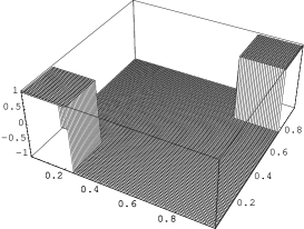
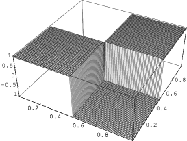
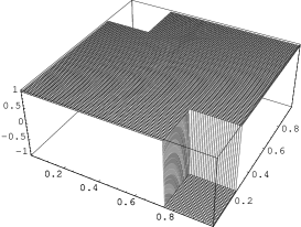
that the copula $C_{\alpha}$ is neither PQD nor NQD. To check whether $C_{\alpha}$ is QDE (i.e., either PQDE or NQDE), we calculate the integral

$$\mathcal{C}_{\alpha}(v)=\int_{0}^{1}\big{(}C_{\alpha}(u,v)-uv\big{)}du=v(1-v)\bigg{(}\alpha-{1\over 2}\bigg{)}.$$ (4.2)

Hence, $\mathcal{C}_{\alpha}(v)\leq 0$ for all $v\in[0,1]$ if and only if $\alpha\leq 1/2$, meaning that the copula $C_{\alpha}$ is NQDE. Likewise, $\mathcal{C}_{\alpha}(v)\geq 0$ for all $v\in[0,1]$ if and only if $\alpha\geq 1/2$, meaning that $C_{\alpha}$ is PQDE. Hence, for example, when $\alpha=1/4$, then $C_{\alpha}$ is neither PQD nor NQD but it is NQDE. Likewise, when $\alpha=3/4$, then $C_{\alpha}$ is neither PQD nor NQD but it is PQDE. This concludes Example 4.1.

Example 4.2

Here we first choose the Farlie-Gumbel-Morgenstern (FGM) copula

$$C_{FGM}(u,v)=uv\big{(}1+\theta(1-u)(1-v)\big{)}$$

with $\theta\in[-1,1]$; we set the parameter $\theta$ to $-1$ throughout this example to make the FGM copula NQD. Next we choose the already noted Fréchet upper-bound copula $C_{FU}(u,v)=\min\{u,v\}$, which is PQD. Let $\alpha\in(0,1)$ be a parameter, and let $C_{\alpha}$ be the convex combination of the above two copulas:

$$C_{\alpha}(u,v)=(1-\alpha)C_{FGM}(u,v)+\alpha C_{FU}(u,v).$$ (4.3)

We have that

$$C_{\alpha}(u,v)-uv =\alpha\big{(}\min\{u,p\}-uv\big{)}-(1-\alpha)uv(1-u)(1-v)$$

$$=\left\{\begin{array}[]{ll}u(1-v)\big{(}1-(1-\alpha)(1+v(1-u))\big{)}&\hbox{when }\,u\leq v,\\ v(1-u)\big{(}1-(1-\alpha)(1+u(1-v))\big{)}&\hbox{when }\,u\geq v.\end{array}\right.$$ (4.6)

Hence, $C_{\alpha}(u,v)-uv\geq 0$ for only those $(u,v)\in[0,1]\times[0,1]$ that are between (cf.  equation (4.6)) the zero-curve

$$U_{\alpha}=\big{\{}(u,v):\,(1-\alpha)(1+v(1-u))=1\big{\}}\quad\bigg{[}\textrm{ that is, }v=v_{U}(u)={1\over 1-u}\,{\alpha\over 1-\alpha}\bigg{]}$$

from above, and the zero-curve

$$L_{\alpha}=\big{\{}(u,v):\,(1-\alpha)(1+u(1-v))=1\big{\}}\quad\bigg{[}\textrm{ that is, }v=v_{L}(u)=1-{1\over u}\,{\alpha\over 1-\alpha}\bigg{]}$$

from below. We illustrate the two curves in Figure 4.2.

Figure 4.2: The surface $(u,v)\mapsto\mathrm{sign}[C_{\alpha}(u,v)-uv]$ when $\alpha=1/6$ (left top panel), $\alpha=1/5$ (center top panel), and $\alpha=1/4$ (right top panel) with the zero-curves $U_{\alpha}$ and $L_{\alpha}$ in the corresponding plots beneath them.

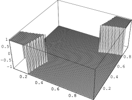
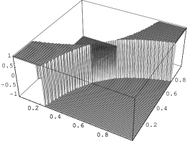
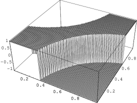
Note that the curves intersect in the interior of the square $[0,1]\times[0,1]$ only when $\alpha\in(0,1/5)$ and touch each other at one point when $\alpha=1/5$. As to the PQDE or NQDE, we calculate the integral

$$\mathcal{C}_{\alpha}(v)=\int_{0}^{1}\big{(}C_{\alpha}(u,v)-uv\big{)}du={v(1-v)\over 2}\bigg{(}{4\over 3}\,\alpha-{1\over 3}\bigg{)}.$$ (4.7)

Hence, $\mathcal{C}_{\alpha}(v)\leq 0$ for all $v\in(0,1)$ meaning that $C_{\alpha}$ is NQDE if and only if $\alpha\leq 1/4$, and $\mathcal{C}_{\alpha}(v)\geq 0$ for all $v\in(0,1)$ meaning that $C_{\alpha}$ is PQDE if and only if $\alpha\geq 1/4$. This concludes Example 4.2.

Example 4.3

We model the pair $(X,Y)$ using the following Archimedean copula (Genest and MacKay [21], [22]; Genest and Ghoudi [20]; see also Nelsen [32] for additional information and references)

$$C_{\alpha}(u,v)=\max\left\{0,1-\left((1-u^{\alpha})^{1/\alpha}+(1-v^{\alpha})^{1/\alpha}\right)^{\alpha}\right\}^{1/\alpha},$$

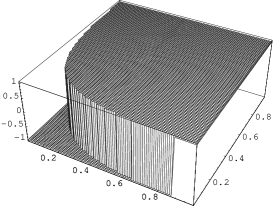
where $\alpha\in(0,1)$ is parameter. The copula $C_{\alpha}(u,v)$ is not QD. The zero-curve $Z_{\alpha}(u,v)=C_{\alpha}(u,v)-uv=0$, which separates the NQD region from the PQD region, is given by

$$Z_{\alpha}=\big{\{}(u,v):\,(1-u^{\alpha})^{1/\alpha}+(1-v^{\alpha})^{1/\alpha}=(1-u^{\alpha}v^{\alpha})^{1/\alpha}\big{\}},$$

depicted in Figure 4.3.

Figure 4.3: The surface $(u,v)\mapsto\mathrm{sign}[C_{\alpha}(u,v)-uv]$ when $\alpha=5/10$ (left top panel), $\alpha=7/10$ (center top panel), and $\alpha=9/10$ (right top panel) with the zero-curve $Z_{\alpha}$ in the corresponding plots beneath them.

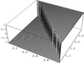
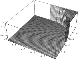
Concerning the QDE property, we want to know if and when the function $\mathcal{C}_{\alpha}$ defined by the formula

$$\mathcal{C}_{\alpha}(v)=\int_{0}^{1}\big{(}C_{\alpha}(u,v)-uv\big{)}du$$

is positive or negative. Our experimental analysis has revealed that this function is negative for some $v\in[0,1]$ and positive for other $v$, and this applies to every $\alpha\in(0,)]$. For an illustration, we have produced Figure 4.4.

Figure 4.4: The function $v\mapsto\mathcal{C}_{\alpha}(v)$ when $\alpha=5/10$ (left panel), $\alpha=7/10$ (center panel), and $\alpha=9/10$ (right panel). In every case, there are regions (not necessarily clearly visible in the graphs) where the function is strictly positive and strictly negative.

This implies that for the purpose of constructing QDE pairs of random variables we cannot choose both marginal cdf’s uniform. Hence, we choose only the first marginal cdf (i.e., that of $X$) uniform. Since the second marginal cdf (i.e., that of $Y$) cannot be uniform, nor any other continuous cdf, we construct a discrete cdf $G$ or, equivalently, a discrete random variable $Y$ in such a way that $U(=X)$ is PQDE on $Y$.

First we note that, for every $v\in(0,1)$,

• $C_{\alpha}(u,v)-uv$ is positive for some $u\in(0,1)$ and negative for some other $u\in(0,1)$, thus violating the QD property.

To verify this non-QD property rigorously, we first rewrite the copula $C_{\alpha}(u,v)$ as $\max\{0,P(u,v)\}^{1/{\alpha}}$ with the notation

$$P(u,v)=1-((1-u^{\alpha})^{1/{\alpha}}+(1-v^{\alpha})^{1/{\alpha}})^{\alpha}.$$

For every fixed $v$ and when $u=0$, then we have $P(0,v)=1-(1+(1-v^{\alpha})^{1/{\alpha}})^{\alpha}<0$. Thus, $C_{\alpha}(u,v)=0$ in a neighbourhood of $u=0$. From this we deduce that $C_{\alpha}(u,v)-uv<0$ when $u\in(0,\epsilon)$ for some $\epsilon>0$. In a neighbourhood of $u=1$, we have that $C_{\alpha}(u,v)-uv$ is equal to $P(u,v)^{1/{\alpha}}-uv$, which is a differentiable function. The partial derivative $(d/du)(P(u,v)^{1/{\alpha}}-uv)$ at the point $u=1$ is negative. Hence, the function $u\mapsto P(u,v)^{1/{\alpha}}-uv$ is decreasing in a neghbourhood of $1$. When $u=1$, then we have $P(1,v)^{1/{\alpha}}=v$ and thus $P(1,v)^{1/{\alpha}}-1\cdot v=0$. Hence, the function $u\mapsto P(u,v)^{1/{\alpha}}-uv$ or, equivalently, $u\mapsto C_{\alpha}(u,v)-uv$ is positive in a neighbourhood to the left of $u=1$. This establishes the property formulated under the bullet above.

Next, in view of the equation

$$\mathbf{Cov}\big{[}U,\tau_{y}(Y)\big{]}=\mathcal{C}_{\alpha}(G(y)),$$ (4.8)

we construct $Y$ such that its support is in an interval $[v^{*},v^{**}]\subseteq(0,1)$ and

• for every $v\in[v^{*},v^{**}]$, we have $\mathcal{C}_{\alpha}(v)>0$, thus assuring that the PQDE property holds, provided that $Y$ takes only on values in the interval $[v^{*},v^{**}]$.

The construction of the aforementioned $Y$ is as follows. We choose a set of $K$ points $v_{k}>v^{*}$ such that $\sum_{k=1}^{K-1}v_{k}<v^{**}$ and $\sum_{k=1}^{K}v_{k}=1$. Define the cdf $G$ by the formula

$$G(y)=\sum_{k=1}^{K}v_{k}\mathbf{1}\{y_{k}\leq y\},$$

where $y_{1}<y_{2}<\cdots<y_{K}$ are real numbers. In other words, the random variable $Y$ takes on the values $y_{k}$ with the probabilities $v_{k}$. Note that the range of the cdf $G$ is the set $\{0,v_{1},v_{1}+v_{2},\dots,\sum_{k=1}^{K-1}v_{k},1\}$. By construction, $\mathcal{C}_{\alpha}(v)>0$ for all $v\in\{v_{1},v_{1}+v_{2},\dots,\sum_{k=1}^{K-1}v_{k}\}$. Hence, in order to verify that $\mathcal{C}_{\alpha}(G(Y))\geq 0$ for all real $y\in\mathbf{R}$, we are only left to check that $\mathcal{C}_{\alpha}(v)\geq 0$ for $v\in\{0,1\}$, but this holds because $C_{\alpha}(u,0)=0$ and $C_{\alpha}(u,1)=u$.

In summary, we have constructed a pair $(U,Y)$ such that $\mathbf{Cov}\big{[}U,\tau_{y}(Y)\big{]}\geq 0$ for all $y\in\mathbf{R}$, that is, $U(=X)$ is PQDE on $Y$, but the pair is not QD, that is, it is neither PQD nor NQD. This concludes Example 4.3.

5 QDE-based Grüss-type covariance bounds

From the previous two sections we know that the set of QDE random pairs is larger than the set of QD pairs. In this sense, establishing Grüss-type covariance bounds under the QDE assumption would be an extension of those established under the QD assumption. We explore such QDE-based results in the current section. In what follows, we use the notation

$$\mathbf{A}_{k}[Z]=\big{(}\mathbf{E}\big{[}|Z-\mathbf{E}[Z]|^{k}\big{]}\big{)}^{1/k}.$$

The next theorem, whose proof is a consequence of equation (3.3), utilizes the QDE notion and establishes a sharper bound than Grüss’s original bound (1.3).

Theorem 5.1

For every pair $p,q\in(1,\infty)$ such that $p^{-1}+q^{-1}=1$, we have the bound

$$\big{|}\mathbf{Cov}[X,\beta(Y)]\big{|}\leq\mathbf{D}_{p}[X,Y]\,\mathbf{G}_{p}[X,Y,\beta],$$ (5.1)

where the QDE-based dependence coefficient is

$$\mathbf{D}_{p}[X,Y]=\sup_{y}{\big{|}\mathbf{Cov}\big{[}X,\tau_{y}(Y)\big{]}\big{|}\over\mathbf{A}_{p}[X]\mathbf{A}_{q}[\tau_{y}(Y)]}$$

with the supremum taken over all $y\in\mathbf{R}$ such that $G(y)\in(0,1)$, that is, over the support of the random variable $Y$, and where the QDE-based Grüss factor is

$$\mathbf{G}_{p}[X,Y,\beta]=\mathbf{A}_{p}[X]\int\mathbf{A}_{q}[\tau_{y}(Y)]\,d|\beta|(y).$$

Before discussing properties of the QDE-based dependence coefficient and Grüss’s factor, we first show that bound (5.1) implies Grüss’s bound (1.3).

Statement 5.1

Setting $p=2$ and $\beta(x)=\beta_{0}(x)\equiv x$, we have that under the Grüss conditions on $X$ and $Y$, Grüss’s bound (1.3) follows from Theorem 5.1.

Proof. Since $\mathbf{D}_{2}[X,Y]\leq 1$, we only need to show that

$$\mathbf{G}_{2}[X,Y,\beta_{0}]\leq{(A-a)(B-b)\over 4}.$$ (5.2)

Since $G(y)(1-G(y))$ does not exceed $1/4$ and is equal to $0$ outside the support of $Y$, and since $Y\in[b,B]\subset\mathbf{R}$ almost surely, we have that $\mathbf{G}_{2}[X,Y,\beta_{0}]$ does not exceed $\sqrt{\mathbf{Var}[X]}\,(B-b)/2$. Furthermore, since $X\in[a,A]\subset\mathbf{R}$ almost surely, then (see, e.g., Zitikis [38], p. 16) $\sqrt{\mathbf{Var}[X]}$ does not exceed $(A-a)/2$. Hence, bound (5.2) holds.   

The dependence coefficient $\mathbf{D}_{p}[X,Y]$ is always in the interval $[0,1]$. It takes on the value $0$ when $X$ and $Y$ are independent. Furthermore, the coefficient achieves its upper bound $1$, as seen from the following statement.

Statement 5.2

The dependence coefficient $\mathbf{D}_{p}[X,Y]$ achieves its upper bound $1$.

Proof. Given $Y$, let $X$ be the random variable $X_{0}$ defined by the equation

$$X_{0}=\varepsilon\big{|}\tau_{y_{0}}(Y)-\mathbf{E}[\tau_{y_{0}}(Y)]\big{|}^{q/p}\mathrm{sign}\big{(}\tau_{y_{0}}(Y)-\mathbf{E}[\tau_{y_{0}}(Y)]\big{)},$$

where

• the number $y_{0}>0$ is any but fixed, and

• the random variable $\varepsilon$, independent of $Y$, takes on the two values $\pm 1$ with same probabilities $p=1/2$.

The expectation $\mathbf{E}[X_{0}]$ is equal to $0$. The absolute value $|X_{0}|$ is equal to $\big{|}\tau_{y_{0}}(Y)-\mathbf{E}[\tau_{y_{0}}(Y)]\big{|}^{q/p}$. The covariance $\mathbf{Cov}[X_{0},\tau_{y}(Y)]$ is equal to $\mathbf{A}_{q}^{q}[\tau_{y}(Y)]$. Hence, $\mathbf{D}_{p}[X_{0},Y]=1$.   

The magnitude of the coefficient $\mathbf{D}_{p}[X,Y]$ depends on the dependence structure between $X$ and $Y$, as well as on the marginal cdf’s of the two random variables. For example, in the case of independent $X$ and $Y$, we have $\mathbf{D}_{p}[X,Y]=0$. Less trivial and thus more interesting examples follow.

Example 5.1

Consider the convex combination of the lower and upper Fréchet copulas as defined by equation (4.1). Both $X=U$ and $Y=V$ have uniform distributions on the interval $[0,1]$, and thus

$$\mathbf{A}_{p}[U]={1\over 2(p+1)^{1/p}}\quad\textrm{and}\quad\mathbf{A}_{q}[\tau_{v}(V)]=\kappa_{q}^{1/q}(v),$$ (5.3)

where the function $\kappa_{q}:[0,1]\to[0,1/2]$ is defined by

$$\kappa_{q}(v)=v(1-v)^{q}+(1-v)v^{q}.$$

Furthermore, since $\mathbf{Cov}\big{[}U,\tau_{v}(V)\big{]}=\mathcal{C}_{\alpha}(v)$ with $\mathcal{C}_{\alpha}(v)$ given by equation (4.2), we have that

$$\mathbf{D}_{p}[U,V]=2(p+1)^{1/p}\bigg{|}\alpha-{1\over 2}\bigg{|}\sup_{0<v<1}{v(1-v)\over\kappa_{q}^{1/q}(v)}.$$ (5.4)

Recall that $q=p/(p-1)$. The QDE-based Grüss factor is

$$\mathbf{G}_{p}[U,V,\beta]={1\over 2(p+1)^{1/p}}\int_{0}^{1}\kappa_{q}^{1/q}(v)d|\beta|(v).$$ (5.5)

In the special case when $p=2$ and $\beta(v)=\beta_{0}(v)\equiv v$, we have that

$$\mathbf{D}_{2}[U,V] =\sqrt{3}\,\bigg{|}\alpha-{1\over 2}\bigg{|},$$ (5.6)

$$\mathbf{G}_{2}[U,V,\beta_{0}] ={1\over 2\sqrt{3}}\int_{0}^{1}\sqrt{v(1-v)}\,dv={\pi\over 16\sqrt{3}}.$$ (5.7)

Bound (5.1) therefore implies that

$$\big{|}\mathbf{Cov}[X,Y]\big{|}\leq{\pi\over 16}\,\bigg{|}\alpha-{1\over 2}\bigg{|}\approx 0.19635\,\bigg{|}\alpha-{1\over 2}\bigg{|},$$ (5.8)

whereas the exact calculation using, for example, the equation $\mathbf{Cov}[X,Y]=\int_{0}^{1}\mathcal{C}_{\alpha}(v)dv$ and formula (4.2) gives the value

$$\mathbf{Cov}[X,Y]={1\over 6}\,\bigg{(}\alpha-{1\over 2}\bigg{)}\approx 0.166667\,\bigg{(}\alpha-{1\over 2}\bigg{)}.$$ (5.9)

This concludes Example 5.1.

Example 5.2

Consider the convex combination of the Farlie-Gumbel-Morgenstern and upper-Fréchet copulas as defined by equation (4.3). Just like in the previous example, both $X=U$ and $Y=V$ have uniform distributions on the interval $[0,1]$. Thus, equations (5.3) hold in the current case as well. The covariance $\mathbf{Cov}\big{[}U,\tau_{v}(V)\big{]}$ is, however, different: it is equal to $\mathcal{C}_{\alpha}(v)$ given by equation (4.7). Hence, the QDE-based dependence coefficient is

$$\mathbf{D}_{p}[U,V]=(p+1)^{1/p}\bigg{|}{4\over 3}\,\alpha-{1\over 3}\bigg{|}\sup_{0<v<1}{v(1-v)\over\kappa_{q}^{1/q}(v)}.$$ (5.10)

Recall that $q=p/(p-1)$. Note that the QDE-based Grüss factor $\mathbf{G}_{p}[U,V,\beta]$ is unaffected by the change of the dependence structure and therefore has the same expression as in previous Example 5.1 (see eq. (5.5)). In the special case when $p=2$, from the above formulas we have that

$$\mathbf{D}_{2}[U,V]={\sqrt{3}\over 2}\,\bigg{|}{4\over 3}\,\alpha-{1\over 3}\bigg{|}.$$ (5.11)

Bound (5.1) therefore implies that

$$\big{|}\mathbf{Cov}[X,Y]\big{|}\leq{\pi\over 32}\,\bigg{|}{4\over 3}\,\alpha-{1\over 3}\bigg{|}\approx 0.0981748\,\bigg{|}{4\over 3}\,\alpha-{1\over 3}\bigg{|},$$ (5.12)

whereas the exact calculation using the equation $\mathbf{Cov}[X,Y]=\int_{0}^{1}\mathcal{C}_{\alpha}(v)dv$ and formula (4.7) gives the value

$$\mathbf{Cov}[X,Y]={1\over 12}\,\bigg{(}{4\over 3}\,\alpha-{1\over 3}\bigg{)}\approx 0.0833333\,\bigg{(}{4\over 3}\,\alpha-{1\over 3}\bigg{)}.$$ (5.13)

This concludes Example 5.2.

6 Estimating the QDE-based Grüss factor

In Example 5.1 we calculated the QDE-based Grüss factor $\mathbf{G}_{p}[U,V,\beta]$ in the case of uniform random variables $U$ and $V$. In Statement 5.1 we estimated $\mathbf{G}_{2}[X,Y,\beta_{0}]$ under the Grüss condition on $X$ and $Y$. In the current section we develop general results that aid in establishing tight upper bounds for the QDE-based (general) Grüss factor $\mathbf{G}_{p}[X,Y,\beta]$. Specifically, upon expressing the quantities $\mathbf{A}_{p}[X]$ and $\mathbf{A}_{q}[\tau_{y}(Y)]$ by the formulas

$$\mathbf{A}_{p}[X]=\big{(}\mathbf{E}\big{[}|X-\mu|^{p}\big{]}\big{)}^{1/p}$$

and

$$\mathbf{A}_{q}[\tau_{y}(Y)]=\kappa_{q}^{1/q}(G(y)),$$

where the mean $\mu=\mathbf{E}[X]$, the cdf $G$ of $Y$, and the function

$$\kappa_{q}(x)=x(1-x)^{q}+(1-x)x^{q},$$

we see that estimating $\mathbf{G}_{p}[X,Y,\beta]$ relies on tight bounds for the $p^{\textrm{th}}$ central moment $\mathbf{E}\big{[}|X-\mu|^{p}\big{]}$ as well as on the function $\kappa_{q}(x)$. Interestingly, as we shall see from Theorem 6.1 below, which is the main result of this section, tight upper bounds for the $p^{\textrm{th}}$ central moment also crucially rely on the function $\kappa_{p}(x)$.

Theorem 6.1

Let $X$ be a random variable with support in $[a,A]$. Then, for every $p\geq 1$, we have that

$$\mathbf{E}\big{[}|X-\mu|^{p}\big{]}\leq(A-a)^{p}\kappa_{p}\bigg{(}\frac{\mu-a}{A-a}\bigg{)}.$$ (6.1)

Consequently, with the notation $K_{p}=\sup_{x\in[0,1]}\kappa_{p}(x)$, we have that

$$\mathbf{E}\big{[}|X-\mu|^{p}\big{]}\leq(A-a)^{p}K_{p}.$$ (6.2)

Furthermore, when $p\to\infty$, we have that

$$(1+p)K_{p}\to e^{-1}.$$ (6.3)

The maximum $K_{p}$ of the function $\kappa_{p}(x)$ is achieved at a unique point $x=x_{p}$ in the interval $[1/(1+p),1/2]$ and thus, by symmetry, also at the point $1-x_{p}$ in the interval $[1/2,p/(1+p)]$. The point $x_{p}$ is such that, when $p\to\infty$,

$$(1+p)x_{p}\to 1.$$ (6.4)

Note 6.1

Bound (6.1) is sharp in the sense that there is a random variable $X=X_{1}$ for which the inequality turns into an equality. Namely, let $X_{1}$ take on only two values, $a$ and $A$, with the probabilities $\mathbf{P}[X_{1}=a]=(A-\mu)/(A-a)$ and $\mathbf{P}[X_{1}=A]=(\mu-a)/(A-a)$, respectively. Inequality (6.11) becomes an equality.

Note 6.2

When $p=2$, then $K_{p}=1/4$, which plays a crucial role in deriving the Grüss bound. Formulas for $K_{p}$ for the integers $1\leq p\leq 6$ are given in Table 6.1

$$\begin{array}[]{|r|r|r|}\hline\cr{p}&{x_{p}}&{K_{p}}\\ \hline\cr{1}&{\frac{1}{2}}={0.50000000000000000000}&{\frac{1}{2}}={0.500000000000000000000}\\ \hline\cr{2}&{\frac{1}{2}}={0.50000000000000000000}&{\frac{1}{4}}={0.250000000000000000000}\\ \hline\cr{3}&{\frac{1}{2}}={0.50000000000000000000}&{\frac{1}{8}}={0.125000000000000000000}\\ \hline\cr{4}&{\frac{3-\sqrt{3}}{6}}={0.21132486540518711775}&{\frac{1}{12}}={0.083333333333333333333}\\ \hline\cr{5}&{\frac{3-\sqrt{6\sqrt{10}-15}}{6}}={0.16776573020222127904}&{\frac{5\sqrt{10}-14}{27}}={0.067088455586736913333}\\ \hline\cr{6}&{\frac{15-\sqrt{60\sqrt{10}-75}}{30}}={0.14294933504534875025}&{\frac{4\sqrt{10}-5}{135}}={0.056660078819803832059}\\ \hline\cr{7}&{0.12500637707104845945}&{0.049087405277751670707}\\ \hline\cr{8}&{0.11111148199402853664}&{0.043304947663997051030}\\ \hline\cr{9}&{0.10000001858448876931}&{0.038742049800000743380}\\ \hline\cr{10}&{0.09090909172727279935}&{0.035049389983188641270}\\ \hline\cr\end{array}$$

Table 6.1: The values of $x_{p}$ and $K_{p}$ for the integers $1\leq p\leq 10$.

along with the corresponding values of $x_{p}\in[0,1/2]$. By symmetry, the maximum $K_{p}$ is also achieved at the point $1-x_{p}\in[1/2,1]$. However, throughout this paper we use $x_{p}$ to denote the only existing point in the interval $[0,1/2]$ such that

$$K_{p}=\kappa_{p}(x_{p}).$$

(We refer to the proof of Theorem 6.1 for the existence and uniqueness of $x_{p}$.) When $p$ becomes large, expressions for $x_{p}$ and $K_{p}$ become unwieldy, due to the fact that $x_{p}$ is a certain solution to a polynomial equation of a high degree, for which explicit solutions are not known to the best of our knowledge. For this reason, in Table 6.1 we have provided only numerical values of $x_{p}$ and $K_{p}$ for the integers $7\leq p\leq 10$.

Note 6.3

In the proof of Theorem 6.1 we shall establish lower and upper bounds for $x_{p}$ and $K_{p}$. Namely, we shall show that

$$\frac{1}{p+1}\left(\frac{p}{1+p}\right)^{p}\leq K_{p}\leq\frac{1}{p+1}\left(\frac{p}{1+p}\right)^{p}+\frac{1}{2^{1+p}}$$ (6.5)

and

$${1\over p+1}\leq x_{p}\quad\left\{\begin{array}[]{ll}\displaystyle={1\over 2}&\hbox{ when }\,1\leq p\leq 3,\\ \displaystyle\leq{1\over p+1}D_{p}&\hbox{ when }\,p>3,\end{array}\right.$$ (6.6)

where

$$D_{p}=2\big{/}\bigg{(}1+\sqrt{p-3\over p+1}~{}\bigg{)}.$$ (6.7)

Note that $D_{p}\to 1$ when $p\to\infty$. Bounds (6.6) imply that $x_{p}\sim 1/(p+1)$ when $p\to\infty$.

We next present a few results under additional assumptions on $X$. For example, if we have more precise information about the location of the mean $\mu$ than just $\mu\in[a,A]$ (see, e.g., Zitikis [38] for a related discussion), then the following corollary to Theorem 6.1 holds.

Corollary 6.1

Let $X$ be a random variable with support in $[a,A]$, and let $[a^{*},A^{*}]$ be a sub-interval of   $[a,A]$ such that $\mu\in[a^{*},A^{*}]$. Then for every $p\geq 1$ we have that

$$\mathbf{E}\big{[}|X-\mu|^{p}\big{]}\leq(A-a)^{p}\max\left\{\kappa_{p}(x)~{}:~{}x\in\left[\frac{a^{*}-a}{A-a},\frac{A^{*}-a}{A-a}\right]\right\}.$$ (6.8)

Proof. Bound (6.8) follows from equation (6.10) and the bound (cf.  bound (6.1))

$$\mathbf{E}\big{[}|Y-\mu^{\prime}|^{p}\big{]}\leq\mu^{\prime}(1-\mu^{\prime})^{p}+\mu^{\prime}{}^{p}(1-\mu^{\prime})=\kappa_{p}(\mu^{\prime}),$$

where

$$\mu^{\prime}={\mu-a\over A-a}\in\left[\frac{a^{*}-a}{A-a},\frac{A^{*}-a}{A-a}\right].$$

This concludes the proof of Corollary 6.1.   

In some situations the random variable $X$ might be symmetric, in which case we have the following proposition.

Proposition 6.1

Let $X$ be symmetric with support in $[a,A]$. Then, for every $p\geq 1$,

$$\mathbf{E}\big{[}|X-\mu|^{p}\big{]}\leq\frac{(A-a)^{p}}{2^{p}}.$$ (6.9)

Proof. Denote $Y=(X-a)/(A-a)$. The random variable $Y$ has support in $[0,1]$ and its mean is $\mu^{\prime}=(\mu-a)/(A-a)$. Hence,

$$\frac{\mathbf{E}\big{[}|X-\mu|^{p}\big{]}}{(A-a)^{p}}=\mathbf{E}\big{[}|Y-\mu^{\prime}|^{p}\big{]}.$$ (6.10)

Since $Y$ is symmetric (around its mean $\mu^{\prime}$), and the mean $\mu^{\prime}$ is in the interval $[0,1]$, we have that $|Y-\mu^{\prime}|$ does not exceed $1/2$. Hence, the right-hand side of equation (6.10) does not exceed $1/2^{p}$. This concludes the proof of Proposition 6.1.   

Proof of Theorem 6.1. Edmundson [11] proved that if $f$ is a convex function and $X$ is a random variable with support in $[a,A]$, then

$$\mathbf{E}[f(X)]\leq\frac{A-\mu}{A-a}f(a)+\frac{\mu-a}{A-a}f(A),$$ (6.11)

where $\mu$ is the mean of $X$. This result was subsequently extended by Madansky [30] and is nowadays known as the Edmundson-Madansky inequality. Since the function $f(x)=|x-\mu|^{p}$ is convex for every $p\geq 1$, the Edmundson-Madansky inequality gives bound (6.1). Bound (6.2) follows trivially. Statement (6.3) follows from the fact that $(p/(1+p))^{p}\to e^{-1}$ and the bound

$$\frac{1}{p+1}\left(\frac{p}{1+p}\right)^{p}\leq K_{p}\leq\frac{1}{p+1}\left(\frac{p}{1+p}\right)^{p}+\frac{1}{2^{1+p}},$$ (6.12)

which holds for every $p\geq 1$ as we shall next prove. We start with the upper bound and show that, for every $x\in[0,1]$,

$$\kappa_{p}(x)\leq\frac{1}{p+1}\left(\frac{p}{1+p}\right)^{p}+\frac{1}{2^{1+p}}.$$ (6.13)

Since $\kappa_{p}(x)=\kappa_{p}(1-x)$, we only need to check bound (6.13) for $x\in[0,1/2]$. With the notation $h(x)=x(1-x)^{p}$ we have that

$$\kappa_{p}(x)=h(x)+h(1-x).$$

On the interval $[0,1/2]$, the function $h(x)$ achieves its maximum at the point $x=1/(p+1)$, and so we have that

$$h(x)\leq\frac{1}{p+1}\left(\frac{p}{1+p}\right)^{p}.$$ (6.14)

On the other hand, the function $h(1-x)$ is increasing on the interval $[0,1/2]$, and so it achieves its maximum at the point $x=1/2$, thus giving the bound

$$h(1-x)\leq\dfrac{1}{2^{p+1}}\,.$$ (6.15)

Adding up bounds (6.14) and (6.15), we obtain bound (6.13).

To establish the lower bound of (6.12), we first note that $\kappa_{p}(x)\geq h(x)$, and thus $K_{p}\geq h(x)$. Since the function $h(x)$ achieves its maximum on the interval $[0,1/2]$ at the point $x=1/(p+1)$, bound $K_{p}\geq h(x)$ implies the lower bound of (6.13). This completes the proof of the two bounds of (6.12).

To prove that $(1+p)x_{p}\to 1$ when $p\to\infty$, we show that

$${\frac{1}{p+1}}\leq x_{p}\leq{1\over p+1}D_{p},$$ (6.16)

where $D_{p}$ is defined by equation (6.7). The lower bound of (6.16) is obvious when $p=1$. Hence, from now on we consider the case $p>1$. We want to find those $x\in[0,1/2]$ that maximize the function $\kappa_{p}(x)$. We check that $\kappa_{p}^{\prime}(x)=0$ holds if and only if

$$\bigg{(}{x\over 1-x}\bigg{)}^{p-1}={(1+p)x-1\over p-(1+p)x}.$$ (6.17)

The left-hand side of equation (6.17) is non-negative for all $x\in[0,1/2]$, whereas the right-hand side is non-negative only when $x\geq 1/(p+1)$. This implies that if we find a point $x\in[0,1/2]$ such that the function $\kappa_{p}(x)$ is maximized, then the point must be such that $x\geq 1/(p+1)$, thus implying the left-hand bound of (6.16).

Both sides of equation (6.17) are increasing functions on the interval $[1/(p+1),1/2]$. Both sides are equal to $1$ at the end point $x=1/2$. Hence, the existence and uniqueness of $x_{p}\in[1/(p+1),1/2)$ is equivalent to showing that the two functions intersect only once on the interval $[1/(p+1),1/2)$, but if they do not intersect, then we have $x_{p}=1/2$. We determine this by checking if the ratio

$$R(x)={(1+p)x-1\over p-(1+p)x}\Big{/}\bigg{(}{x\over 1-x}\bigg{)}^{p-1}$$ (6.18)

crosses the horizontal line $\{(x,1):x\in[1/(p+1),1/2]\}$ only once, provided that it crosses at all. Note that $R(1/(p+1))=0$ and $R(1/2)=1$. Furthermore, the derivative $R^{\prime}(x)$ is always positive on the interval $[1/(p+1),1/2)$ when $1\leq p\leq 3$. Hence, the function $R(x)$ achieves its maximum at the end point $x=1/2$, implying that $x_{p}=1/2$ when $1\leq p\leq 3$. When $p>3$, then the derivative $R^{\prime}(x)$ is positive on $[1/(p+1),x_{p}^{*})$, negative on $(x_{p}^{*},1/2)$, and vanishes at $x=x_{p}^{*}$, where

$$x_{p}^{*}={1\over 2}\bigg{(}1-\sqrt{p-3\over p+1}\bigg{)}.$$ (6.19)

Since $R(1/(p+1))=0$ and $R(1/2)=1$, we therefore conclude that when $p>3$, then the function $R(x)$ is increasing on the interval $[1/(p+1),x_{p}^{*}]$ with the initial value $R(1/(p+1))=0$, and then, once it reaches its maximum at the point $x_{p}^{*}$, becomes decreasing on the interval $[x_{p}^{*},1/2]$ with the final value $R(1/2)=1$. Since the final value is $1$, we conclude that the function $R(x)$ has crossed the horizontal line $\{(x,1):x\in[1/(p+1),1/2]\}$ exactly once. The crossing point is $x_{p}$ because it maximizes the function $\kappa_{p}(x)$. This proves Theorem 6.1.   

7 Regression-based covariance bounds

In this section, we look at the covariance $\mathbf{Cov}[X,\beta(Y)]$ from a slightly different angle. First, we write the equation

$$\mathbf{Cov}[X,\beta(Y)]=\mathbf{Cov}[\alpha(Y),\beta(Y)],$$ (7.1)

where

$$\alpha(y)=r_{X|Y}(y)\equiv\mathbf{E}[X|Y=y]-\mathbf{E}[X],$$

which is the centered regression function. The right-hand side of equation (7.1) complicates the problem by introducing an additional distortion function but it also simplifies the problem by reducing the pair $(X,Y)$ to $(Y,Y)$. Nevertheless, the following theorem, whose proof is based on an application of Hölder’s inequality on the right-hand side of equation (7.1), offers a sharper bound than Grüss’s bound (1.3) by utilizing a regression-based dependence coefficient

$$\mathbf{\Delta}_{p}[X,Y]={\mathbf{A}_{p}[r_{X|Y}(Y)]\over\mathbf{A}_{p}[X]}.$$

We shall discuss properties of the coefficient later in this section.

Theorem 7.1

For every pair $p,q\in(1,\infty)$ such that $p^{-1}+q^{-1}=1$, we have the bound

$$\big{|}\mathbf{Cov}[X,\beta(Y)]\big{|}\leq\mathbf{\Delta}_{p}[X,Y]\,\mathbf{\Gamma}_{p}[X,Y,\beta],$$ (7.2)

where

$$\mathbf{\Gamma}_{p}[X,Y,\beta]=\mathbf{A}_{p}[X]\mathbf{A}_{q}[\beta(Y)]$$ (7.3)

is the regression-based Grüss factor of the bound.

We next show that bound (7.2) implies Grüss’s bound (1.3).

Statement 7.1

Setting $p=2$ and $\beta(x)=\beta_{0}(x)\equiv x$, we have that under the Grüss conditions on $X$ and $Y$, Grüss’s bound (1.3) follows from Theorem 7.1.

Proof. Since $\mathbf{\Delta}_{2}[X,Y]\leq 1$, we only need to show that

$$\mathbf{\Gamma}_{2}[X,Y,\beta_{0}]\leq{(A-a)(B-b)\over 4}.$$ (7.4)

Since $X\in[a,A]\subset\mathbf{R}$ almost surely, then (see, e.g., Zitikis [38], p. 16) $\mathbf{A}_{2}[X]=\sqrt{\mathbf{Var}[X]}$ does not exceed $(A-a)/2$. Likewise, when $Y\in[b,B]\subset\mathbf{R}$ almost surely, then $\mathbf{A}_{2}[\beta(Y)]=\sqrt{\mathbf{Var}[Y]}$ does not exceed $(B-b)/2$. Bound (7.4) follows.   

We next discuss properties of the regression-based dependence coefficient $\mathbf{\Delta}_{p}[X,Y]$. Note first that the coefficient is always in the interval $[0,1]$. Furthermore, when $X$ and $Y$ are independent, then $\mathbf{\Delta}_{p}[X,Y]=0$, and when $X=Y$ almost surely, then $\mathbf{\Delta}_{p}[X,Y]=1$.

When the pair $(X,Y)$ follows the bivariate normal distribution, then the centered regression function takes on the form

$$r_{X|Y}(y)={\mathbf{Cov}[X,Y]\over\mathbf{Var}[Y]}\big{(}y-\mathbf{E}[Y]\big{)},$$ (7.5)

and we therefore have the equation

$$\mathbf{\Delta}_{p}[X,Y]={\mathbf{Cov}[X,Y]\over\mathbf{Var}[Y]}{\mathbf{A}_{p}[Y]\over\mathbf{A}_{p}[X]}.$$

In particular, when $p=2$, since $\mathbf{A}_{2}[X]=\sqrt{\mathbf{Var}[X]}$ and $\mathbf{A}_{2}[\beta(Y)]=\sqrt{\mathbf{Var}[Y]}$, we have that the regression-based dependence coefficient $\mathbf{D}_{2}[X,Y]$ is equal to the Pearson correlation coefficient $\mathbf{Corr}[X,Y]$. Furthermore, an application of equation (7.5) on the right-hand side of equation (7.1) gives equation (2.2), which, assuming that $\beta$ is differentiable, in turn gives equation (2.1).

References

- [1] Broll, U., Egozcue, M., Wong, W.K. and Zitikis, R., Prospect theory, indifference curves, and hedging risks. Applied Mathematics Research Express 2010 (2010) 142–153.
- [2] Cuadras, C.M., On the covariance between functions. Journal of Multivariate Analysis 81 (2002) 19–27.
- [3] Denuit, M., Dhaene, J., Goovaerts, M. and Kaas, R., Actuarial Theory for Dependent Risks: Measures, Orders and Models. Wiley, Chichester, 2005.
- [4] Dragomir, S.S., A generalization of Grüss’s inequality in inner product spaces and applications. Journal of Mathematical Analysis and Applications 237 (1999) 74–82.
- [5] Dragomir, S.S. and Agarwal, R.P., Some inequalities and their application for estimating the moments of guessing mappings. Mathematical and Computer Modelling 34 (2001) 441–468.
- [6] Dragomir, S.S. and Diamond, N.T., A discrete Grüss type inequality and applications for the moments of random variables and guessing mappings. In: Stochastic Analysis and Applications. Vol. 3, Nova Science Publishers, New York, 2003, pp. 21–35.
- [7] Dragomir, S.S., Advances in Inequalities of the Schwarz, Gr ss and Bessel Type in Inner Product Spaces. Nova Science, New York, 2005.
- [8] Egozcue, M., Fuentes Garcia, L., and Wong, W.K., On some covariance inequalities for monotonic and non-monotonic functions. Journal of Inequalities in Pure and Applied Mathematics 10, Article 75 (2009) 7 pages.
- [9] Egozcue, M., Fuentes García, L., Wong, W.K. and Zitikis, R., Grüss-type bounds for the covariance of transformed random variables. Journal of Inequalities and Applications 2010 (2010) Article ID 619423, 10 pages.
-
[10]
Egozcue, M., Fuentes García, L., Wong, W.K. and Zitikis, R.,
The covariance sign of transformed random variables with applications to economics and finance.
IMA Journal of Management Mathematics (2010), to appear. Available on-line at:
http://imaman.oxfordjournals.org/content/early/2010/09/07/imaman.dpq012 - [11] Edmundson, H.P., Bounds on the expectation of a convex function of a random variable. Technical report, The RAND Corporation, Paper P-982, Santa Monica, California, 1957.
- [12] Furman, E. and Zitikis, R., Monotonicity of ratios involving incomplete gamma functions with actuarial applications. Journal of Inequalities in Pure and Applied Mathematics 9 (2008), Article 61, 6 pages.
- [13] Furman, E. and Zitikis, R., A monotonicity property of the composition of regularized and inverted-regularized gamma functions with applications. Journal of Mathematical Analysis and Applications 348 (2008) 971–976.
- [14] Furman, E. and Zitikis, R., Weighted premium calculation principles. Insurance: Mathematics and Economics 42 (2008) 459–465.
- [15] Furman, E. and Zitikis, R., Weighted risk capital allocations. Insurance: Mathematics and Economics 43 (2008) 263–269.
- [16] Furman, E. and Zitikis, R., Weighted pricing functionals with applications to insurance: an overview. North American Actuarial Journal 13 (2009) 1–14.
- [17] Furman, E. and Zitikis, R., General Stein-type covariance decompositions with applications to insurance and finance. ASTIN Bulletin 40 (2010) 369–375.
- [18] Genest, C. and Favre, A.-C., Everything you always wanted to know about copula modeling but were afraid to ask. Journal of Hydrologic Engineering 12 (2007) 347–368.
- [19] Genest, C., Gendron, M. and Bourdeau-Brien, M., The advent of copulas in finance. European Journal of Finance 15 (2009) 609–618.
- [20] Genest, C. and Ghoudi, K., Une famille de lois bidimensionnelles insolite. Comptes Rendus de l’Académie des Sciences de Paris 318, Series I (1994) 351–354.
- [21] Genest, C. and MacKay, R.J., Copules archimédiennes et familles de lois bidimensionnelles dont les marges sont données. Canadian Journal of Statistics 14 (1986) 145–159.
- [22] Genest, C. and MacKay, R.J., The joy of copulas: bivariate distributions with uniform marginals. American Statistician 40 (1986) 280–283.
- [23] Grüss, G., Über das maximum des absoluten betrages von . Mathematische Zeitschrift 39 (1935) 215–226.
- [24] Hoeffding, W., Masstabinvariante korrelationstheorie, Schriften des Matematischen Instituts für Angewandte Matematik der Universität Berlin 5 (1940) 181–233.
- [25] Izumino, S. and Pečarić, J.E., Some extensions of Gruss’ inequality and its applications. Nihonkai Mathematical Journal 13 (2002) 159–166.
- [26] Izumino, S., Pečarić, J.E. and Tepeš, B., A Grüss-type inequality and its applications. Journal of Inequalities and Applications 2005 (2005) 277–288.
- [27] Kowalczyk, T. and Pleszczynska, E., Monotonic dependence functions of bivariate distributions. Annals of Statistics 5 (1977) 1221-1227.
- [28] Lehmann, E.L., Some concepts of dependence. Annals of Mathematical Statistics 37 (1966) 1137–1153.
- [29] McNeil, A.J., Frey, R. and Embrechts, P., Quantitative Risk Management: Concepts, Techniques, and Tools. Princeton University Press, Princeton, 2005.
- [30] Madansky, A., Bounds on the expectation of a convex function of a multivariate random variable. Annals of Mathematical Statistics 30 (1959) 743–746.
- [31] Mitrinović, D., Pečarić, J.E. and Fink, A.M., Classical and New Inequalities in Analysis, Kluwer, Dordrecht, 1993.
- [32] Nelsen, R.B., An Introduction to Copulas. (Second Edition.) Springer, New York, 2006.
- [33] Sen, P.K., The impact of Wassily Hoeffding’s research on nonparametric. In: Collected Works of Wassily Hoeffding, N.I. Fisher and P.K. Sen (eds.), Springer, New York, 1994, pp. 29–55.
- [34] Sendov, H.S., Wang, Y. and Zitikis, R., Log-supermodularity of weight functions and the loading monotonicity of weighted insurance premiums. Insurance: Mathematics and Economics (2010), under revision. Available at SSRN: http://ssrn.com/abstract=1660809; and also at arXiv: http://arxiv.org/abs/1008.3427
- [35] Steele, J.M., The Cauchy-Schwarz Master Class: An Introduction to the Art of Mathematical Inequalities. Cambridge University Press, Cambridge, 2004.
- [36] Stein, C.M., Estimation of the mean of a multivariate normal distribution. In: Proceedings of Prague Symposium on Asymptotic Statistics (ed. J. Hajek), pp. 345–381, Prague, Charles University, 1973.
- [37] Wright, R., Expectation dependence of random variables, with an application in portfolio theory. Theory and Decision 22 (1987) 111–124.
- [38] Zitikis, R., Grüss’s inequality, its probabilistics interpretation, and a sharper bound. Journal of Mathematical Inequalities 3 (2009) 15–20.