Self organized criticality in an improved Olami-Feder-Christensen model

Abstract

An improved version of the Olami-Feder-Christensen model has been introduced to consider avalanche size differences. Our model well demonstrates the power-law behavior and finite size scaling of avalanche size distribution in any range of the adding parameter $p_{add}$ of the model. The probability density functions (PDFs) for the avalanche size differences at consecutive time steps (defined as returns) appear to be well approached, in the thermodynamic limit, by $q$-Gaussian shape with appropriate $q$ values which can be obtained a priori from the avalanche size exponent $\tau$. For the small system sizes, however, return distributions are found to be consistent with the crossover formulas proposed recently in Tsallis and Tirnakli, J. Phys.: Conf. Ser. $\mathbf{201}$, 012001 (2010). Our results strengthen recent findings of Caruso et al. [Phys. Rev. E $\mathbf{75}$, 055101(R) (2007)] on the real earthquake data which support the hypothesis that knowing the magnitude of previous earthquakes does not make the magnitude of the next earthquake predictable. Moreover, the scaling relation of the waiting time distribution of the model has also been found.

1 Introduction

Self-organized criticality (SOC) is a concept designed to describe extended dynamical systems reaching a statistically stationary state, characterized by power-law distribution functions in both space and time, without any ”fine tuning” of an external parameter. SOC was first introduced as a subject by Bak, Tang and Wiesenfeld (BTW) in 1987 [1]. In their well-known paper, they proposed a sandpile model and found the system showed SOC phenomenon with bulk conservation law and open boundary conditions [1, 2]. SOC has been proposed as a way to model the widespread occurrence of power laws, i.e., the abundance of long-range correlations in space and time in various systems, such as chemical reactions, evolution, avalanches, forest burns, heart attacks, market crushes, earthquakes, etc [3, 4]. In order to forecast earthquakes, several statistical models of earthquakes embodying such SOC features have been proposed and studied [5, 6, 8, 9, 7]. For example, one is the Burridge-Knopoff (BK) model [5], in which an earthquake fault is modeled as an assembly of blocks mutually connected via elastic springs which are slowly driven by external force. Another extensively studied statistical model might be the Olami-Feder-Christensen (OFC) model, which was first introduced by Olami, Feder and Christensen in 1992 as a simplification of the BK model. Mapping the BK model into a two-dimensional lattice, they simulated the earthquake behavior and introduced dissipation into the family of the SOC systems [10, 6, 11]. Numerical studies have revealed that the OFC model exhibits apparently critical properties such as the Gutenberg-Richter(GR) law and the Omori law [12]. For these reasons, the OFC model has been regarded as a typical nonconservative model exhibiting SOC.

Many works of OFC model have focused on the homogeneous lattice network [14, 15, 13], however, the actual transmission of seismic energy or force is often inhomogeneous [16, 17]. We know that earthquakes occur as a result of the relative motion of tectonic plates and the seismic energy will be released in the form of earthquake waves (primary wave or secondary wave). This process takes place from the epicenter, which is below the earth surface and spread through the elastic vibration of the rocks. Due to different geological conditions, the earthquake wave in the rock will spread with different velocities and rates of decay. This will cause different energy decay in different geological conditions, therefore the heterogeneity of energy transfer occurs. So it is reasonable to assume that the real earthquake system is heterogeneous, and people can easily conclude that the heterogeneous factor should be investigated in the earthquake model. Recently, some works have already been carried out along these lines: Baiesi and Paczuski proposed a metric to quantify correlations between earthquakes based on scale-free networks. According to this metric, typical events are strongly correlated to only one or a few preceding ones [18]. Thus a classification of events as foreshocks, main shocks, or aftershocks emerges automatically. Epicenter network of OFC model has been investigated by Peixoto and Prado [19], in which they obtain a direct network and show a sharp difference between the conservative and nonconservative regimes. In the scale free and directional network models, the energy is released either randomly or uniformly. In contrast to them, our energy release relates to the nature of adjacent rocks. We notice that the tectonic plates which have higher stress are prone to be affected by other plates. It can collect more energy or force released by other plates. In order to simulate this phenomenon, we introduce edge weight which determines how the energy is transferred from one point to another in the coupled-map lattice, to investigate the SOC behavior on the inhomogeneous network. This work aims to study the self-organized criticality behavior of the non-conservative improved OFC model.

2 The Model

Original OFC model. In the OFC model, “stress“ variable $F_{i}$ $(F_{i}\geq 0)$ is assigned to each site on a square lattice with $L\times L$ sites. Initially, a random value in the interval $[0,1]$ is assigned to each $F_{i}$, where $F_{i}$ is increased with a constant rate uniformly over the lattice until, at a certain site $i$, the $F_{i}$ value reaches the threshold, $F_{th}=1$. Then, the site $i$ ”topples” and a fraction of stress $\alpha F_{i}$ $(0<\alpha<0.25)$ is transmitted to each of its four nearest neighbors, while $F_{i}$ itself is reset to zero, namely,

$$F_{i}\geq F_{th}\Rightarrow\left\{\begin{array}[]{lll}&F_{i}\rightarrow 0,&\\ &F_{nn}\rightarrow F_{nn}+\alpha F_{i},&\end{array}\right.$$ (3)

where ”$nn$” denotes the set of nearest-neighbor sites of $i$. If the stress of one ”$nn$” site $j$ exceeds the threshold, i.e., $F_{j\in nn}\geq F_{th}=1$, the site $j$ also topples, distributing a fraction of stress $\alpha F_{j}$ to its four nearest neighbors. Such a sequence of topplings continues until the stress of all sites on the lattice becomes smaller than the threshold $F_{th}$. A sequence of toppling events, which is assumed to occur instantaneously, corresponds to one seismic event or an avalanche. After an avalanche, the system goes into an interseismic period where uniform loading of $F$ is resumed, until some of the sites reach the threshold and the next avalanche starts. The transmission parameter $\alpha$ measures the extent of nonconservation of the model. The system is conservative for $\alpha=0.25$, and is nonconservative for $\alpha<0.25$.

Improvement on original OFC model. It has been widely accepted that earthquakes occur as a result of the relative motion of tectonic plates. The plates move relatively to one another, resulting in the build up of stress at the plate boundaries. When the stress at the plate boundaries reaches to a level that cannot be supported by friction between the plates, the strain energy is released intermittently, that is, an earthquake happens. We notice that the tectonic plates which bear higher stress are prone to be affected by other plates. It can collect more energy or force released by other plates. So it is reasonable that the plate with higher stress will get more energy or force when its adjacent plate is released. Based on the argument above, we can assume the edge weight $w_{ij}(t)=\displaystyle\left[F_{i}(t)+F_{j}(t)\right]/2$, for the simplicity of our model, which is determined by the seismogenic forces of the two connected sites. This assumption is not only a good simulation of the above, but also more importantly, it can be used to model the heterogeneity of energy transfer. In order to study the dynamics of our weighted OFC model, we should reconsider the redistribution rule. Compared with the original OFC model, we just need a new transmission parameter $\alpha_{j}$ defined as below [15, 20]:

$$\alpha\rightarrow\alpha_{j}(t)=a\times\displaystyle\frac{w_{ij}(t)}{\sum\limits_{j\in nn}w_{ij}(t)}=a\times\displaystyle\frac{F_{i}(t)+F_{j}(t)}{4\,F_{i}(t)+\sum\limits_{j\in nn}F_{j}(t)}.$$ (4)

In our improved model, the factor $\alpha_{j}(t)$ defines the level of local conservation of the system and can be adjusted by parameter $a$. Therefore, for the sake of convenience, we consider the parameter $a$ as the control parameter. For a generic initial condition, the weighted OFC model, after some transients (discarded in each run), builds up long-range spatial correlations, reaches a critical state and generate a time series of avalanche size $S_{i}$, $i=1,...,n$. In particular, we will analyze a time series of $n=10^{7}$ events.

3 Simulation Results

3.1 Avalanche-Size Distributions–Effect of the control parameter

In this section, we mainly analyze the probability distribution of the avalanche sizes. The weighted OFC model generates an avalanche size sequence and the avalanche size distribution is the frequency of the occurrence of the avalanches with the same size. In our model, there are a number of adjustable parameters. For example, we can adjust the threshold for each node, so nodes can be considered as special (this issue will be given in a future work) or one can also consider the impact of network structure (this issue will be addressed below). In this section, we consider the relationship between avalanche size distribution and the control parameter $a$. As in original OFC model, the control parameter can also be used to measure avalanche behavior.The continuous, nonconservative weighted OFC model exhibits SOC behavior for a wide range of $a$ values. The avalanche size exponent $\tau$ depends on $a$ [20].

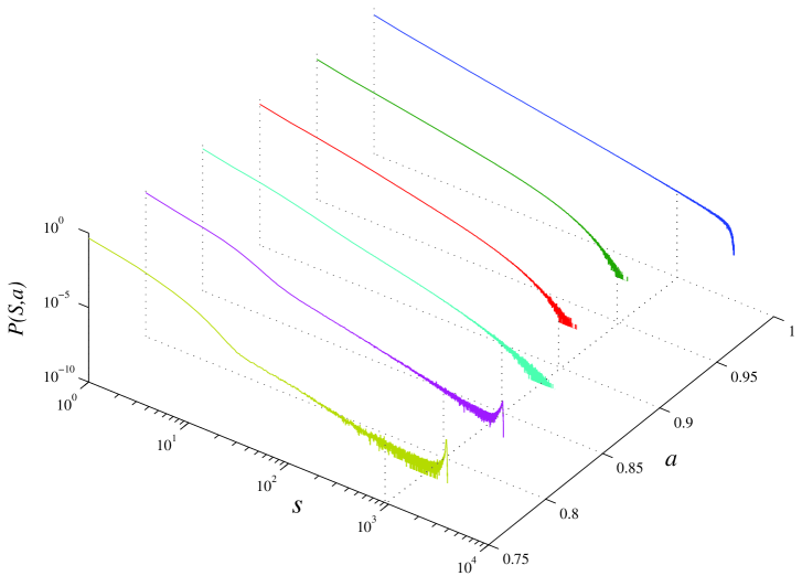
Figure 1: Distribution of avalanche sizes for different control parameter $a$, $L=64$ and $p_{add}=0$.

In Fig. 1 we plot the avalanche size distribution for the weighted OFC model with different control parameters $a$ [21]. From this figure, we find that the system develops an approximate power-law distribution for avalanche sizes in a wide range of parameter $a$. When $a\leq 0.88$, the model only produces a power-law distribution for avalanche sizes. The system not only shows power-law behavior but also satisfies the finite-size scaling in the parameter range $a=0.88$ to $a=1$.

3.2 Avalanche-Size Distribution–finite-size scaling

To verify the criticality of our weighted model, we study the effect of increasing the system size $L$. We observe that, for each constant value of $a$, the avalanche size exponent $\tau$ does not change, while the cutoff in the energy distribution scales with the system size. Our weighted OFC model not only shows power-law behavior in the avalanche size distribution, but also satisfies the finite-size scaling behavior in the parameter range mentioned above. In this part, we propose a simple finite-size scaling analysis for the avalanche size distribution of the form

$$P(S,L) \propto L^{-\beta}g(S/L^{\nu})\,\,,$$ (5)

where $g$ is the so-called universal scaling function, parameters $\beta$ and $\nu$ are critical exponents used to characterize scaling properties. $\nu$ may reflect the scaling relationship between the cut off of the distribution function and the system size, while $\beta$ is a normalization parameter. Fig. 2 displays $P(S,L)$ versus the avalanche size $S$ for the weighted OFC model on square lattice of size $L=32,48,64$ with control parameter $a=1$ and the inset of Fig. 2 displays the transformed avalanche size distribution, $L^{\beta}P(S,L)$, versus rescaled avalanche size, $S/L^{\nu}$. A clear data collapse is evident for the proposed scaling function with $\beta=2.456$, $\nu=2.002$. The value of critical avalanche size exponent ($\tau=1.220\pm 0.003$) [20] is in agreement with the finite-size scaling hypothesis since for asymptotically large $N$, it is well-known that $P(S)\sim S^{-\tau}$ with $\tau=\beta/\upsilon$ [22], which gives $\tau=1.227$ for the obtained values of $\beta$ and $\nu$. So far, we can conclude that our weighted OFC model are not only self-organized but also critical.

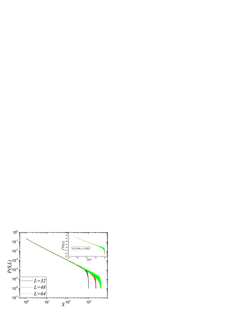
Figure 2: The avalanche size distribution $P(S,L)$ for the weighted OFC model on square lattice with system size $L=32,48,64$. In the inset, the transformed avalanche size distribution versus rescaled avalanche size is given.

3.3 Avalanche-Size Distribution–Effect of long range parameter

In this section, we mainly discuss the effects of long-range connectivity. The reasons why we introduce long range to our model must be given first. To begin with, constructing networks from real seismic data, Baiesi and Paczuski as well as Abe and Suzuki reported the discoveries of the scale-free and the small-world features in real earthquakes [8, 17, 18]. Then, according to the geophysics and geology, heterogeneous character of real earthquake systems and the effect of long-range interactions in real earthquakes were found by Mori and Kawamura [23], for instance in earthquake triggering and interaction, where the static stress may involve relaxation processes in the asthenosphere with relevant spatial and temporal long-range effects. Here, we introduce a small fraction of long-range links (denoted as the long range parameter $p_{add}$) in the lattice so as to obtain a small world topology. The long-range connections largely reduce the average distance of the original network (here, our model is based on the $NW$ small-world model).

In [20], the effects of the control parameter have mainly discussed, here we only discuss the behavior of the critical state. In this model, the state of the system is controlled by the control parameter and long rang parameter $p_{add}$. So, whether the system is in self-organized criticality or not depends on these two parameters. Depending on the long-range parameter, the network can produce a rich repertoire of behaviors. In Fig. 3, we fix $a=1$ and show examples of avalanche size distributions for various values of $p_{add}$. For small values of $p_{add}$ ($p_{add}\leq 0.3$), critical avalanche size distributions are observed. This regime is characterized by an approximate power-law distribution for avalanche sizes almost up to the system sizes where an exponential cutoff is observed. For larger values of $p_{add}$ ($p_{add}>0.3$), the distribution is supercritical, that is, a substantial fraction of triggering events spread through the whole system [21]. When the control parameter equals to other values, the system shows self-organized criticality behavior which is different from the behavior above, and this can be explained as it is on the more susceptive critical state ($a=1$) than others. In the inset of Fig. 3, we have simulated this behavior based on different lattices and found that they show the same behavior independent of lattice size expect for $L\leq 16$, which can be considered as the effects of boundary conditions.

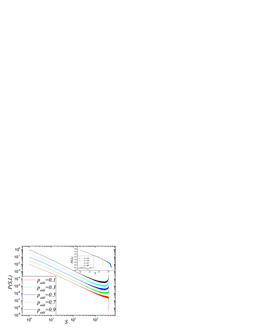
Figure 3: Avalanche size distributions for different long range parameter $p_{add}$. The long range parameter near $p_{add}\leq 0.3$ seems critical. For $p_{add}>0.3$, the distribution is supercritical. The inset shows $P(S,L)$ versus the avalanche size $S$ for the weighted OFC model on square lattice with system sizes $L=10,16,32$ and 48 for $a=0.97$ and $p_{add}=0.7$.

3.4 Probability density function for the avalanche size difference

In recent years, SOC models have been intensively studied considering time intervals between avalanches in the critical regime [24]. Here, we follow a different approach which reveals interesting information on the eventual criticality of the model under examination. Inspired by recent studies on turbulence and the time-series of real earthquakes, we introduce the distribution of returns, i.e., the differences between fluctuation lengths obtained at consecutive time steps, as $\triangle S(t)=S(t+\delta)-S(t)$, on the differences between avalanche sizes calculated at time $t+\delta$ and at time $t$, $\delta$ being a discrete time interval [25, 26, 9]. It should also be noted that, in order to have zero mean, the returns are normalized by introducing the variable $x$ as:

$$x=\triangle S-<S>$$ (6)

where $<.>$ stays for the mean value of the given data set [27]. The signal of the distribution of returns reveals very interesting results on the criticality of the weighted OFC model. In recent works [9, 28, 29], it is shown that the return distributions can be well approximated by a $q$-Gaussian of type

$$P(x)=P(0)[1-B(1-q)x^{2}]^{1/(1-q)},$$ (7)

(which are the standard distributions obtained in nonextensive statistical mechanics [30, 31] and from where the standard Gaussian form is obtained as a special case for $q\rightarrow 1$) when the avalanche size distribution is a power-law with an exponent $\tau$. Moreover, it is also found that the appropriate $q$ value could be determined a priori from the exact relation

$$q=\frac{\tau+2}{\tau}$$ (8)

given in [29]. It is clear from those efforts that, as the system size increases, the power-law regime in avalanche size distribution persists more and more (before arriving the exponential decay part) which makes the appropriate $q$-Gaussian for the return distribution to dominate more and more the tails together with the central part. On the other hand, usually it is very difficult (if not impossible) to reach very large system sizes (in order to approach thermodynamic limit) in such model systems. For the small system sizes, considerably short power-law regime is immediately followed by the exponential decay in avalanche size distribution and consequently this yields in the return distribution the appropriate $q$-Gaussian to deteriorate in the tails [29, 28].

In order to explain this tendency, a mathematical simple model for finite-size effects exhibiting the gradual approach to $q$-Gaussians, has been proposed using the following differential equation [31, 32]:

$$\frac{dy}{d(x^{2})}=-b_{r}y^{r}-(b_{q}-b_{r})y^{q}\;\;\;\;(b_{q}\geq b_{r}\geq 0;\,q>1;\,y(0)=1)\,.$$ (9)

For the particular case $r=1$, if one takes $b_{1}=0$, the solution is given by the $q$-Gaussian $y=\left[1-(1-q)b_{q}x^{2}\right]^{(1/(1-q))}\equiv e_{q}^{-b_{q}\,x^{2}}$. If $b_{q}=b_{1}$, the solution is given by the Gaussian $y=e^{-b_{1}\,x^{2}}$. For the case $b_{q}>b_{1}>0$ and $q>1$, we obtain a crossover between these two solutions, the $|x|\to\infty$ asymptotic one being the Gaussian behavior. For this particular case with $q>1$, the solution can be found as an explicit expression of the form $y(x)$, namely,

$$y=\frac{1}{\Bigl{[}1-\frac{b_{q}}{b_{1}}+\frac{b_{q}}{b_{1}}\,e^{(q-1)b_{1}\,x^{2}}\Bigr{]}^{\frac{1}{q-1}}}\,.$$ (10)

On the other hand, for the particular case $r=0$ with $q>1$, the solution can only be given by the explicit $x(y)$ form, namely,

$$x^{2}=\frac{1}{b_{0}}\Bigl{\{}\\ _{2}F_{1}\Bigl{[}\frac{1}{q},1,1+\frac{1}{q},-\frac{(b_{q}-b_{0})}{b_{0}}\Bigr{]}-\,_{2}F_{1}\Bigl{[}\frac{1}{q},1,1+\frac{1}{q},-\frac{(b_{q}-b_{0})}{b_{0}}\,y^{q}\Bigr{]}y\Bigr{\}}\,,$$ (11)

where ${}_{2}F_{1}$ is the hypergeometric function.

Indeed, the weighted OFC model studied here constitutes a very good example to check the validity of both solutions since (i) it is an example of a model which can only be simulated with small system sizes and (ii) the model allows us to define two types of avalanche definition, one of which seems to produce return distributions that can be approached by Eq.(10), whereas the other definition yields return distributions that can be given by Eq.(11). The standard way of defining an avalanche (the one also used throughout this work) is to include each triggered site only once during an avalanche which restricts the size of an avalanche with the size of the system. This definition results in the return distributions shown in Fig. 4. It is easily seen that the returns are well approximated by the crossover formula given in Eq.(11) with $q=2.64$ which comes a priori from Eq.(8). It is also evident from this figure that, as $L\rightarrow\infty$ limit is approached, it seems that the return distributions would converge to the $q$-Gaussian with $q=2.64$ for the entire region including the central part and the tails.

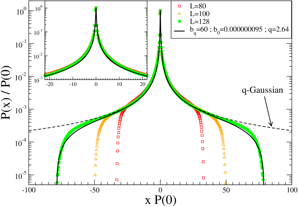
Figure 4: The probability distribution functions of the weighted OFC model with restricted avalanche definition for representative system sizes. The crossover formula given in Eq.(11) seems to describe the tendency in the entire region except the turning points in the tails (central part is given in the Inset). As system size increases, it is clearly seen that the return distributions appear to approach the prefect $q$-Gaussian curve better and better.

Another way of defining an avalanche is to relax the restriction that allows each site to trigger only once during an avalanche. This means that, during a running avalanche, one site can be triggered more than once which clearly relaxes the restriction of having maximum avalanche sizes of the order of system size. The use of such definition does not change the value of the avalanche size distribution exponent $\tau$ but results in a smoother crossover from the power-law regime to exponential decay part. This observed tendency would be expected to have an effect also in the return distributions. This can be seen in Fig. 5 where the return distributions can now be well approached by the crossover formula given in Eq.(10). The gradual approach to the perfect $q$-Gaussian is evident as the system size is increased. It is also worth noting here that the observed behavior of return distributions do not depend on the interval $\delta$ considered for the avalanche size difference, which is also the case for the worldwide and the northern California catalogs [9].

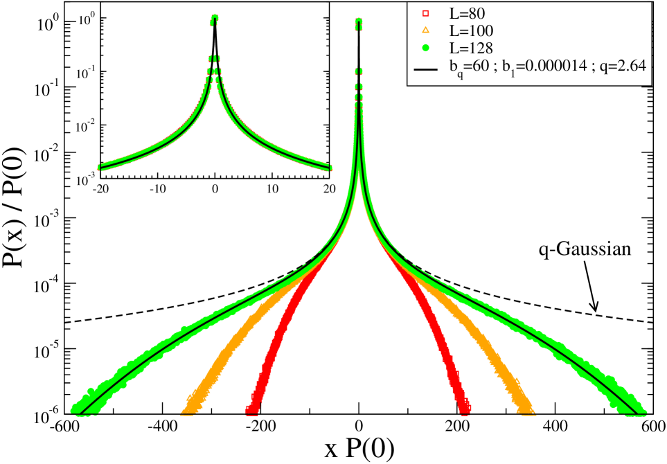
Figure 5: The probability distribution functions of the weighted OFC model with non-restricted avalanche definition for representative system sizes. The crossover formula given in Eq.(10) seems to perfectly describe the tendency in the entire region (central part is given in the Inset). As system size increases, it is clearly seen that the return distributions appear to approach the perfect $q$-Gaussian curve better and better.

As a result, one can conclude here that the behavior of the return distributions is very different from a Gaussian shape and seems to be well approached by one of the two crossover formulas (either by Eq.(10) if the non-restricted definition of avalanche is used or by Eq.(11) if the restricted definition of avalanche is used). As far as we know, this constitutes the first example in literature where the two forms of these crossover solutions can be used together in the same model system. Finally, all the numerical findings obtained here suggest that, as the thermodynamic limit is approached, the behavior of the return distributions seems to converge to the appropriate $q$-Gaussian shape in the entire region.

3.5 Statistics of waiting time in weighted OFC model

Recently, a new necessary SOC signature has been proposed, in the context of solar flare dynamics. It is based on a different type of statistics that deals with waiting times, i.e., the time intervals between two successive bursts or avalanches. In this section, we consider the waiting time of avalanche sequences generated by our weighted model. The waiting time is defined as the time between the first trigger and the second one. We use the overall statistical method and statistics of the waiting times for any node, then the distribution of all nodes. After this, we calculated probability distribution of waiting times. It can be argued that, if the triggers are not correlated, the process should be somehow related to a Poisson process, and the probability distribution function of the waiting times should be an exponential law. However,the existence of extended power laws in the waiting-time probability distribution function of solar flare measurements has been noticed by several authors [33, 34]. Several years ago, Christensen et al. showed that waiting times would follow power-law distributions if only events larger than a certain size are considered in the context of a spring-block model for earthquakes [35]. In this paper, we also analyze the waiting time distribution of the weighted OFC model which exhibits a clear nonexponential behavior as can be seen in Fig. 6. The power-law regime of the waiting time distribution lasts about two decades.

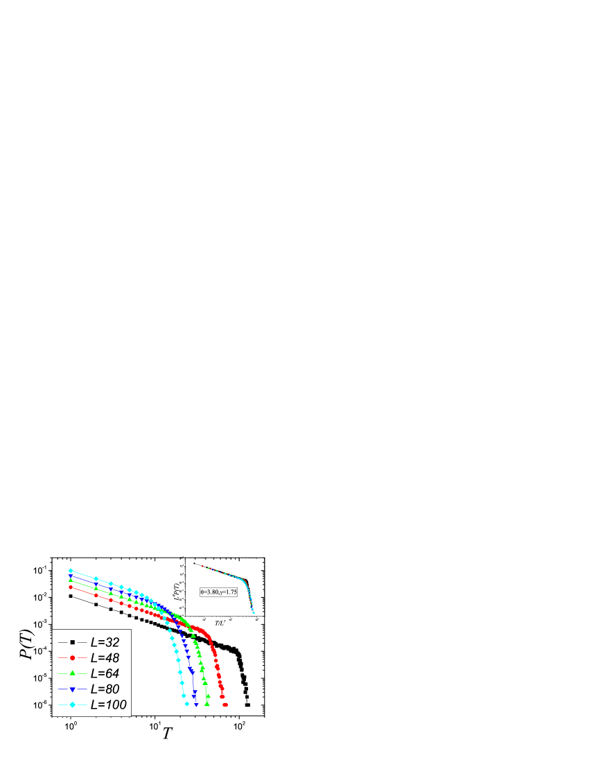
Figure 6: The waiting time distribution and its scaling analysis.

We propose a scaling relation for the waiting-time distribution of the form

$$P(T) \propto L^{-\theta}g(T/L^{\gamma})\,\,,$$ (12)

with the scaling exponents $\theta=3.80$ and $\gamma=1.75$, which are shown (see the inset of Fig. 6) to be consistent with the data coming from our model.

4 Summary and Conclusion

In order to obtain the inhomogeneous network and different local friction and elasticity, we have introduced the weighted edge to improve the original redistribution rule. We have shown self-organized criticality in the weighted coupled map lattice. The probability density functions of the avalanche size differences (namely, return distributions) appear to exhibit fat tails that can be approached by a $q$-Gaussian shape, in the thermodynamic limit, with an appropriate value of $q$ coming a priori from the avalanche size exponent $\tau$. Moreover, for the small system sizes, the observed behavior of the return distributions seems to obey the crossover formula proposed in [32] in order to explain the transition from the $q$-Gaussian behavior to the Gaussian observed so far in some other model systems with small system sizes. These results could be interpreted that there are no correlations between any two seismic behavior. Our findings support the hypothesis that even the statistical data of previous earthquake is known, the magnitude of the next earthquake is still unpredictable. Finally, the scaling relation of waiting times for the weighted OFC model has been discussed and obtained.

5 ACKNOWLEDGEMENTS

This work has been supported by the National Natural Science Foundation of China under Grant No.10675060 and by Ege University under the Research Project number 2009FEN027. We thanks C.P.Zhu and H.Kong for useful discussions.

References

- [1] P. Bak, C. Tang, and K. Wiesenfeld, Phys. Rev. Lett. , 381 (1987).
- [2] P. Bak, C. Tang, and K. Wiesenfeld, Phys. Rev. A , 364 (1988).
- [3] H. J. Jensen Self-Organized Criticality (Cambridge University Press, Cambridge, England, 1998).
- [4] P. Bak, How Nature works (Springer-Verlag, New York, USA, 1996).
- [5] R. Burridge and L. Knopoff, Bull. Seismol. Soc. Am. , 341 (1967).
- [6] Z. Olami, H. J. S. Feder, and K. Christensen, Phys. Rev. Lett. , 1244 (1992).
- [7] K. Christensen and Z. Olami, Phys. Rev. A , 1829 (1992).
- [8] S. Abe, and N. Suzuki, Eur. Phys. J. B , 115 (2005).
- [9] F. Caruso, A. Pluchino, V. Latora, S. Vinciguerra and A. Rapisarda, Phys. Rev. E , 055101(R) (2007).
- [10] K. Christensen and Z. Olami, Phys. Rev. E , 3361 (1993).
- [11] K. Christensen, Self-organization in models of sandpiles, earthquakes and flashing fireflies, Ph. D. Theis, University of Aarhus, Denmark, 1992.
- [12] B. Gutenberg and C. F. Richter, Ann. Geophys. , 1 (1956).
- [13] Z. Olami and K. Christensen, Phys. Rev. A , 1720(R) (1992).
- [14] N. Mousseau, Phys. Rev. Lett. , 968 (1996).
- [15] S. Hergarten and H. J. Neugebauer, Phys. Rev. Lett. , 238501 (2002).
- [16] F. Caruso, V. Latora, A. Pluchino, A. Rapisarda and B. Tadic, Eur. Phys. J. B , 243 (2006).
- [17] S. Abe, and N. Suzuki, Physica A , 357 (2004).
- [18] M. Baiesi and M. Paczuski, Phys. Rev. E. , 066106 (2004).
- [19] T. P. Peixoto, and J. Davidsen, Phys. Rev. E , 066107 (2008).
- [20] G.-Q. Zhang, L. Wang and T.-L. Chen, Physica A , 1249 (2009).
- [21] A. Levina, J. M. Herrmann and T. Geisel, Nature Physics , 857 (2007).
- [22] K. Christensen and N. R. Moloney, Complexity and Criticality (Imperial College Press, London, England, 2005).
- [23] T. Mori and H. Kawamura. Phys. Rev. E , 051123 (2008).
- [24] A. Corral, Phys. Rev. Lett. , 108501 (2004).
- [25] M. de Menech and A. L. Stella, Physica A , 289(2002).
- [26] C. Beck, E. G. D. Cohen and H. L. Swinney, Phys. Rev. E , 056133 (2005).
- [27] B. Bakar and U. Tirnakli, Phys. Rev. E , 040103(R) (2009).
- [28] B. Bakar and U. Tirnakli, Physica A , 3382 (2010).
- [29] A. Celikoglu, U. Tirnakli and S.M. Duarte Queiros, Phys. Rev. E , 021124 (2010).
- [30] C. Tsallis, J. Stat. Phys. , 479 (1988).
- [31] C. Tsallis, Introduction to Nonextensive Statistical Mechanics - Approaching a Complex World (Springer, New York, 2009).
- [32] C. Tsallis and U. Tirnakli, J. Phys.: Conf. Ser. , 012001 (2010).
- [33] G. Boffetta, V. Carbone, P. Giuliani, P. Veltri and A. Vulpiani, Phys. Rev. Lett. , 4662 (1999).
- [34] M. S. Wheatland, P. A. Strurrock and J. M. Mctiernan, Astrophys. J. , 448 (1998).
- [35] K. Christensen and Z. Olami, J. Geophys. Res. , 8729 (1992).