Using entropy measures for comparison of software traces

Abstract

The analysis of execution paths (also known as software traces) collected from a given software product can help in a number of areas including software testing, software maintenance and program comprehension. The lack of a scalable matching algorithm operating on detailed execution paths motivates the search for an alternative solution.

This paper proposes the use of word entropies for the classification of software traces. Using a well-studied defective software as an example, we investigate the application of both Shannon and extended entropies (Landsberg-Vedral, Rényi and Tsallis) to the classification of traces related to various software defects. Our study shows that using entropy measures for comparisons gives an efficient and scalable method for comparing traces. The three extended entropies, with parameters chosen to emphasize rare events, all perform similarly and are superior to the Shannon entropy.

I Introduction

A software execution trace is a log of information captured during a given execution run of a computer program. For example, the trace depicted in Figure 1 shows the program flow entering function f1; calling f2 from f1; f2 recursively calling itself, and eventually exiting these functions. In order to capture this information, each function in the software is instrumented to log both: entry to it and exit from it.

Ψ1 f1 entry
Ψ2 | f2 entry
Ψ3 | | f2 entry
Ψ4 | | f2 exit
Ψ5 | f2 exit
Ψ6 f1 exit
Ψ

Figure 1: An example of a trace

The comparison of program execution traces is important for a number of problem areas in software development and use. In the area of testing trace comparisons can be used to: 1) determine how well user execution paths (traces collected in the field) are covered in testing cotroneo_investigation_2007 ; elbaum_trace_2007 ; moe_using_2002 ; 2) detect anomalous behavior arising during a component’s upgrade or reuse mariani_dynamic_2007 ; 3) map and classify defects haran_applying_2005 ; podgurski_automated_2003 ; yuan_automated_2006 ; 4) determine redundant test cases executed by one or more test teams rothermel_empirical_1998 ; and 5) prioritize test cases (to maximize execution path coverage with a minimum number of test cases) elbaum_selecting_2004 ; miranskyy_usage_2007 . Trace comparisons are also used in operational profiling (for instance, in mapping the frequency of execution paths used by different user classes) moe_using_2002 and intrusion analysis (e.g., detecting deviations of field execution paths from expectations) lee_learning_1997 .

For some problems such as test case prioritization, traces gathered in a condensed form (such as a vector of executed function names or caller-callee pairs) are adequate elbaum_selecting_2004 . However for others, such as the detection of missing coverage and anomalous behavior using state machines, detailed execution paths are necessary cotroneo_investigation_2007 ; mariani_dynamic_2007 . The time required for analyzing traces can be critical. Examples of the use of trace analysis in practice include: 1) a customer support analyst may use traces to map a reported defect onto an existing set of defects in order to identify the problem’s root cause; 2) a development analyst working with the testing team may use trace analysis to identify missing test coverage that resulted in a user-observed defect.

Research Problem and Practical Motivation: To be compared and analyzed, traces must be converted into an abstract format. Existing work has progressed by representing traces as signals kuhn_exploiting_2006 , finite automata mariani_dynamic_2007 , and complex networks cai_software_2009 . Unfortunately, many trace comparison techniques are not scalable miranskyy_sift:_2008 ; davison_patent_2006 . For example the finite-state automata based kTail algorithm, when applied to representative traces, did not terminate even after 24 hours of execution cotroneo_investigation_2007 ; similar issues have been experienced with another finite-state automata algorithm, kBehavior miranskyy_sift:_2008 . These observations highlight the need for fast trace matching solutions.

Based on our experience, support personnel of a large-scale industrial application with hundreds of thousands of installations can collect tens of thousands of traces per year. Moreover, a single trace collected on a production system is populated at a rate of millions of records per minute. Thus, there is a clear need for scalable trace comparison techniques.

Solution Approach: The need to compare traces, together with a lack of reliable and scalable tools for doing this, motivated us to investigate alternate solutions. To speed up trace comparisons, we propose that a given set of traces first be filtered, rejecting those that are not going to match with the test cases, allowing just the remaining few to be compared for target purposes. The underlying assumption (based on our practical experience) is that most traces are very different, just a few are even similar, and only a very few are identical.

This strategy is implemented and validated in the Scalable Iterative-unFolding Technique (SIFT) miranskyy_sift:_2008 . The collected traces are first compressed into several levels prior to comparison. Each level of compression uses a unique signature or “fingerprint”. Starting with the highest compression level, the traces are compared, and unmatched ones are rejected. Iterating through the lower levels until the comparison process is complete leaves only traces that match at the lowest (uncompressed) level. The SIFT objective ends here. The traces so matched can then be passed on to external tools, such as the ones presented here, for further analysis such as defect or security breach identification.

The process of creating a fingerprint can be interpreted as a map from the very high dimensional space of traces to a low (ideally one) dimensional space. Simple examples of such fingerprints are 1) the total number of unique function names in a trace; and 2) the number of elements in a trace. However, while these fingerprints may be useful for our purposes, neither are sufficient. The “number of unique function names” fingerprint does not discriminate enough – many quite dissimilar traces can share the same function names called. At the other extreme, the number of elements in the trace discriminates too much – traces which are essentially similar may nonetheless have varying numbers of elements. The mapping should be such that projections of traces of different types should be positioned far apart in the resulting small space.

Using the frequency of the function names called is the next step in selecting useful traces. A natural one dimensional representation of this data is the Shannon information shannon_mathematical_1948 , mathematically identical to the entropy of statistical mechanics. Other forms of entropy/information, obeying slightly less restrictive axiom lists, have been defined aczel_measures_1975 . These extended entropies (as reviewed in davison_extended_2005 ) are indexed by a parameter $q$ which, when $q=1$ reduces them to the traditional Shannon entropy and which can be set to make them more ($q<1$) or less ($q>1$) sensitive to the frequency of rare events, improving the classification power of algorithms. Indeed, an extended Rényi entropy renyi_probability_1970 with $q=0$ (known as the Hartley entropy of information theory) applied in the context of this paper returns the “number of unique function names” fingerprint.

The entropy concept can also be extended in another way. Traces differ not only in which functions they call but in the pattern linking the call of one function with the call of another. As such it makes sense to collect not only the frequency of function calls, but also the frequency of calling given pairs, triplets, and in general $l$-tuples of calls. The frequency information assembled for these “$l$-words” can be converted into “word entropies” for further discriminatory power. In addition each record in a trace can be encoded in different ways (denoted by $c$) by incorporating various information such as a record’s function name or type.

Research Question: In this paper we study the applicability of the Shannon entropy shannon_mathematical_1948 and the Landsberg-Vedral landsberg_distributions_1998 , Rényi renyi_probability_1970 , and Tsallis tsallis_possible_1988 entropies to the comparison and classification of traces related to various software defects. We also study the effect of $q$, $l$, and $c$ values on the classification power of the entropies.

Note that the idea of using word entropies for general classification problems is not new to this paper. Similar work has been done to apply word entropy classification techniques to problems arising in biology vinga_renyi_2004 ; dehmer_hist_2011 , chemistry dehmer_hist_2011 , analysis of natural languages ebeling_word_1992 , and image processing bhandari_some_1993 . In the context of software traces, the Shannon entropy has been used to measure trace complexity Hamou-Lhadj_measuring_2008 . However, no one has yet applied word entropies to compare software traces.

The structure of the paper is as follows: in Section II we define entropies and explain the process of trace entropy calculation. The way in which entropies are used to classify traces is shown in Section III. Section IV provides a case study which describes and validates the application of entropies for trace classification, and Section V summarizes the paper.

II Entropies and Traces: definitions

In this section we describe techniques for extracting the probability of various events from traces (Section  II.1) and the way we use this information to calculate trace entropy (Section  II.2).

II.1 Extraction of probability of events from traces

A trace can be represented as a string, in which each trace record is encoded by a unique character. We concentrate on the following three character types $c$:

1. Record’s function name ($F$),

2. Record’s type ($FT$),

3. Record’s function names, type, and depth in the call tree ($FTD$).

In addition, we can generate consecutive and overlapping substrings of length $l$ from a string. We call such substrings $l$-words. For example, a string “ABCA” contains the following 2-words: “AB”; “BC”; and “CA”.

One can consider a trace as a message generated by a source with source dictionary $A=\{{a_{1}},{a_{2}},\ldots,{a_{n}}\}$ consisting of $n$ $l$-words ${a_{i}}$, $i=1,2,\ldots,n$, and discrete probability distribution $P=\{{p_{1}},{p_{2}},\ldots,{p_{n}}\}$, where ${p_{i}}$ is the probability ${a_{i}}$ is observed. To illustrate these ideas, the dictionaries $A$ and their respective probability distributions $P$ for various values of $c$ and $l$ are summarized in Table 1 for the trace shown in Figure 1.

Table 1: Dictionaries of a trace given in Figure 1

$C$	$l$	$n$	$A$	$P$
$F$	1	2	f1, f2	1/3, 2/3
$F$	2	3	f1-f2, f2-f2, f2-f1	1/5, 3/5, 1/5
$F$	3	3	f1-f2-f2, f2-f2-f2, f2-f2-f1	1/4, 1/2, 1/4
$FT$	1	4	f1-entry, f1-exit, f2-entry, f2-exit	1/6, 1/6, 1/3, 1/3
$FTD$	1	6	f1-entry-depth1, f1-exit-depth1, f2-entry-depth2,	1/6, 1/6, 1/6,
			f2-exit-depth2, f2-entry-depth3, f2-exit-depth3	1/6, 1/6, 1/6

Define a function $\alpha$ that, given a trace $t$, will return a discrete probability distribution $P$ for $l$-words of length $l$ and characters of type $c$:

$$P\leftarrow\alpha(t;l,c).$$ (1)

The above empirical probability distribution $P$ can now be used to calculate the entropy of a given trace for a specific $l$-word with type-$c$ characters. For notation convenience we suppress the dependence of $P$ (and the individual $p_{i}$’s) on the $t$, $l$, and $c$. We now define entropies and discuss how we can utilize $P$ to compute them.

II.2 Entropies and traces

The Shannon entropy shannon_mathematical_1948 is defined as

$${H_{S}}(P)=-\sum\limits_{i=1}^{n}{{p_{i}}{{\log}_{b}}{p_{i}}},$$ (2)

where $P$ is the vector containing probabilities of the $n$ states, and $p_{i}$ is the probability of $i$-th state. The logarithm base $b$ controls the units of entropy. In this paper we set $b=2$, to measure entropy in bits.

Three extended entropies, Landsberg-Vedral landsberg_distributions_1998 , Rényi renyi_probability_1970 , and Tsallis tsallis_possible_1988 are defined as:

$${H_{L}}(P;q) = \frac{{1-1/Q(P;q)}}{{1-q}},$$

$${H_{R}}(P;q) = \frac{{{{\log}_{2}}\left[{Q(P;q)}\right]}}{{1-q}},\text{ and}$$ (3)

$${H_{T}}(P;q) = \frac{{Q(P;q)-1}}{{1-q}},$$

respectively, where $q\geq 0$ is the entropy index, and

$$Q(P;q)=\sum\limits_{i=1}^{n}{p_{i}^{q}.}$$ (4)

These extended entropies reduce to the Shannon entropy (by L’Hôpital’s rule) when $q=1$. The extended entropies are more sensitive to states with small probability of occurrence than the Shannon entropy for $0<q<1$. Setting $q>1$ leads to increased sensitivity of the extended entropies to states with high probability of occurrence.

The entropy $Z$ of a trace $t$ for a given $l$, $c$, and $q$ is calculated by inserting the output of Equation (1) into one of the entropies described in Equations (2) and (II.2):

$$Z\leftarrow{H_{E}}\left[{\alpha(t;l,c);q}\right]$$ (5)

where $E\in\{L,R,T,S\}$. Note that if $E=S$ then $q$ is ignored, since in fact it must be that $q=1$.

III Using entropies for classification of traces

A typical scenario for trace comparison is the following. A software service analyst receives a phone call from a customer reporting software failure. The analyst must quickly determine the root cause of this failure and identify if 1) this is a rediscovery of a known defect exposed by some other customer in the past or 2) this is a newly discovered defect. If the first case is correct then the analyst will be able to provide the customer with a fix-patch or describe a workaround for the problem. If the second hypothesis is correct the analyst must alert the maintenance team and start a full scale investigation to identify the root-cause of this new problem. In both cases time is of the essence – the faster the root cause is identified, the faster the customer will receive a fix to the problem.

In order to validate the first hypothesis, the analyst asks the customer to reproduce the problem with a trace capturing facility enabled. The analyst can then compare the newly collected trace against a library of existing traces collected in the past (with known root-causes of the problems) and identify potential candidates for rediscovery. To identify a set of traces relating to similar functionality the library traces are usually filtered by names of functions present in the trace of interest. After that the filtered subset of the library traces is examined manually to identify common patterns with the trace of interest.

If the analyst finds an existing trace with common patterns then the trace corresponds to a rediscovered defect. Otherwise the analyst can conclude that this failure relates to a newly discovered defect. This process is similar in nature to an Internet search engine. A user provides keywords of interest and the engine’s algorithm returns a list of web pages ranked according to their relevance. The user examines the returned pages to identify her most relevant ones.

To automate this approach using entropies as fingerprints, we need an algorithm that would compare a trace against a set of traces, rank this set based on the relevance to a trace of interest, and then return the top $X$ closest traces for manual examination to the analyst. In order to implement this algorithm we need the measure of distance between a pair of traces described in Section III.1, and the ranking algorithm described in Section III.2. The algorithm’s efficiency is analyzed in Section III.3.

III.1 Measure of distance between a pair of traces

We can obtain multiple entropy-based fingerprints for a trace by varying values of $E$, $q$, $l$ and $c$. Denote a complete set of 4-tuples of $[E,q,l,c]$ as $M$. We define the distance between a pair of traces $t_{i}$ and $t_{j}$ as:

$$D({t_{i}},{t_{j}};M)=\left({\sum\limits_{k=1}^{m}{{{\left|{\frac{{{H_{{E_{k}}}}\left[{\alpha({t_{i}};{l_{k}},{c_{k}});{q_{k}}}\right]-{H_{{E_{k}}}}\left[{\alpha({t_{j}};{l_{k}},{c_{k}});{q_{k}}}\right]}}{{\max\left\{{{H_{{E_{k}}}}\left[{\alpha(t;{l_{k}},{c_{k}});{q_{k}}}\right]}\right\}}}}\right|}^{w}}}}\right)^{1/w},$$ (6)

where $m$ is the number of elements in $M$, $w$ controls the type of “norm”, $\max\left\{{{H_{{E_{k}}}}\left[{\alpha(t;{l_{k}},{c_{k}});{q_{k}}}\right]}\right\}$ denotes the maximum value of ${H_{{E_{k}}}}$ for the complete set of traces under study for a given $q_{k}$, $l_{k}$, and $c_{k}$; $k$ indexes the 4-tuple $[E_{k},q_{k},l_{k},c_{k}]$ in $M$ with $E_{k}$, $q_{k}$, $l_{k}$, and $c_{k}$ indicating the entropy, $q$, $l$-word length and character type for the $k$-th 4-tuple, $k=1,\ldots,m$.

This denominator is used as a normalization factor to set equal weights to fingerprints related to different 4-tuples in $M$.

Formula 6 satisfies three of the four usual conditions of a metric:

$$D({t_{i}},{t_{j}};M) \geq 0,$$

$$D({t_{i}},{t_{j}};M) = D({t_{j}},{t_{i}};M),$$ (7)

$$D({t_{i}},{t_{k}};M) \leq D({t_{i}},{t_{k}};M)+D({t_{k}},{t_{j}};M).$$

However, the fourth metric condition, $D({t_{i}},{t_{j}};M)=0\Leftrightarrow{t_{i}}={t_{j}}$ (identity of indiscernibles), holds true only for the fingerprints of traces; the actual traces may be different even if their entropies are the same. In other words, the identity of indiscernibles axiom only “half” holds: ${t_{i}}={t_{j}}\Rightarrow D({t_{i}},{t_{j}};M)=0,$ but $D({t_{i}},{t_{j}};M)=0\not\Rightarrow{t_{i}}={t_{j}}.$ As such, $D$ represents a pseudo-metric. Note that $D({t_{i}},{t_{j}};M)\in[0,\infty)$ and our hypothesis is the following: the larger the value of $D$, the further apart are the traces.

Note that for a single pair of entropy-based fingerprints the normalization factor in Equation (6) can be omitted and we define $D$ as

$$D({t_{i}},{t_{j}}; E ,q,l,c)=\left|{{H_{E}}\left[{\alpha({t_{i}};l,c);q}\right]-{H_{E}}\left[{\alpha({t_{j}};l,c);q}\right]}\right|.$$ (8)

Entropies have the drawback that they cannot differentiate dictionaries of events, since entropy formulas operate only with probabilities of events. Therefore, the entropies of the strings “f1-f2-f3-f1” and “f4-f5-f6-f4” will be exactly the same for any value of $E$, $l$, $c$, and $q$. The simplest solution is to do a pre-filtering of traces in $T$ in the spirit of the SIFT framework described in Section I. For example, one can filter out all the traces that do not contain “characters” (e.g., function names) present in the trace of interest before using entropy-based fingerprints.

We now define an algorithm for ranking a set of traces with respect to the trace of interest.

III.2 Traces ranking algorithm

Given a task of identifying the top $X$ closest classes of traces from a set of traces $T$ closest to trace $t$ we employ the following algorithm:

1. Calculate the distance between $t$ and each trace in $T$;

2. Sort the traces in $T$ by their distance to trace $t$ in ascending order;

3. Replace the vector of sorted traces with the vector of classes (e.g., defect IDs) to which these traces map;

4. Keep the first occurrence (i.e., the closest trace) of each class in the vector and discard the rest;

5. Calculate the ranking of classes taking into account ties using the “modified competition ranking” approach;

6. Return a list of classes with ranking smaller than or equal to $X$.

The “modified competition ranking” can be interpreted as a worst case scenario approach. The ordering of traces of equal ranks is arbitrary; therefore we examine the case when the most relevant trace will always reside at the bottom of the returned list. To be conservative, we consider the outcome in which our method returns a trace in the top $X$ positions as being in the $X$-th position.

Now consider an example of the algorithm.

III.2.1 Traces ranking algorithm: example

Assume we have five traces $t_{i}$, $i=1..5$ related to four software defects $d_{j}$, $j=1..4$ as shown in Table 2: trace $t_{5}$ relates to defect $d_{1}$; traces $t_{1}$ and $t_{3}$ relate to defect $d_{2}$; trace $t_{4}$ to defect $d_{3}$; and trace $t_{2}$ to defect $d_{4}$.

Table 2: Example: Relation between traces and defects

Defect	Trace
$d_{1}$	$t_{5}$
$d_{2}$	$t_{1},t_{3}$
$d_{3}$	$t_{4}$
$d_{4}$	$t_{2}$

Suppose that we calculate distances between traces using some distance measure. The distances between (a potentially new) trace $t$ and each trace in $T=\{t_{1},\ldots,t_{5}\}$ and the defects’ ranks obtained using these hypothetical calculations are given in Table 3. Trace $t_{2}$ is the closest to $t$, hence $d_{4}$ (to which $t_{2}$ is related) gets ranking number 1. Traces $t_{1}$ and $t_{4}$ have the same distance to $t$, therefore, $d_{2}$ and $d_{3}$ get the same rank. Based on the modified competition ranking schema algorithm we leave a gap before the set of items with the same rank and assign rank 3 to both traces. Traces $t_{3}$ and $t_{5}$ also have the same distance to $t$; however $t_{3}$ should be ignored since it relates to the already ranked defect $d_{2}$. This assigns rank 4 to $d_{1}$. The resulting sets of top $X$ traces for different values of $X$ are shown in Table 4.

Table 3: Example: Traces sorted by distance and ranked

$t_{i}$	Distance between	Class (defect ID)	Rank
	$t$ and $t_{i}$	of trace $t_{i}$
$t_{2}$	0	$d_{4}$	1
$t_{1}$	7	$d_{2}$	3
$t_{4}$	7	$d_{3}$	3
$t_{3}$	9	$d_{2}$	–
$t_{5}$	9	$d_{1}$	4

Table 4: Example: Top 1-4 defects

Top $X$	Set of defects in Top $X$
Top 1	$d_{4}$
Top 2	$d_{4}$
Top 3	$d_{4}$, $d_{2}$, $d_{3}$
Top 4	$d_{4}$, $d_{2}$, $d_{3}$, $d_{1}$

III.3 Traces ranking algorithm: efficiency

The number of operations $C$ needed by the ranking algorithm is given by

$$C = \underbrace{{\tilde{c}_{1}}O(|M||T|)}_{{\text{Step 1}}}+\underbrace{{\tilde{c}_{2}}O(|T|\log|T|)}_{{\text{Step 2}}}+\underbrace{{\tilde{c}_{3}}O(|T|)}_{{\text{Step 3}}}$$ (9)

$$+ \underbrace{{\tilde{c}_{4}}O(|T|)}_{{\text{Step 4}}}+\underbrace{{\tilde{c}_{5}}O(|T|)}_{{\text{Step 5}}}+\underbrace{{\tilde{c}_{6}}O(1)}_{{\text{Step 6}}}$$

$$\mathop{\approx}\limits^{\begin{subarray}{c}|T|\to\infty,\\ \tilde{c}_{1}\gg\{\tilde{c}_{3},\tilde{c}_{4},\tilde{c}_{5}\}\end{subarray}} \underbrace{{\tilde{c}_{1}}O(|M||T|)}_{{\text{Step 1}}}+\underbrace{{\tilde{c}_{2}}O(|T|\log|T|)}_{{\text{Step 2}}},$$

where $\tilde{c}_{i}$ is a constant number of operations associated with $i$-th step, and $|\cdot{}|$ represents the number of elements in a given set. In practice, the coefficients $\tilde{c}_{3}$, $\tilde{c}_{4}$ and $\tilde{c}_{5}$ are of much smaller order than $\tilde{c}_{1}$ and hence terms corresponding to Steps 3, 4 and 5 do not contribute significantly to $C$. The pairwise distance calculation via Equation (6) requires $O(|M|)$ operations. Therefore, calculating all distances between traces (Step 1) requires $O(|M||T|)$ operations, so for fixed $|M|$ the number of operations grows linearly with $|T|$. The average sorting algorithm, required by Step 2 (sorting of traces by their distance to trace $t$), needs $O(|T|\log|T|)$ operations cormen_introduction_2009 . Usually, ${\tilde{c}_{1}}\gg{\tilde{c}_{2}}$; this implies that a user may expect to see a linear relation between $C$ and $|T|$ (even for large $|T|$), in spite of the loglinear complexity of the second term in Equation (9).

The amount of storage needed for entropy-based fingerprints data (used by Equation (6)) is proportional to

$$\underbrace{\phi|M||T|}_{a}+\underbrace{\phi|M|}_{b}=\phi|M|(|T|+1),$$ (10)

where $\phi$ is the number of bytes needed to store a single fingerprint value. Term $a$ is the amount of storage needed for entropy-based fingerprints for all traces in $T$, and term $b$ is the amount of storage needed for the values of $\max\left\{{{H_{{E_{k}}}}\left[{\alpha(t;{l_{k}},{\tilde{c}_{k}});{q_{k}}}\right]}\right\}$ from Equation (6). Assuming that $|M|$ remains constant, the data size grows linearly with $|T|$. Now we will compare the complexity of our algorithm with an existing technique.

III.3.1 Comparison with existing algorithm

Note that a general approach for selecting a subset of closest traces to a given trace can be summarized as follows: (a) calculate the distance between $t$ and each trace in $T$; and (b) select a subset of closest traces. The principal difference between various approaches lies in the technique for calculating the distance between pairs of traces.

Suppose that the distance between a pair of traces is calculated using the Levenshtein distance levenshtein_bin_1966 . This distance can be calculated using the difference algorithm myers_diff_1986 . The worst case complexity for comparing a pair of strings using this algorithm is $O(ND_{L})$ myers_diff_1986 , where $N$ is the combined length of a pair strings and $D_{L}$ is the Levenshtein distance between these two strings. Therefore, the complexity of step (a) using this technique is $O(ND_{L})$.

Let us compare $O(ND_{L})$ with the complexity of calculating the distance using the entropy based algorithm, namely $O(|M|)$. The former depends linearly on the length of the string representation of a trace ranging between $10^{0}$ and $10^{8}$ “characters” miranskyy_sift:_2008 . However, when strings are completely different, $D_{L}=N$ and $O(ND_{L})\rightarrow O(N^{2})$, implying quadratic dependency on the trace length. Conversely, $|M|$ (representing the quantity of scalar entropy values) should range between $10^{0}$ and $10^{2}$. The computations are independent of trace size and require four mathematical function calls per scalar (see Equation (6)) when efficiently implemented on modern hardware. Therefore, our algorithm requires several orders of magnitude fewer operations than the existing algorithms.

In order to implement the Levenshtein distance algorithm we must preserve the original traces, requiring storage space for $10^{0}$ to $10^{8}$ “characters” of each trace miranskyy_sift:_2008 . An entropy based fingerprint, on the other hand, will need to store $|M|$ real numbers ($|M|$ ranging from $10^{0}$ to $10^{2}$). This represents a reduction of several orders of magnitude in storage requirements.

IV Validation case study

Our hypothesis is that the predictive classification power will vary with changes in $E$, $l$, $c$, and $q$. In order to study the classification power of ${H_{E}}\left[{\alpha(t;l,c);q}\right]$ we will analyze Cartesian products of the following sets of variables:

1. $E\in(S,L,R,T)$,

2. $l\in(1,2,\ldots,7)$,

3. $q\in(0,{10^{-5}},{10^{-4}},\ldots,{10^{1}},{10^{2}})$,

4. $c\in(F,FT,FTD)$.

We denote by $\Lambda$ the complete set of parameters obtained by the Cartesian product of the above sets.

For our validation case study we use the Siemens test suite, developed by Hutchins et al. hutchins_experiments_1994 . This suite was further augmented and made available to the public at the Software-artifact Infrastructure Repository do_supporting_2005 ; _siemens_???? . This software suite has been used in many defect analysis studies over the last decade (see jones_empirical_2005 ; murtaza_f007:_2010 for literature review) and hence provides an example on which to test our algorithm.

The Siemens suite hutchins_experiments_1994 contains seven programs. Each program has one original version and a number of faulty versions. Hutchins et al. hutchins_experiments_1994 created these faulty versions by making a single manual source code alteration to the original version. A fault can span multiple lines of source code and multiple functions. Every such fault was created to cause logical rather than execution errors. Thus, the faulty programs in the suite do not terminate prematurely after the execution of faulty code, they simply return incorrect output. Each program comes with a collection of test cases, applicable to all faulty versions and the original program. A fault can be identified if the output of a test case on the original version differs from the output of the same test case on a faulty version of the program.

In this study, we experimented with the largest program (“Replace”) of the Siemens suite. It has 517 lines of code, 21 functions, and 31 different faulty versions. There were 5542 test cases shared across all the versions. Out of these $31\times{}5542$ test cases, 4266 ($\approx 2.5\%$ of the total number of test cases) caused a program failure when exposed to the faulty program, i.e., were able to catch a defect. The remaining test cases were probably unrelated to the 31 defects. The traces for failed test cases were collected using a tool called Etrace _etrace_???? . The tool captures sequences of function-calls for a particular software execution such as the one shown in Figure 1. In other words, we collected 4266 function-call level failed traces for 31 faults (faulty versions) of the “Replace” program.

The distribution of the number of traces mapped to a particular defect (version) is given in Figure 2. Descriptive statistics of trace length are given in Table 5. The length ranges between 11 and 101400 records per trace; with an average length of 623 records per trace. Average dictionary sizes for various values of $c$ are given in Figure 3. Note that as $l$ gets larger the dictionary sizes for all $c$ start to converge.

Table 5: Descriptive statistics of length of traces

Min.	1st Qu.	Median	Mean	3rd Qu.	Max.
11	218	380	623.3	678	101400

Figure 2: Distribution of the number of traces per defect(version)

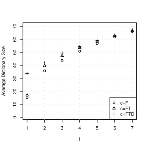
Figure 3: Dictionary size for various values of $l$ and $c$.

All of the traces contain at least one common function. Therefore, we skip the pre-filtering step. Note that direct comparison with existing trace comparison techniques is not possible since 1) the authors focus on identification of faulty functions jones_empirical_2005 ; murtaza_f007:_2010 instead of identification of defect IDs and 2) the authors jones_empirical_2005 analyze a complete set of programs in the Siemens suite while we focus only on one program (Replace).

The case study is divided as follows: the individual classification power of each ${H_{E}}\left[{\alpha(t;l,c);q}\right]$ is analyzed in Section IV.1, while Section IV.2 analyzes the classification power of the complete set of entropies. Timing analysis of the algorithm is given in Section IV.3, and threats to validity are discussed in Section IV.4.

IV.1 Analysis of individual entropies

Analysis of the classification power of individual entropies is performed using 10-fold cross-validation. In this approach the sample set is partitioned into 10 disjoint subsets of equal size. A single subset is used as validation data for testing and the remaining nine subsets are used as training data. The process is repeated tenfold (ten times) using each data subset as the validation data just once. The results of the validation from each fold are averaged to produce a single estimate. This 10-fold repetition guards against the sampling bias which can be introduced through the use of the more traditional 1-fold validation in which 70% of the data is used for training and the remaining 30% is used for testing. The validation process is designed as follows:

1. Randomly partition 4266 traces into 10 bins

2. For each set of parameters ${E,l,c,q}$

   1. For each bin

      1. Tag traces in a given bin as a validating set of data and traces in the remaining nine bins as a training set

      2. For each trace $t$ in the validating set calculate the rank of $t$’s class (defect ID) in the training set using the algorithm in Section III.2 with Equation (8) as the measure of distance and with the set of parameters ${E,l,c,q}$

   2. Compute summary statistics about ranks of the “true” classes and store this data for further analysis

Our findings show that the best results are obtained for $H$ with $E\in(L,R,T)$, $l=3$, $q\in({10^{-5}},{10^{-4}})$, and $c=FTD$. Based on 10-fold cross validation, the entropies with these parameters were able to correctly classify $\approx 21.6\%\pm 1.1\%$ of the Top 1 defects and $\approx 57.6\%\pm 1.5\%$ of the Top 5 defects (see Table 6 and Figure 4). Based on the standard deviation data in Table 6, all six entropies show robust results. However, the results become slightly more volatile for high ranks (see Figure 5). We now analyze these findings in details.

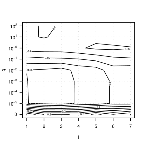
Figure 4: Interpolated average fractions of correctly classified traces in the Top 5 (based on 10-fold cross validation) for $E=L$, $l=3$, $q=10^{-5}$, and $c=FTD$ for different values of $l$ and $q$.

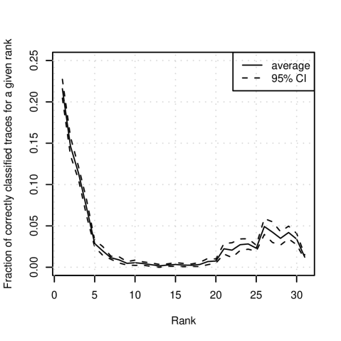
Figure 5: Fraction of correctly classified traces in the Top 5 for $E=L$ and $c=FTD$. The solid line shows the average fraction of correctly classified traces in 10 folds; the dotted line shows the pointwise $95\%$ confidence interval (95% CI) of the average.

Table 6: Fraction of correctly classified traces in Top $X$ for 1) ${H_{E}}\left[{\alpha(t;l,c);q}\right]$ with $E\in(L,R,T)$, $q\in(10^{-5},10^{-4})$, $l=3$, and $c=FTD$, and 2) set of entropies $\Lambda$; based on 10-fold cross validation. The average fraction of correctly classified traces in 10 folds is denoted by “Avg.”; plus-minus $95\%$ confidence interval is denoted by “95% CI”.

	$E$=$L$				$E$=$R$				$E$=$T$				$\Lambda{}$
Top $X$	$q$=10-4		$q$=10-5		$q$=10-4		$q$=10-5		$q$=10-4		$q$=10-5
	Avg.	95% CI	Avg.	95% CI	Avg.	95% CI	Avg.	95% CI	Avg.	95% CI	Avg.	95% CI	Avg.	95% CI
1	0.2159	0.0114	0.2159	0.0114	0.2159	0.0114	0.2159	0.0114	0.2159	0.0114	0.2159	0.0114	0.2982	0.0160
2	0.3624	0.0180	0.3624	0.0180	0.3624	0.0180	0.3624	0.0180	0.3621	0.0180	0.3621	0.0180	0.4669	0.0181
3	0.4761	0.0219	0.4761	0.0219	0.4761	0.0219	0.4761	0.0219	0.4761	0.0219	0.4761	0.0219	0.5769	0.0194
4	0.5478	0.0164	0.5478	0.0164	0.5478	0.0164	0.5478	0.0164	0.5478	0.0165	0.5478	0.0165	0.6020	0.0178
5	0.5764	0.0149	0.5764	0.0149	0.5764	0.0149	0.5764	0.0149	0.5766	0.0151	0.5766	0.0151	0.6214	0.0183
6	0.5961	0.0174	0.5961	0.0174	0.5961	0.0174	0.5961	0.0174	0.5956	0.0177	0.5956	0.0177	0.6291	0.0176
7	0.6076	0.0174	0.6076	0.0174	0.6076	0.0174	0.6076	0.0174	0.6076	0.0173	0.6076	0.0173	0.6352	0.0177
8	0.6165	0.0166	0.6165	0.0166	0.6165	0.0166	0.6165	0.0166	0.6169	0.0165	0.6169	0.0165	0.6399	0.0180
9	0.6212	0.0162	0.6212	0.0162	0.6212	0.0162	0.6212	0.0162	0.6228	0.0158	0.6228	0.0158	0.6444	0.0177
10	0.6266	0.0167	0.6266	0.0167	0.6266	0.0167	0.6266	0.0167	0.6280	0.0163	0.6280	0.0162	0.6467	0.0180
11	0.6310	0.0172	0.6310	0.0172	0.6310	0.0172	0.6310	0.0172	0.6331	0.0167	0.6331	0.0168	0.6481	0.0179
12	0.6341	0.0177	0.6341	0.0177	0.6341	0.0177	0.6341	0.0177	0.6357	0.0175	0.6357	0.0175	0.6488	0.0177
13	0.6357	0.0170	0.6357	0.0170	0.6357	0.0170	0.6357	0.0170	0.6381	0.0169	0.6381	0.0170	0.6491	0.0176
14	0.6383	0.0173	0.6383	0.0173	0.6383	0.0173	0.6383	0.0173	0.6406	0.0170	0.6406	0.0169	0.6493	0.0176
15	0.6416	0.0164	0.6416	0.0164	0.6420	0.0162	0.6416	0.0164	0.6432	0.0162	0.6432	0.0162	0.6500	0.0174
16	0.6441	0.0167	0.6441	0.0167	0.6441	0.0167	0.6441	0.0167	0.6453	0.0166	0.6453	0.0166	0.6505	0.0173
17	0.6463	0.0157	0.6465	0.0157	0.6463	0.0157	0.6465	0.0157	0.6474	0.0156	0.6477	0.0155	0.6516	0.0168
18	0.6495	0.0147	0.6498	0.0146	0.6495	0.0147	0.6498	0.0146	0.6509	0.0144	0.6512	0.0144	0.6542	0.0161
19	0.6563	0.0150	0.6566	0.0149	0.6563	0.0150	0.6566	0.0149	0.6577	0.0147	0.6580	0.0147	0.6570	0.0156
20	0.6641	0.0163	0.6641	0.0163	0.6641	0.0163	0.6641	0.0163	0.6655	0.0161	0.6655	0.0160	0.6641	0.0159
21	0.6863	0.0142	0.6863	0.0142	0.6863	0.0142	0.6863	0.0142	0.6873	0.0141	0.6873	0.0142	0.6725	0.0176
22	0.7070	0.0106	0.7070	0.0106	0.7070	0.0106	0.7070	0.0106	0.7079	0.0104	0.7079	0.0104	0.6971	0.0171
23	0.7342	0.0117	0.7342	0.0117	0.7339	0.0117	0.7339	0.0117	0.7342	0.0114	0.7342	0.0112	0.7178	0.0158
24	0.7623	0.0092	0.7623	0.0092	0.7623	0.0092	0.7623	0.0092	0.7628	0.0089	0.7628	0.0088	0.7527	0.0124
25	0.7853	0.0076	0.7853	0.0076	0.7855	0.0074	0.7855	0.0074	0.7865	0.0072	0.7865	0.0072	0.7834	0.0134
26	0.8345	0.0082	0.8345	0.0082	0.8347	0.0077	0.8347	0.0077	0.8352	0.0082	0.8352	0.0082	0.8141	0.0078
27	0.8769	0.0097	0.8769	0.0097	0.8772	0.0097	0.8772	0.0097	0.8776	0.0097	0.8776	0.0097	0.8591	0.0109
28	0.9119	0.0082	0.9119	0.0082	0.9119	0.0082	0.9119	0.0082	0.9142	0.0083	0.9142	0.0083	0.9140	0.0126
29	0.9538	0.0054	0.9538	0.0054	0.9538	0.0054	0.9538	0.0054	0.9550	0.0054	0.9550	0.0059	0.9618	0.0068
30	0.9878	0.0027	0.9878	0.0027	0.9878	0.0027	0.9878	0.0027	0.9887	0.0027	0.9887	0.0027	0.9988	0.0014
31	1.0000	0.0000	1.0000	0.0000	1.0000	0.0000	1.0000	0.0000	1.0000	0.0000	1.0000	0.0000	1.0000	0.0000

The $3$-words ($l=3$) provide the best results based on the fraction of correctly classified traces in the Top 5 (see Figure 6), suggesting that chains of three events provide an optimal balance between the amount of information in a given $l$-word and the total number of words. As $l$ gets larger, the amount of data becomes insufficient to obtain a good estimate of the probabilities.

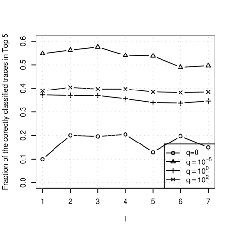
Figure 6: The average fraction of traces correctly classified in the Top 5 for various values of $l$; $E=L$, $q\in(0,{10^{-5}},{10^{0}},{10^{2}})$, $c=FTD$.

Examining the classification performance of $c$ (see Table 7) we see essentially no differences across the three levels of $c$ ($F,FT$, and $FTD$) considered here (with $E=L,l=3$, and $q\in\{10^{-4},10^{-5}\}$). This is true across all values of $X$ in the percentage of correctly classified traces in the Top $X$. This is somewhat surprising since $c=FTD$ contains more information than $c=FT$ which, in turn, contains more information than $c=F$. This suggests that for this data set and parameters ($E=l$, $l=3$, and $q\in\{10^{-4},10^{-5}\}$) the function names contain the relevant classification information, the function type (entry or exit) and depth providing no additional relevant information. Note that even though more time is needed to calculate the $FTD$-based entropies (since the dictionary of $FTD$s will contain twice as many entries as the dictionary of $FT$s) the comparison time remains the same (since the probabilities of $l$-words, $P$, map to a scalar value via the entropy function for all values of $c$).

Table 7: Percent of correctly classified traces in Top $X$ for ${H_{E}}\left[{\alpha(t;l,c);q}\right]$, $E=L$, $l=3$, and $q=\{10^{-4},10^{-5}\}$.

Top $X$	$c=F$	$c=FT$	$c=FTD$
Top 1	21.7%	20.9%	21.6%
Top 2	37.2%	35.3%	36.2%
Top 3	49.5%	46.7%	47.6%
Top 4	54.0%	53.5%	54.8%
Top 5	56.2%	56.6%	57.6%

Our findings show that the extended entropies outperform the Shannon entropy for $q<1$ and $q>1$ (see Figure 7). However, performance of extended entropies with $q<1$ is significantly better than with $q>1$, suggesting that rare events are more important than frequent events for classification of defects in this dataset. The best results are obtained for $q=10^{-4}$ and $q=10^{-5}$.

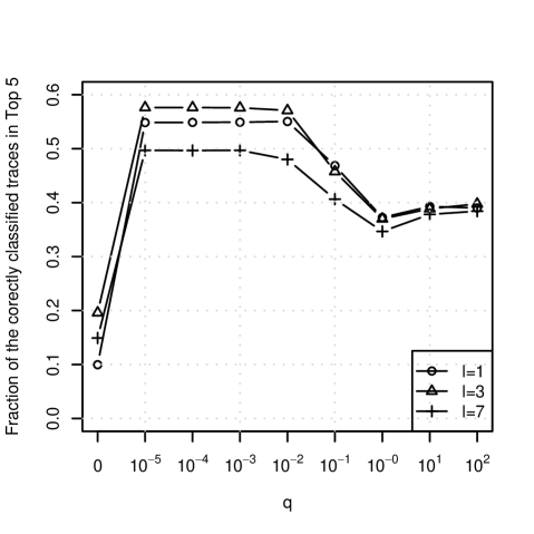
Figure 7: Average fraction of correctly classified traces in the Top 5 for various values of $q$; $E=L$, $l\in(1,3,7)$, $c~{}=~{}FTD$.

It is interesting to note that classification performance is almost identical for $H$ with $E\in(L,R,T)$, $l$=3, $q\in({10^{-5}},{10^{-4}})$, and $c=FTD$. We believe that this fact can be explained as follows: the key contribution to the ordering of similar traces (with similar dictionaries) for entropies with $q\to 0$ is affected mainly by a function of probabilities of traces’ events. This function is independent of $E$ and $q$ and depends only on $l$ and $c$, see Appendix B for details.

IV.2 Analysis of the complete set of entropies

Analysis of the classification power for the complete set of entropies is performed using 10-fold cross-validation in a similar manner to the process described in Section IV.1. However, instead of calculating distances for each $H$ independently, we now calculate distances between traces by utilizing values of $H$ for all parameter sets in $\Lambda$ simultaneously. The validation process is designed as follows

1. Randomly partition 4266 traces into 10 bins

   1. For each bin

      1. Tag traces in a given bin as a validating set of data and traces in the remaining nine bins as a training set

      2. For each trace $t$ in the validating set calculate the rank of $t$’s class (defect ID) in the training set using the algorithm in Section III.2 with Equation (6) and all 4-tuples of parameters in $\Lambda$. (Based on the experiments described in Appendix A we set $w=1$.)

   2. Compute summary statistics about ranks of the “true” classes and store this data for further analysis

The results, in the two right-most columns of Table 6, show the increase of predictive power: in the case of the Top 1 the results improved from 21.6% (for individual entropies) to 29.8% (for all entropies combined); for the Top 5 from 57.6% to 62.1%. However, the 503-fold increase in computational effort (the number of entropy fingerprints rise from 1 to 504) yielded only an 8% increase in the power to predict Top 5 matches. We leave the resulting balance between cost and benefit for each individual analyst to make.

IV.3 Timing

We compared the theoretical efficiency of our algorithm with existing algorithms in Section III.3.1. These findings may be validated against experimental timing data. We measured the time needed to compare a reference trace against a complete set of traces using difference myers_diff_1986 and entropy-based algorithms. The experiment is repeated three times for three reference traces: small (498 characters), medium (2339 characters), and large (20767 characters). The results are given in Table 8. As expected, the difference-based algorithm comparison time increases in proportion to the length of the reference trace, while the comparison time of the entropy-based algorithms remains constant across trace sizes. Moreover, the comparison time of entropy-based algorithms is several orders of magnitude faster than of the difference-based approach. Note that, even though the computational efforts for measuring distance based on the complete set of fingerprints increases by two orders of magnitude as compared to individual entropies, the results are obtained in less than a second. Therefore, from a practical perspective, we can still use a complete set of entropies for our analysis.

Table 8: Timing results (in seconds) for comparison of a single reference trace against a set of traces using difference and entropy algorithms.

	Reference trace
Algorithm	Small	Medium	Large
	(498 characters)	(2339 characters)	(20767 characters)
Difference	2.7E1	4.2E1	1.9E2
Individual entropy	1.3E-4	1.3E-4	1.3E-4
Complete set of entropies	6.8E-2	6.8E-2	6.8E-2

IV.4 Threats to Validity

A number of tests are used to determine the quality of case studies. In this section we discuss four core tests: construct, internal, statistical, and external validity yin_case_2003 . The discussion highlights potential threats to validity of our case study and tactics that we used to mitigate the threats.

Construct validity: to overcome potential construct validity issues we use two measures of classification performance (Top 1 and Top 5 correctly classified traces). Internal validity: to prevent data gathering issues all data collection was automated and a complete corpus of test cases was analyzed. Statistical validity: to prevent sampling bias, 10-fold cross validation was used. External validity: This case study shows that the method can be successfully applied to a particular, well-studied, data set. Following the paradigm of the “representative” or “typical” case advanced in yin_case_2003 , this suggests that the method may also be useful in more situations.

V Summary

In this work we analyze the applicability of a technique which uses entropies to perform predictive classification of traces related to software defects. Our validating case study shows promising performance of extended entropies with emphasis on rare events $\left({q\in\left\{10^{-5},10^{-4}\right\}}\right)$. The events are based on triplets (3-words) of “characters” incorporating information about function name, depth of function call, and type of probe point ($c=FTD$).

In the future, we are planning to increase the number of datasets under study, derive additional measures of distance (e.g., using tree classification algorithms) and identify an optimal set of parameter combinations.

Appendix A Selection of $w$ for Equation (6)

We do not have a theoretical rationale for selection of the optimal value of $w$ in Equation (6). When $|M|=1$, Equation (6) simplifies to Equation (8), becoming independent of $w$. However, in the general case of $|M|>1$, $w$ will affect performance of the distance metrics. In order to select an optimal value of $w$ we performed the analysis of the complete set of entropies discussed in Section IV.2 for $w=1,2,\ldots,5$. Table 9 gives the percentage of correctly classified traces in the Top 1 and the Top 5. The quality of classification does not change significantly with $w$. It degrades with increased $w$, but the small magnitude of this change makes us unwilling to consider it a result of the paper.

Table 9: Percent of correctly classified traces in Top $X$ for the complete set of entropies $\Lambda$ and $w=1,2,\ldots,5$.

$w$	1	2	3	4	5
Top 1	29.8%	29.7%	29.6%	29.3%	29.2%
Top 5	62.1%	61.5%	61.5%	61.3%	61.4%

Appendix B Approximation of Equation (8)

We have observed that the classification power of the ${H_{E}}\left[{\alpha(t;l,c);q}\right]$ metric is highest when $q\to 0$. In order to explain this phenomenon we expand ${H_{E}}\left[{\alpha(t;l,c);q}\right]$ (given in Equation (II.2)) in a Taylor series:

$${H_{L}}\left[{\alpha({t_{i}};l,c);q}\right] \mathop{=}\limits^{q\to 0} 1-\frac{1}{{{n_{i}}}}+q\left(\frac{{{A_{i}}}}{{n_{i}^{2}}}+\frac{{{n_{i}}-1}}{{{n_{i}}}}\right)+O({q^{2}}),$$

$${H_{R}}\left[{\alpha({t_{i}};l,c);q}\right] \mathop{=}\limits^{q\to 0} {\log_{2}}({n_{i}})$$

$$+ q\left[{\frac{{{A_{i}}}}{{\ln(2){n_{i}}}}+{{\log}_{2}}({n_{i}})}\right]+O({q^{2}}),\text{ and}$$

$${H_{T}}\left[{\alpha({t_{i}};l,c);q}\right] \mathop{=}\limits^{q\to 0} {n_{i}}-1+q\left({{A_{i}}+n-1}\right)+O({q^{2}}),$$

where $A_{i}=\sum\limits_{k=1}^{{n_{i}}}{\ln({p_{k}})}$. By plugging (B) into Equation (8) and assuming that for similar traces $n\approx{n_{i}}\approx{n_{j}}$, we get:

$$D({t_{i}},{t_{j}};L,q,l,c) \approx \frac{q}{{{n^{2}}}}\left|{{A_{i}}-{A_{j}}}\right|,$$

$$D({t_{i}},{t_{j}};R,q,l,c) \approx \frac{q}{{\ln(2)n}}\left|{{A_{i}}-{A_{j}}}\right|,\text{ and}$$ (12)

$$D({t_{i}},{t_{j}};T,q,l,c) \approx q\left|{{A_{i}}-{A_{j}}}\right|.$$

Equation (B) can be interpreted as follows. In the case in which $q\to 0$ and the dictionaries for each trace in the pair are similar, the key contribution to the measure of distance is coming from the $\sum_{k=1}^{n_{i}}{\ln({p_{k}})}$ term (which depends only on $l$ and $c$) making the rest of the variables irrelevant ($q$ and $n$ become parts of scaling factors). This can be highlighted by solving a system of equations to identify conditions that generate the same ordering for three traces ${t_{i}},{t_{j}},{t_{k}}$ for all extended entropies (using approximations from (B)):

$$\left\{\begin{gathered}\frac{q}{{{n^{2}}}}\left|{{A_{i}}-{A_{j}}}\right|\leqslant\frac{q}{{{n^{2}}}}\left|{{A_{i}}-{A_{k}}}\right|\\ \frac{q}{{\ln(2)n}}\left|{{A_{i}}-{A_{j}}}\right|\leqslant\frac{q}{{\ln(2)n}}\left|{{A_{i}}-{A_{k}}}\right|\\ q\left|{{A_{i}}-{A_{j}}}\right|\leqslant q\left|{{A_{i}}-{A_{k}}}\right|\\ \end{gathered}\right.\Rightarrow$$ (17)

$$\Rightarrow\left|{{A_{i}}-{A_{j}}}\right|\leqslant\left|{{A_{i}}-{A_{k}}}\right|.$$

In information theory $\ln(p_{k})$ measures the “surprise” (in bits) in receiving symbol $k$ which is received with probability $p_{k}$. Thus $\sum_{k=1}^{n_{i}}{p_{k}\ln(p_{k})}$ is the expected surprise or information (Shannon entropy). What about just $\sum_{k=1}^{n_{i}}{\ln(p_{k})}$? It scales with the total number of bits needed to specify each symbol. This is related to the problem of simulating processes in the presence of rare events, see rubinshtein_optimization_1997 for details.

References

- (1) J. Aczél and Z. Daróczy. On measures of information and their characterizations. Academic Press, 1975.
- (2) D. Bhandari and N. R. Pal. Some new information measures for fuzzy sets. Information Sciences, 67(3):209–228, 1993.
- (3) K.-Y. Cai and B.-B. Yin. Software execution processes as an evolving complex network. Information Sciences, 179(12):1903–1928, 2009.
- (4) T. H. Cormen, C. E. Leiserson, R. L. Rivest, and C. Stein. Introduction to Algorithms. The MIT Press, 3rd edition, 2009.
- (5) D. Cotroneo, R. Pietrantuono, L. Mariani, and F. Pastore. Investigation of failure causes in workload-driven reliability testing. In Proceedings of the 4th international workshop on software quality assurance: in conjunction with the 6th ESEC/FSE joint meeting, pages 78–85, 2007.
- (6) M. Davison, M. S. Gittens, D. R. Godwin, N. H. Madhavji, A. V. Miranskyy, and M. F. Wilding. Computer software test coverage analysis. US Patent: 7793267, 2006.
- (7) M. Davison and J. S. Shiner. Extended entropies and disorder. Advances in Complex Systems (ACS), 8(01):125–158, 2005.
- (8) M. Dehmer and A. Mowshowitz. A history of graph entropy measures. Information Sciences, 181(1):57–78, January 2011.
- (9) H. Do, S. Elbaum, and G. Rothermel. Supporting controlled experimentation with testing techniques: An infrastructure and its potential impact. Empirical Software Engineering, 10(4):405–435, 2005.
- (10) W. Ebeling and G. Nicolis. Word frequency and entropy of symbolic sequences: a dynamical perspective. Chaos, Solitons and Fractals, 2(6):635–650, 1992.
- (11) S. Elbaum, S. Kanduri, and A. Andrews. Trace anomalies as precursors of field failures: an empirical study. Empirical Software Engineering, 12(5):447–469, 2007.
- (12) S. Elbaum, G. Rothermel, S. Kanduri, and A. G. Malishevsky. Selecting a Cost-Effective test case prioritization technique. Software Quality Control, 12(3):185–210, 2004.
- (13) Etrace. http://ndevilla.free.fr/etrace/, Accessed: October 20, 2010.
- (14) A. Hamou-Lhadj. Measuring the complexity of traces using shannon entropy. In Proceedings of the Fifth International Conference on Information Technology: New Generations, pages 489–494, 2008.
- (15) M. Haran, A. Karr, A. Orso, A. Porter, and A. Sanil. Applying classification techniques to remotely-collected program execution data. In Proceedings of the 10th European software engineering conference held jointly with 13th ACM SIGSOFT international symposium on Foundations of software engineering, pages 146–155, 2005.
- (16) M. Hutchins, H. Foster, T. Goradia, and T. Ostrand. Experiments of the effectiveness of dataflow- and controlflow-based test adequacy criteria. In Proceedings of the 16th International Conference on Software Engineering, pages 191–200, 1994.
- (17) J. A. Jones and M. J. Harrold. Empirical evaluation of the tarantula automatic fault-localization technique. In Proceedings of the 20th IEEE/ACM international Conference on Automated software engineering, pages 273–282, 2005.
- (18) A. Kuhn and O. Greevy. Exploiting the analogy between traces and signal processing. In Proceedings of the 22nd IEEE International Conference on Software Maintenance, pages 320–329, 2006.
- (19) P. T. Landsberg and V. Vedral. Distributions and channel capacities in generalized statistical mechanics. Physics Letters A, 247(3):211–217, Oct. 1998.
- (20) W. Lee, S. J. Stolfo, and P. K. Chan. Learning patterns from unix process execution traces for intrusion detection. In Proceedings of the AAAI Workshop on AI Approaches to Fraud Detection and Risk Management, pages 50–56, 1997.
- (21) V. Levenshtein. Binary codes capable of correcting deletions, insertions, and reversals. Soviet Physics – Doklady, 10(8):707–710, 1966.
- (22) L. Mariani and M. Pezzé. Dynamic detection of COTS component incompatibility. IEEE Software, 24(5):76–85, 2007.
- (23) A. V. Miranskyy, M. S. Gittens, N. H. Madhavji, and C. A. Taylor. Usage of long execution sequences for test case prioritization. In Supplemental Proceedings of the 18th IEEE International Symposium on Software Reliability Engineering, 2007.
- (24) A. V. Miranskyy, N. H. Madhavji, M. S. Gittens, M. Davison, M. Wilding, D. Godwin, and C. A. Taylor. SIFT: a scalable iterative-unfolding technique for filtering execution traces. In Proceedings of the 2008 conference of the center for advanced studies on collaborative research, pages 274–288, 2008.
- (25) J. Moe and D. A. Carr. Using execution trace data to improve distributed systems. Software: Practice and Experience, 32(9):889–906, 2002.
- (26) S. S. Murtaza, M. Gittens, Z. Li, and N. H. Madhavji. F007: finding rediscovered faults from the field using function-level failed traces of software in the field. In Proceedings of the 2010 Conference of the Center for Advanced Studies on Collaborative Research, pages 57–71, 2010.
- (27) E. W. Myers. An O(ND) difference algorithm and its variations. Algorithmica, 1:251–266, 1986.
- (28) A. Podgurski, D. Leon, P. Francis, W. Masri, M. Minch, J. Sun, and B. Wang. Automated support for classifying software failure reports. In Proceedings of the 25th International Conference on Software Engineering, pages 465–475, 2003.
- (29) A. Rényi. Probability theory. North-Holland Pub. Co., 1970.
- (30) G. Rothermel, M. J. Harrold, J. Ostrin, and C. Hong. An empirical study of the effects of minimization on the fault detection capabilities of test suites. In Proceedings of the International Conference on Software Maintenance, page 34, 1998.
- (31) R. Y. Rubinstein. Optimization of computer simulation models with rare events. European Journal of Operational Research, 99:89–112, 1997.
- (32) C. E. Shannon. A mathematical theory of communication. Bell System Technical Journal, 27:623–656, 1948.
- (33) Siemens suite. http://pleuma.cc.gatech.edu/aristotle/Tools/subjects/, Accessed: October 20, 2010.
- (34) C. Tsallis. Possible generalization of Boltzmann-Gibbs statistics. Journal of Statistical Physics, 52(1):479–487, July 1988.
- (35) S. Vinga and J. S. Almeida. Rényi continuous entropy of DNA sequences. Journal of Theoretical Biology, 231(3):377–388, December 2004.
- (36) R. K. Yin. Case Study Research: Design and Methods, Applied Social Research Methods Series, Vol 5. Sage Publications, Inc, 3rd edition, 2003.
- (37) C. Yuan, N. Lao, J. Wen, J. Li, Z. Zhang, Y. Wang, and W. Ma. Automated known problem diagnosis with event traces. In Proceedings of the 1st ACM SIGOPS/EuroSys European Conference on Computer Systems 2006, pages 375–388, 2006.