Statistics and Universality in Simplified Models of Planetary Formation

Abstract

In this paper, we modify Laskar’s simplified model of planetary evolution and accretion to account for the full conservation of the total angular momentum of the system, and extend it to incorporate an accretion probability that depends on the mass and relative velocity of the colliding particles. We present statistical results for the mass and eccentricity of the planets formed, in terms of their semi-major axes, for a large number of realizations of different versions of the model. In particular, we find that by combining the mass-dependent accretion probability and the velocity-selection mechanism, the planets formed display a systematic occurrence at specific locations. By introducing properly scaled variables, our results are universal with respect to the total angular momentum of the system, the mass of the planetesimal disc, and the mass of the central star.

1 Introduction

Essentially, all models are wrong, but some are useful.

Box & Draper (1987)

Recent advances in the understanding of the final stages of the formation of the Solar System within the Nice model, have achieved, among others, reproducing the architecture of the outer part to an unprecedented level (Tsiganis et al., 2005; Morbidelli et al., 2007, 2009). In the ‘first’ Nice model (Tsiganis et al., 2005), the initial conditions are defined such that Jupiter is close to its actual position, Saturn is placed just below the semi-major axis corresponding to the 1:2 mean-motion resonance with Jupiter, and the icy giants are placed in the intervals 11–13 AU (Uranus) and 13.5–17 AU (Neptune); the planetary masses are the current ones. In addition, the Nice model assumes a 30–50 M_⊕ planetesimal disc placed beyond the initial orbit of Neptune which ends between 30–35 AU. The planetesimal disc transfers angular momentum to the planets making them migrate (Fernández & Ip, 1984; Malhotra, 1995), allowing Jupiter and Saturn to cross their mutual 1:2 mean-motion resonance. This event increases their eccentricities and induces secular resonances on the icy giants. There is a period of crossing orbits which eventually scatters the icy giants outwards, which enter the planetesimal disc (Levinson & Morbidelli, 2003). The icy giants eject inwards some planetesimals to Jupiter and Saturn, which makes them migrate even further away. The planets finish their migration once the planetesimal disc is completely depleted. The final configuration of the first Nice model is close to the observed values for both the semi-major axes and the mean eccentricities of the planets (Tsiganis et al., 2005). Recently, Morbidelli et al. (2009) extended their original results showing that encounters of Saturn with an ice giant lead to the correct secular evolution for the eccentricities of Jupiter and Saturn, and not the passage through the 1:2 mean-motion resonance, as it was originally proposed.

An important open issue in the Nice model is related to explain the initial conditions assumed in the model, from earlier stages of the formation. This question has been recently investigated, assuming an earlier multi-resonant configuration for the already formed giant planets, besides pushing the planets into such configuration, by introducing additionally semi-major axis and eccentricity decay (Batygin & Brown, 2010). Yet, the issue remains to explain those initial conditions.

The aim of this paper is to study the statistics of the final configurations of planetary systems for some models of planetary accretion and evolution, which are based on a model originally introduced by Laskar (2000a). The final orbital parameters we obtain could be used as the initial conditions for detailed calculations on the planetary evolution, e.g., aimed to describe the architecture of the planetary systems formed in the spirit of the Nice model, or to address the dynamical stability of these systems in statistical terms. Yet, it is not our purpose to obtain an accurate comparison with the initial conditions of the Nice model, or with the architecture of the Solar System. Our aim is to understand the consequences of incorporating in a simple form some important physical effects on the accretion processes. The variations of Laskar’s model included account for the systematic conservation of the total angular momentum of the system, and incorporate mass- and velocity-selection mechanisms that tune the accretion probability; note that Laskar’s model actually conserves the angular momentum, but not the methodological procedure used to achieve a fixed final angular momentum deficit (AMD). These aspects were not considered in Laskar’s model, though they constitute important building blocks of the current planetary formation theories (Safronov, 1972; Polack et al., 1996; Armitage, 2010). By comparing the outcome of the mechanisms that we include, we are able to relate them, in a statistical sense, to certain effects manifested by the final configurations. This is done directly by correlating the masses and semi-major axes of the planets formed in a large number of realizations of the models. Our results indicate a power-law behaviour of the mass in terms of the semi-major axis, whose exponent depends on the different models, and on the initial linear mass-density distribution assumed. In particular, we show that including both mass- and velocity-selection mechanisms leads to the systematic appearance of planets in certain specific locations. Moreover, by introducing properly-scaled variables, we show that these results are universal with respect to the total angular momentum of the system, the mass of the planetesimal disc and the mass of the central star.

The paper is organised as follows: In Section 2 we describe Laskar’s simplified model of planetary evolution and accretion in detail, clarify its predictions, and outline a short critique aimed to motivate the variations that we incorporate in the model. Specific details of the variations we implement and the corresponding numerical results are described in Section 3. In Section 4 we address how variations of the total angular momentum of the system, the mass of the planetesimal disc, and the mass of the central star affect our results. Finally, in Section 5 we summarise our results and conclusions.

2 A simplified model of planetary formation and evolution

2.1 The model

Laskar’s simplified model of planetary formation and evolution (Laskar, 2000a, b) considers a system which consists of one large central body of mass $M_{0}$ and a large number of particles of small mass $m_{i}$, $i=1\dots N$ ($N\gg 1$), that interact under their mutual gravitational attraction. The Hamiltonian of this $(N+1)$–body problem, in a heliocentric frame, can be written as $H=H_{0}+H_{1}$, where $H_{0}$ and $H_{1}$ are given by

$$H_{0} = \sum_{i=1}^{N}\Big{[}\frac{{\mathbf{p}}_{i}^{2}}{2m_{i}}-\frac{{\cal G}M_{0}m_{i}}{r_{i}}\Big{]},$$ (1)

$$H_{1} = \frac{1}{2M_{0}}{\mathbf{P}}^{2}_{0}-\sum_{1\leq i<j}^{N}\frac{{\cal G}m_{i}m_{j}}{r_{ij}}.$$ (2)

Here, ${\cal G}$ is the gravitational constant, $r_{i}$ is the mutual distance between the $i$-th planetesimal and the central star, $r_{ij}$ is the distance between the $i$-th and $j$-th planetesimals, ${\mathbf{P}}_{0}=-\sum_{i=1}^{N}{\mathbf{p}}_{i}$ and ${\mathbf{p}}_{i}$ are the canonical momenta associated with the star and the planetesimals, respectively. Clearly, $H_{0}$ corresponds to $N$ independent two-body Kepler problems among each planetesimal and the star, and $H_{1}$ is the perturbing term, which includes the mutual gravitational interaction among the planetesimals and the indirect term. Laskar’s model is formulated for the spatial problem; the numerical simulations are illustrated for the planar case. From now on, we focus on the latter case considering coplanar orbits.

The dynamics of $H_{0}$ is completely integrable: For each planetesimal the energy $E_{i}=-\mu m_{i}/(2a_{i})$ and the barycentric angular momentum $l_{i}=m_{i}[\mu a_{i}(1-e_{i}^{2})]^{1/2}$ ($\mu={\cal G}M_{0}$) are conserved quantities. This implies the conservation (for $H_{0}$) of the semi-major axis $a_{i}$ and eccentricity $e_{i}$ of the elliptic orbits of the planetesimals. The non-integrable character of $H$ is manifested in the long-term evolution and is due to the perturbing terms of $H_{1}$. To model these non-integrable effects, Laskar (2000a) considers the secular system, where the equations of motion are averaged over the mean longitudes. This simplification is tantamount to excluding effects related with mean-motion resonances.

Firstly, considering the case without collisions, the averaged system conserves the energy of each planetesimal, but exhibits a slow chaotic diffusion of the individual eccentricities $e_{i}$. This chaotic diffusion is constrained by the conservation of the total angular momentum of the system

$$L_{\rm tot}=\sum_{i=1}^{N}l_{i}=\sum_{i=1}^{N}m_{i}[\mu a_{i}]^{1/2}(1-e_{i}^{2})^{1/2}.$$ (3)

Including the conservation of the energy, this leads to the conservation of the total angular momentum deficit (AMD) of the system. The latter is expressed as

$$C_{\rm tot}=\sum_{i=1}^{N}C_{i}=\sum_{i=1}^{N}m_{i}[\mu a_{i}]^{1/2}[1-(1-e_{i}^{2})^{1/2}].$$ (4)

Physically, the total AMD of a planetary system is a measure of the circularity of the planetary orbits, since for small eccentricities $C_{i}\sim m_{i}[\mu a_{i}]^{1/2}e_{i}^{2}$. Conversely, large values of $C_{\rm tot}$ indicate the possibility of planetary collisions.

Pair-wise collisions in this simplified model are assumed to be totally inelastic and lead to accretion. Assuming that mass and linear momentum are conserved in the collision, $m_{i\oplus j}=m_{i}+m_{j}$ and ${\mathbf{p}}_{i\oplus j}={\mathbf{p}}_{i}+{\mathbf{p}}_{j}$, the conservation of the angular momentum follows. From these conservation laws, the orbital elements of the accreted particle ${i\oplus j}$ can be calculated: First, the semi-major axis of the accreted particle is obtained from its energy, which can be expressed as $E_{i\oplus j}=E_{i}+E_{j}+\delta E_{i,j}$. The change in the energy is given by

$$\delta E_{i,j}=-\frac{1}{2}\frac{m_{i}m_{j}}{m_{i}+m_{j}}({\mathbf{v}}_{i}-{\mathbf{v}}_{j})^{2}.$$ (5)

Then, using the conservation of angular momentum of the colliding particles yields the eccentricity of the accreted particle.

As a crucial final element, Laskar (2000b) demonstrates that under this accretion scheme, the local AMD of the accreted particles satisfies

$$C_{i\oplus j}\leq C_{i}+C_{j}.$$ (6)

This fact motivates the so-called AMD stability criterion (Laskar, 2000a): A planetary system is AMD stable if its total AMD is not sufficient to permit planetary collisions. This criterion suffices to ensure the long-time stability of the averaged system, since new collisions are not possible; however, this is not necessarily true for the complete system $H$, since the latter includes effects linked with short-period resonances which could still induce collisions.

Algorithmically, the model is implemented as follows (Laskar, 2000a). Initially, the semi-major axes are distributed homogeneously throughout the disc and their associated masses are fixed by the linear mass distribution $\rho_{a}(a)$; likewise, the initial eccentricities are drawn from the distribution $\rho_{e}(e)$. The planetesimals are labelled in non-decreasing order according to their semi-major axis: $a_{1}<a_{2}<\dots<a_{N}$, where $N$ is the initial number of planetesimals. Note that no angular variables are specified so far. The iterations proceed as follows: One planetesimal $i$ is chosen at random from the list of planetesimals together with one of its neighbours, say $i+1$. If the co-focal ellipses associated with their trajectories display an intersection –in the purely geometrical sense–, which is expressed as

$$a_{i}(1+e_{i})\leq a_{i+1}(1-e_{i+1}),$$ (7)

then the particles are accreted at one of the intersection points. Note that the relative orientation of the orbits $\theta$ is a random variable defined in an appropriate interval, which guarantees the existence of a geometrical intersection; the necessary condition Eq. 7 thus corresponds to anti-alignment $(\theta=\pi)$ of the ellipses. The orbital elements of the accreted particle are calculated and the list of planetesimals is updated (as mentioned above, the AMD of the accreted particle is smaller than the sum of the AMDs of the colliding particles). Between collisions, a random walk in the space of eccentricities is implemented, which models the chaotic secular evolution of the system (Laskar, 1989, 1990), restricted by the conservation of the total angular momentum. These steps are iterated until the total AMD of the system is smaller than a critical value $C_{\rm cr}$, thus ensuring that no planetary collisions are possible. Clearly, the final planetary system formed is the result of two competing processes, a chaotic diffusion due to the secular evolution of the averaged system that promotes collisions, and the circularisation due to accretion that inhibits them.

An important simplification of Laskar’s model relies on the introduction of independent stochastic discrete time-steps or iterations, instead of computing the detailed dynamical evolution of the many-body system, which is a complicate and time-consuming task. The consequence of this simplification is the limitation to provide any physically relevant time-scale. Indeed, each iterate of the algorithm described above involves the secular chaotic diffusion in the space of angular momentum, and the computation of the resulting accreted particle from a total inelastic collision of two planetesimals. All details of the actual physical processes are abandoned by modelling them as a Brownian motion in the space of eccentricities (or equivalently in the space of angular momentum), and by taking a random orientation of the elliptical orbits and one of its geometrical intersections. Additionally, each time-step is computed independently from the previous one, in the sense that there is no memory. Each of the physical processes involved in each iteration have different time-scales associated, which depend on the semi-major axis, the local mass-density, etc. This implies that two distinct discrete time-steps may involve quite different scales of the physical time. Therefore, an important limitation of Laskar’s simplified model –which is inherited by our variations–, is the impossibility to answer questions on the physically relevant time-scale based on the simulations.

Despite of the lack of a characteristic time-scale, the simplicity of Laskar’s model is reflected in the fact that it permits certain analytical treatment that yields concrete predictions. These results follow from the minimum possible AMD value of two colliding particles, that takes place with the outermost located at perihelion and the innermost at aphelion. After some algebraic manipulations (Laskar, 2000b), the minimum or critical AMD $C_{\rm cr}$, which allows for that collision, can be obtained. Using the asymptotic properties of $C_{\rm cr}$ properly scaled, Laskar obtains scaling laws for the spacing between adjacent planets and their masses (Laskar, 2000a). We write Laskar’s results as

$$\delta_{a}/a^{1/2} = C_{\rm cr}^{1/3}\mu^{-1/6}\rho_{a}(a)^{-1/3}\delta n/k$$ (8)

$$m(a) = C_{\rm cr}^{1/3}\mu^{-1/6}a^{1/2}\rho_{a}(a)^{2/3}/k.$$ (9)

Here, $\delta_{a}=a_{i+1}-a_{i}$ denotes the spacing between two nearby planets ($\delta n=1$), $\rho_{a}(a)$ is the initial mass distribution of planetesimals, $m(a)$ is the mass of the planet, and $k$ is a dimensionless constant which depends on the ratio of the colliding masses. Equation 8 provides the spacing of the planets, while Eq. 9 provides their masses; both are given in terms of the initial mass distribution $\rho_{a}(a)$. We notice that $C_{\rm cr}$ in these equations is actually an unknown quantity.

Laskar (2000a) illustrated his findings numerically using a constant linear mass-density distribution $\rho_{a}(a)=\zeta_{a}$ for the planetesimals, a total mass of the disc $m_{T}=8\times 10^{-6}$ (in solar masses) and for the AMD the value $C_{\rm final}=16\times 10^{-8}$ as the statistically significant quantity. His numerical results, in terms of the number of the planet $n$, showed good agreement with respect to the analytical predictions, given by Eqs. 8 and 9.

2.2 Comments

Laskar’s model described above is elegant for its simplicity and predictions, regardless of the lack of any characteristic physical time-scale. Indeed, Eq. 8 can be integrated explicitly in many cases (Laskar, 2000a). In particular, for $\rho_{a}(a)=\zeta_{a}a^{z_{a}}$, we have that for $z_{a}\neq-3/2$ this yields a power-law spacing distribution $a_{n}^{z_{a}/3+1/2}-a_{0}^{z_{a}/3+1/2}\propto n$. As an example, $z_{a}=0$ yields the square-root behaviour $a_{n}^{1/2}\sim n$. Likewise, for $z_{a}=-3/2$ it yields $a_{n}=a_{0}\exp{[C_{\rm cr}^{1/3}\mu^{-1/6}n/(k\zeta_{a}^{1/3})]}$, which is basically the usual Titius–Bode law (Nieto, 1972). Similar expressions can also be obtained for the mass in terms of $n$ using Eq. 9.

While the results are attractive, there is an important subtle point in Eqs. 8 and 9 as they stand. As mentioned above, the total AMD is constant between consecutive collisions and decreases only when they occur. Then, below a critical value $C_{\rm cr}$ it remains constant. Note that $C_{\rm cr}$ is not a constant of motion in the dynamical sense. For the comparison with the numerical simulations, Laskar uses the statistically significant quantity $C_{\rm final}$, the final AMD. While $C_{\rm final}$ is not a constant of motion, because different statistical realizations of the model yield different values, the numerical results are quite satisfactory. Indeed, in order to achieve the fixed value $C_{\rm final}$, as a methodological procedure Laskar (2000a) excites the eccentricities of the planets at the end of the simulation, thus losing the constancy of the total angular momentum of the system; note that it is here that Laskar’s implementation fails to conserve the total angular momentum of the system. This observation is important since the conservation of angular momentum is a cornerstone of the theories on planetary formation and evolution (Fernández & Ip, 1984). Therefore, for the integration of Eqs. 8 and 9, some previous knowledge of the distribution of the $C_{\rm final}$ is required, or at least its dependence with respect to other initial parameters, e.g., $\rho_{a}(a)$. Note that knowledge of the distribution of $C_{\rm final}$ does provide means to consistently define $C_{\rm cr}$.

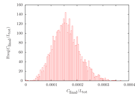
Figure 1: Frequency distribution of $C_{\rm final}/L_{\rm tot}$ for $4096$ independent realizations of Laskar’s model keeping fixed the total angular momentum of the system. In these calculations we fixed $L_{\rm tot}=2.2212\times 10^{-2}M_{\odot}\,{\rm AU}^{2}\,{\rm yr}^{-1}$, which is roughly the angular momentum of the planets of the Solar System.

To illustrate this point, in Fig. 1 we plot the frequency distribution of the final AMD normalised to the total angular momentum of the system, $C_{\rm final}/L_{\rm tot}$, for a large number of realizations of Laskar’s simplified model, keeping the total angular momentum of the system constant. The figure clearly illustrates the lack of constancy of the final AMD for different realizations. We further observe that $C_{\rm cr}$ can be defined as the supremum of $C_{\rm final}$; while this is a consistent definition, the numerical calculation of such quantity may be involved due to the poor statistics at the tail of the distribution.

Aside from the lack of conservation of $L_{\rm tot}$, in the numerical implementation of Laskar’s model, all relative orientations of the elliptic trajectories of the colliding particles that intersect lead to accretion with equal probability. In contrast, in the derivation of Eqs. 8 and 9, Laskar imposes a very specific collision among the particles. In either case, there is no physical constraint with respect to the relative velocity of the colliding particles, as stated by Safronov’s criterion (Safronov, 1972). The latter establishes that accretion is possible if the motion of the colliding particles satisfies $v_{\rm rel}\leq v_{\rm esc}$, where $v_{\rm rel}$ is the relative velocity of the colliding particles at the point of collision, and $v_{\rm esc}$ is the escape velocity of the local two-body problem. The former depends –among other parameters defining the elliptic orbits– on the relative orientation $\theta$, while the latter can be written as $v_{\rm esc}^{2}=2\mu/r_{H}$, where $r_{H}$ is the Hill radius defined with respect to the dominating mass. Moreover, the accretion probability in Laskar’s original model is independent of the orbital and physical parameters of the particles, being in this sense tantamount of an orderly type of growth (Wetherill & Stewart, 1989). While this is certainly a good starting point, it is intuitively important to include a mass-dependence in the accretion probability, since it affects the collision cross-section. A particular case of interest is the so-called runaway growth (Greenberg et al., 1978), during which the more massive bodies grow faster than the lighter ones.

3 Variations on Laskar’s model

In this section we describe the variations and the numerical results obtained by implementing some variations to Laskar’s simplified planetary model. These variations impose, firstly, the conservation of the total angular momentum of the system, and secondly, address the consequences of using mass-dependent accretion processes and velocity selection mechanisms, not considered previously (Laskar, 2000a, b), without leaving the overall simplicity in the formulation and implementation of the model.

3.1 General characteristics of the simulations

For the numerical results presented in this section, we consider that the mass of the host star is one solar mass ($M_{0}=1M_{\odot}$), which we shall use as the unit of mass. We shall also fix the astronomical unit (AU) as the unit of distance and the yr as the unit of time. In these units we have $\mu={\cal G}M_{0}=4\pi^{2}\,{\rm AU}^{3}\,{\rm yr}^{-2}\,M_{\odot}^{-1}$. In addition, we shall fix the total mass of the disc to $M_{\rm disc}=1.3413\times 10^{-3}M_{\odot}$ and the total angular momentum of the system to $L_{\rm tot}=2.2212\times 10^{-2}M_{\odot}\,{\rm AU}^{2}\,{\rm yr}^{-1}$. These values are roughly the current values of mass and total angular momentum of the planets in the Solar System, respectively. These parameters define the physical quantities of our simulations.

In order to define the initial conditions, we must specify the form of the initial linear mass-density distribution $\rho_{a}(a)$ (or equivalently the initial surface density $\rho_{a}(a)/a$) and the initial eccentricity distribution $\rho_{e}(e)$. These distributions and the extension of the disc are constrained by the total mass and the total angular momentum of the system. In the continuum limit, the total angular momentum of the system is written as

$$L_{\rm tot}=\int_{a_{\rm min}}^{a_{\rm max}}\int_{0}^{e_{\rm max}}\rho_{a}(a)\rho_{e}(e)\sqrt{\mu a(1-e^{2})}\,da\,de.$$ (10)

Assuming that $a_{\rm min}$ and $e_{\rm max}$ are given quantities, Eq. 10 can be used to define the maximal extension of the initial disc, $a_{\rm max}$ . Notice that Eq. 10 can be explicitly integrated for a homogeneous eccentricity density $\rho_{e}(e)=\zeta_{e}$ and a power-law linear mass-density distribution, $\rho_{a}(a)=\zeta_{a}a^{z_{a}}$ (Hernández-Mena, unpublished).

For a fair comparison with Laskar’s results (Laskar, 2000a), our simulations are initiated with a large number (typically 10000 bodies) of equal mass planetesimals, which is the most constraining case in terms of equivalence of the planetesimal location (Namouni, Luciani & Pellat, 1996); similar results are obtained for a larger initial number of planetesimals. We also considered the planetesimals on coplanar orbits, defining their initial semi-major axes and eccentricities from a homogenous linear mass-density distribution $\rho_{a}(a)=\zeta_{a}$ and a homogeneous eccentricity distribution $\rho_{e}(e)=\zeta_{e}$, respectively. Using $a_{\rm min}=0.1$ AU and $e_{\rm max}=0.3$ in Eq. 10 yields for the maximal extension of the disc $a_{\rm max}\cong 15.93$ AU. This value of $a_{\rm max}$ is smaller (by a factor 2) than the $30-35$ AU estimate for the outer edge of the original planetesimal disc of the Solar System, proposed by Levinson & Morbidelli (2003). However, this value is fully consistent with the range for the initial conditions used for the giant planets in the simulations of Tsiganis et al. (2005). The contributions of the massive disc ($30-50$ M_⊕) that these authors include beyond the orbits of the planets up to $30-35$ AU are excluded from the values $M_{\rm disc}$ and $L_{\rm tot}$. Notice that the outer disc has also a constant linear mass-density (Tsiganis et al., 2005). Finally, we emphasize that the use of Eq. 10 to define the maximal extension of the initial disc, $a_{\rm max}$, is yet another difference with respect to Laskar’s implementation.

It is also worth describing the implementation of the Brownian motion that accounts for the chaotic evolution of the averaged equations. Instead of implementing it in the space of eccentricities, we accomplished this by the exchange of angular momentum between a pair of arbitrary planetesimals. Denoting the initial angular momenta of the chosen planetesimals by $l_{1}$ and $l_{2}$ and the corresponding final ones as $l_{1}^{\prime}$ and $l_{2}^{\prime}$, we write $l_{1}^{\prime}=l_{1}+\delta l$ and $l_{2}^{\prime}=l_{2}-\delta l$. This ensures the conservation of the total angular momentum. The angular momentum exchanged is written as $\delta l=\beta\xi$. Here, $\beta\leq 1$ is a positive dimensionless parameter related to the diffusion constant; in our simulations we considered the value $\beta=10^{-3}$ which is small enough to model the slow secular chaotic diffusion (Laskar, 1989, 1990). The random walk character is provided by the stochastic variable $\xi$, which is a uniformly distributed random number in the interval $[-c_{2}^{\prime},c_{1}^{\prime}]$. Here, $c_{1}^{\prime}$ and $c_{2}^{\prime}$ are the largest positive numbers (with units of angular momentum) that simultaneously satisfy the inequalities $c_{1}^{\prime}\leq C_{1}$, $c_{1}^{\prime}\leq l_{2}$, $c_{2}^{\prime}\leq C_{2}$, $c_{2}^{\prime}\leq l_{1}$, where $C_{1}$ and $C_{2}$ are the AMD’s of the planetesimals. This definition of $\delta l$ ensures that both $l_{1}^{\prime}$ and $l_{2}^{\prime}$ lie in the correct intervals and the new eccentricities are well-defined. Note that this definition permits collisions of very eccentric ($e_{i}\sim 1$) planetesimals with the host star (Weidenschilling, 1975). This is consistently taken into account in our simulations whenever the perihelion of a particle is smaller than the radius of the Sun ($4.65\times 10^{-3}$ AU).

3.2 Laskar’s model including angular momentum conservation: orderly growth

We shall discuss firstly the case where we impose consistently the conservation of the total angular momentum within the simplified model of Laskar. This is aimed to clarify the differences that arise with the variations we implement with respect to Laskar’s results. As mentioned above, the simulations end once the system satisfies the AMD stability criterion. We carry out accretion and orbit evolution by selecting at random a planetesimal and one of its neighbours for accretion, and then proceed with the exchange of angular momentum between (many) pairs of planetesimals, also chosen at random. The mass distribution evolves smoothly, which makes this case similar to an orderly growth (cf. Armitage, 2010).

In Fig. 2 we present the final planetary configurations by combining the results of all $4096$ realizations of the model, plotting the mass and eccentricity of the formed planets in terms of their semi-major axis. Figure 3 illustrates the resulting final configuration of one planetary system taken at random from the set of realizations. In both figures (and throughout this section), the final planetary masses are given in units of the mass of Jupiter $M_{J}$ ($1M_{\odot}=1047.56M_{J}$; $1M_{J}=317.83M_{\oplus}$).

The results presented in Fig. 2(a) show an increasing trend of the planetary masses up to $a\approx 14.5$ AU, where a rapid decrease of $m$ in terms of $a$ takes place. The latter is due to the finite size of the planetesimal disc and the conservation of the angular momentum, and corresponds to the location of the outermost planet of the planetary systems formed. We observe that the largest planetary mass attained is $\sim 0.2M_{J}$, which is a comparatively small value with respect to the mass of Jupiter. This is a consequence of the large number of planets formed in each simulation, producing an average of $30.9\pm 1.7$ planets (the error is the standard deviation).

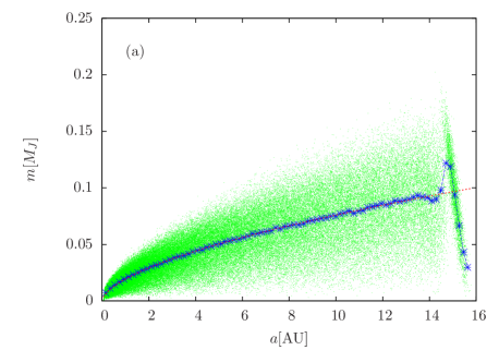
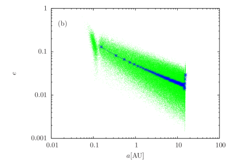
Figure 2: (a) Final planetary mass and (b) eccentricity in terms of the corresponding semi-major axis for $4096$ realizations of Laskar’s simplified model, imposing the conservation of the total angular momentum of the system. Each dot represents a planet formed in one of the simulations. The star symbols represent local averages taken over a semi-major axis interval of $0.2$ AU. In the top panel, the curve represents the power-law fit (Eq. 11) of the averaged data in the interval $a\in[0,14.5]$.

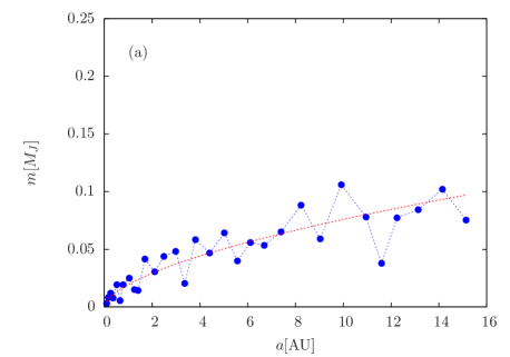
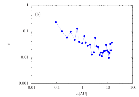
Figure 3: (a) Final planetary mass and (b) eccentricity in terms of the semi-major axis for a typical (randomly chosen) planetary system, obtained by implementing Laskar’s simplified model with conservation of the total angular momentum (orderly-growth model). The continuous curve in the top panel is the the power-law fit (Eq. 11) obtained from the averaged data of the ensemble of Fig. 2(a).

As illustrated in Fig. 3, individual planetary systems may not display the purely initial increasing behaviour of $m(a)$ observed in the data of the ensemble. The results of the ensemble are statistical and it is thus meaningful to define the average behaviour of the ensemble. Laskar (2000a) computes the average of the final planetary mass and semi-major axis for fixed planet number $n$. Since $n$ is not an observable quantity, we have opted to average the results over a small interval of the semi-major axis, which was fixed to $0.2$ AU. The resulting (binning) average is represented by the star symbols in Fig. 2. For comparison with Eq. 9, we fit the averaged data with the power-law function

$$m(a)=Aa^{\nu}.$$ (11)

According to Eq. 9 we should expect $\nu=1/2$. The continuous curve in Fig. 2(a) illustrates the resulting best-fitting, which in this case was calculated up to $a=14.5$ AU where the decreasing branch of the last planet sets in; the best-fitting yields $\nu\approx 0.59$. This value of $\nu$ is close but larger than Laskar’s predicted value $1/2$. We attribute this difference to the (implicit) dependence of the distribution of $C_{\rm cr}$ on the specific parameters of the model; this dependence is not considered in the integration of Eqs. 8 and 9. In Fig. 3(a) we also plot the best-fitting curve, in order to compare the results of a specific random planetary system with the results averaged over the ensemble.

Figure 2(b) displays the results of the final planetary eccentricity for the ensemble on a logarithmic scale, and Fig. 3(b) the corresponding results for a typical member of the ensemble. We observe a discontinuous behaviour around $a\sim 0.1$ AU. This feature is similar to the discontinuity related to the location of the outermost planet discussed in the mass diagram; in this case, it indicates the localisation of the innermost planets. The figure shows that the final eccentricities are smaller for larger semi-major axis (Jones, 2004). Planets with smaller masses display larger eccentricities in comparison with planets with larger masses. This is a consequence of the accretion processes, which tend to circularise the planetary orbits, consequently causing the more massive planets to exhibit smaller eccentricities than those less massive.

3.3 Mass-selection mechanism: runaway growth

As mentioned earlier, in Laskar’s original model the accretion probability is independent of the mass of the planetesimals. Yet, mass increases the collisional cross-section and thus promotes accretion, at least once the gravitational attraction among planetesimals starts to dominate their dynamics. We consider now the inclusion of such effects in the model. We address the case where the massive bodies grow quite fast due to their mass, and thus increase their difference in mass with respect to the lighter bodies. This happens until they exhaust the available mass in their surroundings. In what follows, we shall refer to this process as mass-selection or runaway growth (Greenberg et al., 1978; Wetherill & Stewart, 1989). Notice that, while we are including now the mass to select the particle that accretes, the relative velocity of the colliding particles is not yet taken into account, which is another important property that enhances gravitational focussing (Armitage, 2010).

We implement the mass-selection growth as follows. At each iteration of the model we define a threshold mass $m_{\rm cut}$, which is a uniformly-distributed random number between zero and the mass of the heaviest planetesimal. We then select at random a planetesimal whose mass is larger than this threshold mass, and implement the accretion process with one of its randomly-selected neighbours; the relative orientation of the elliptic orbits of the colliding particles is considered as before. With this simple implementation, once a particle has a mass slightly larger than the rest, i.e., from the first iteration, the probability that this particle is selected for collision in the next iteration is dramatically increased in comparison to other particles. This promotes accretion of the more massive particles, and hence mass growth in a runaway-like form. Additionally, it will systematically open a gap around the location of the accreted particle, since the distance to the nearest neighbours increases. Eventually, the nearest particles will be far enough to avoid collisions with this particle, i.e., the geometric condition 7 is not satisfied. In this case the planetesimal becomes locally isolated, until another particle is close enough again or enough angular momentum has been exchanged to allow for a new collision. If the particles that satisfy the condition $m_{i}>m_{\rm cut}$ can not collide with their neighbours (the isolation mass is locally reached), we then reset the value of $m_{\rm cut}$ to a smaller value, and proceed as described above. Clearly, this implementation promotes accretion of the more massive planetesimals. The chaotic diffusion following the accretion processes is implemented as before. Again, the simulations are iterated until the condition of AMD stability is reached.

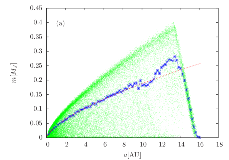
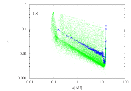
Figure 4: Same as Fig. 2 combining $4096$ realizations of the model, when the implementation includes runaway (mass-selection) growth. In the top panel, the fit with the power-law Eq. 11 of the averaged data, represented by the continuous curve, was carried in the interval $a\in[0,11.4]$.

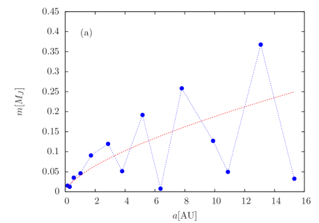
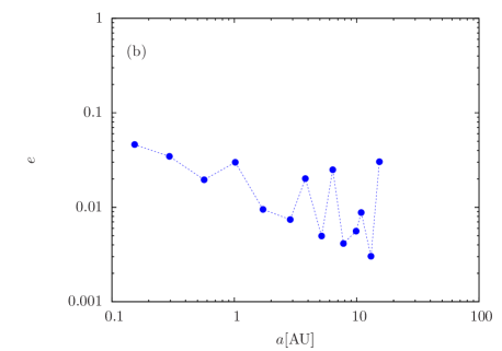
Figure 5: Same as Fig. 4 for one typical planetary system obtained in the runaway (mass-selection) growth model. The continuous curve in the top panel corresponds to the power-law fit of the averaged data in Fig. 4(a).

In Fig. 4 we present the results of the runaway (mass-selection) growth model, illustrating the combined results of the masses and eccentricities of the final planetary configurations in terms of their semi-major axes, for $4096$ independent realizations of the model. Figure 5 displays similar results for a single planetary system chosen at random. As illustrated by the results of the ensemble, the mass increases with the semi-major axis up to $a\approx 13.4$ AU, where a sudden decrease of the mass takes place. This is similar to the case of orderly growth, where the decreasing branch marks the location of the outermost planet formed. As done before, we fit the local averaged mass (up to $11.4$ AU) with the power-law function (Eq. 11). This yields the exponent $\nu\approx 0.66$, which is larger than the one obtained for the averaged data of Fig. 2(a). We have chosen to fit up to $a=11.4$ AU because, beyond this value, the averaged mass displays a strong oscillation. Notice that the overall mass-scale is enhanced by a factor close to $2$ with respect to the orderly-growth case, but the largest accreted particles are at most $0.4M_{J}$. The average final number of formed planets is reduced to $14.6\pm 1.15$.

It is interesting to compare the density of points in the mass–semi-major-axis diagram. For a given small interval of $a$, in Fig. 2(a) the density of the ensemble of planets is quite uniform with respect to the mass they reach (except towards the upper edge). This statement holds essentially for all $a$ before the last-planet branch appears. On the other hand, the density of points in Fig. 4(a) is manifestly non-uniform, at least for semi-major axis larger than $\sim 2$ AU. Indeed, considering a small interval of semi-major axis, there is a marked clustering of points towards the upper and lower edges of the mass. According to these observations, this runaway-growth mechanism yields larger final planetary masses, and thus a smaller number of planets, but also a systematic occurrence of small-mass planets for essentially all values of $a$. Since these planetary systems are AMD stable, these small-mass planets are far from planetary collisions. In this case, possible mean-motion resonances not included in the model could increase their eccentricities and eventually yield new collisions (see e.g. Laskar & Gastineau (2009)).

The eccentricities of the planetary ensemble obtained in this case, illustrated in Fig. 4(b), differ also from those resulting from orderly growth, cf. Fig. 2(b). Figure 4(b) shows the lack of uniformity in the density of points; yet, we note there is a density concentration towards comparatively smaller values of the eccentricity. That is, comparing the average value of the eccentricity for a given interval around $a$ for orderly and runaway growth, in the latter the average eccentricity is smaller, except for large values of $a$. Therefore, the mass-selection mechanism induces more circularised orbits of the planets, and in this sense, the final configurations are more stable. We also note that in the present case, individual planets typically with small $a$, may reach comparatively larger values of the eccentricity.

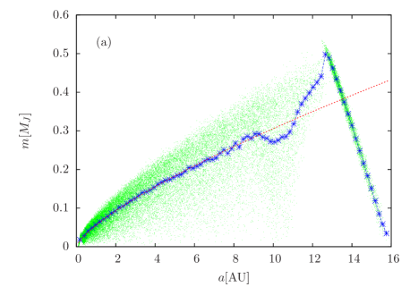
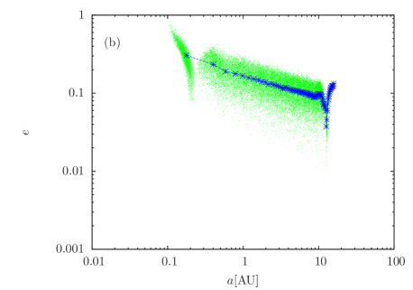
Figure 6: Same as Fig. 2 for the combined results of $4096$ simulations of the velocity-selection accretion model. In the top panel the continuos curve represents the fit of the power-law carried out in the interval $a\in[0,9.34]$.

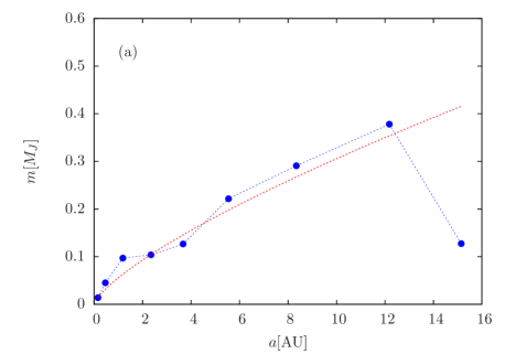
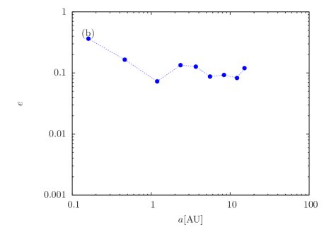
Figure 7: Same as Fig. 6 for a random planetary system obtained in the velocity-selection model. The continuous curve in the top panel is the power-law fit of the averaged data displayed in Fig. 6(a).

3.4 Velocity-selection mechanism

Another important factor that influences the accretion probability is the ratio between the relative velocity of the colliding bodies and their escape velocity. In particular, this quantity enters in the collisional cross-section through the gravitational focusing factor (Wetherill & Stewart, 1989)

$$F_{g}=1+v_{\rm esc}^{2}/v_{\rm rel}^{2}.$$ (12)

Here, $v_{\rm rel}$ is the relative velocity of the colliding particles (at infinity), and $v_{\rm esc}$ is the escape velocity in the local two-body problem. For $v_{\rm rel}/v_{\rm esc}\ll 1$ the gravitational factor enhances the collision cross-section. Moreover, in this case the colliding bodies are expected to be bound together and thus promote planetary growth (see Armitage, 2010).

One naive way of implementing these effects into Laskar’s simplified model with the conservation of angular momentum, is by selecting the relative orientation of the ellipses of the colliding bodies, such that the condition $v_{\rm rel}/v_{\rm esc}\ll 1$ is satisfied. That is, we allow accretion of particles only when Safronov’s condition is fulfilled. Carrying on these simulations resulted in systems where the AMD stability condition was not fulfilled, in general. Therefore, the elliptic trajectories of nearby bodies may intersect and thus collide, but for those collisions no value of $\theta$, the relative orientation of the ellipses, exists that $v_{\rm rel}/v_{\rm esc}\ll 1$ is fulfilled.

We therefore relaxed Safronov’s condition for accretion, and fixed $\theta$ as the relative orientation of the ellipses where $v_{\rm rel}$ achieves its minimum value. By doing this, we promote a moderate enhancement of the collisional cross-sections by the gravitational focussing factor, as well as quasi-tangential collisions. The latter is physically plausible for accretion (Ohtsuki, 1993). We note that with this implementation, the change in the absolute value of the energy after accretion is minimal, cf. Eq. 5, thus minimising the net migration of the accreted particle. We shall refer to this mechanism as the velocity-selection mechanism.

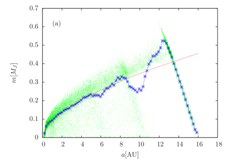
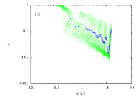
Figure 8: Same as Fig. 2 for the combined results of $4096$ simulations of the oligarchic growth model. In the top panel the continuos curve represents the fit of the power-law carried out in the interval $a\in[0,8.6]$.

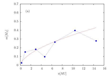
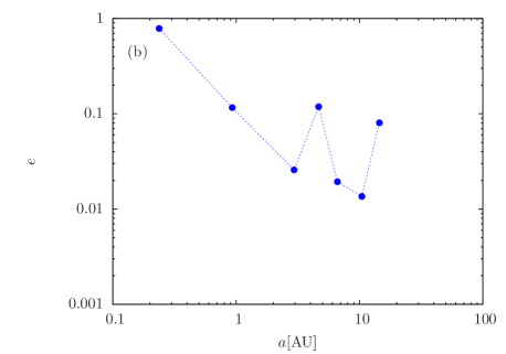
Figure 9: Same as Fig. 8 for a randomly selected planetary system obtained in the oligarchic growth model. The continuous curve in the top panel is the power-law fit of the averaged data displayed in Fig. 8(a).

The results of these simulations are shown in Fig. 6, for the combined results of the ensemble, and in Fig. 7 for an individual planetary system taken at random. As shown in the results for the ensemble, the mass increases with the semi-major axis up to $a\approx 12.6$ AU, where the feature associated with the location of the outermost planet appears. Fitting Eq. 11 with the local average mass up to $9.34$ AU yields the power-law exponent $\nu\approx 0.74$. This value of $\nu$ is even larger than the one obtained for runaway accretion. The mass-scale is larger as well, being enhanced by about $25\%$ with respect to the mass-selection mechanism; the maximum mass reaches approximately $0.53~{}M_{J}$. Correspondingly, the average final number of planets is further reduced to $9.3\pm 0.7$. As done before, the limit for fitting the power-law was considered due to the appearance of the strong oscillations in the averaged data, as illustrated in Fig. 6(a).

The density profile displayed in Fig. 6(a) resembles the one obtained for the orderly growth model, being more uniform than the density profile for runaway growth. Yet, there is a qualitative difference with respect to the former results, which is manifested by a gap in the mass–semi-major axis diagram. Indeed, there is a region in the $m$ vs $a$ diagram, defined beyond $10.7$ AU (for small masses), where no planet is formed. That is, planets formed beyond $\sim 10$ AU have a mass above a certain lower bound, which depends on $a$. Actually, a similar feature can also be observed for small values of $a$. We also note the less-massive planets formed at intermediate semi-major axis are consistently more massive than the corresponding ones for the mass-selection mechanism.

With respect to the eccentricities of the ensemble, as illustrated in Fig. 6(b), we confirm the overall resemblance with the results obtained for orderly growth, where $\theta$ is a uniformly-distributed random variable in the proper interval. In the present case, the distribution of final planetary eccentricities yields the possibility of larger values of the eccentricity. This can be noticed, e.g., in the branch of small $a$ associated with the location of the innermost planets, and for large values in the sudden increase of the average eccentricity of the outermost planets.

3.5 Mass- and velocity-selection mechanism: oligarchic growth

We consider now the combined effect of the mass- and velocity-selection mechanisms. To this end, we select a particle according to the mass-selection mechanism described previously, and then select the relative orientation $\theta$ of the elliptic orbits of the colliding particles such that $v_{\rm rel}$ is a minimum. This case is somewhat analogous to oligarchic growth models (Kokubo & Ida, 1998), where after an initial runaway phase, gravitational focussing is enhanced by all the dominating protoplanets but on a slower time-scale. We shall thus use this name to refer to the present case. The combined results of $4096$ simulations are shown in Fig. 8, and the result of one randomly selected realisation in Fig. 9.

As illustrated in Fig. 8(a), the results display an increasing behaviour of the mass upon the semi-major axis, until the feature associated with the position of the outermost planet appears. In this case, fitting the averaged data with Eq. 11 in the interval $a\in[0,8.6]$ yields $\nu\approx 0.58$. This value is comparable (marginally smaller) than the value obtained for orderly growth. Despite this, the overall mass-scale is slightly larger than in previous cases, reaching the value $0.63~{}M_{J}$, consequently yielding a smaller average number of formed planets: $6.9\pm 0.7$.

With regards to the final eccentricities, Fig. 8(b) illustrates the enhancement of the final eccentricity of the orbits. Indeed, we observe an increased variance of the final eccentricity at all scales of the semi-major axis, as well as their average value. In particular, we note that for the outermost planet, the corresponding eccentricity may reach values close to $0.2$. Interestingly, this indicates that the distribution of $C_{\rm final}$ has larger values than in the other cases.

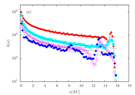
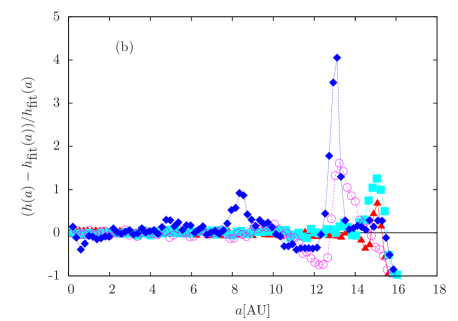
Figure 10: (a) Number of planets $h(a)$ formed in an interval of size $\Delta a\sim 0.2$ AU around $a$. The symbols identify the different growth models: Triangles (red) for orderly growth (Laskar’s model with conservation of $L_{\rm tot}$), squares (cyan) for runaway growth, empty circles (magenta) for the velocity-selection mechanism, and filled circles (blue) for oligarchic growth. The dashed lines are the best-fitting power-law $h_{\rm fit}(a)$ for each case. (b) Relative residuals with respect to $h_{\rm fit}(a)$. The peaks indicate a systematic enhancement of the formation of planets in certain specific locations.

The density profiles displayed in the mass and eccentricity diagrams are interesting and differ clearly in the structure from the other cases. Indeed, not only the location of the outermost and innermost planets is noticeable, but actually the location of other planets can be estimated from the darken clumps that appear in the figures. This can also be observed in the oscillations displayed by the averaged data, which, in comparison with the cases discussed before, are more prominent and appear even for smaller values of $a$.

We illustrate these observations in Fig. 10. In Fig. 10(a) we plot the number of final planets $h(a)$ (on a log scale) located in an interval of size $\Delta a\sim 0.2$ AU centred around a semi-major axis $a$, for the four different growth models discussed. The dashed curves are the best-fitting power-law corresponding to each data set, which we denote $h_{\rm fit}(a)$. In all growth models, we observe a clear excess of particles (with respect to the best-fitting) towards the outer edge of the planetary systems, which is associated with the location of the outermost planet. The excess in the particle number with respect to $h_{\rm fit}(a)$ is close to or above $600$ particles in the orderly ($a\sim 15.1$ AU) and oligarchic ($a\sim 13.06$ AU) models, being more moderate in the other cases. We observe other peaks in the oligarchic growth model, at $a\sim 8.35$ AU and at $a\sim 4.8$ AU; in each case the excess of particles with respect to $h_{\rm fit}(a)$ becomes more moderate as the semi-major axis decreases. These observations point out the existence of other specific locations where planets are formed preferentially in the oligarchic model, once the AMD stability criterion is satisfied.

In order to show that such locations are indeed a systematic property with full statistical meaning, in Fig. 10(b) we display the relative residuals $[h(a)-h_{\rm fit}(a)]/h_{\rm fit}(a)$ of the corresponding fit for the four growth models. The location of the outermost peak in all models is at least a $65\%$ off the best-fitting. Notice that the case of the oligarchic growth corresponds to a deviation over $\sim 400\%$ from the best-fitting. With regards to the secondary peaks observed in the oligarchic growth model, they are $\sim 90\%$ and $\sim 29\%$ in excess with respect to $h_{\rm fit}(a)$, in decreasing order of $a$, respectively. This shows that these peaks are due to systematic correlations in the data, i.e., a systematic formation of planets in specific locations in this oligarchic growth model; in other words, an enhancement of the probability to find planets at those specific locations.

Figure 10(b) shows, in addition, that the peak associated with the outermost planet, that lies at the smallest semi-major axis, corresponds to the oligarchic growth one. This shows that migration is promoted by the combined effect of mass and velocity-selection mechanisms, as in the oligarchic growth model. Taking as reference the orderly growth model and comparing the results for mass and velocity-selection mechanisms, we see that the effect is largely dominated by the the latter mechanism.

4 Universality

An important question in relation to the results presented in the previous section, is what happens if the important physical parameters $L_{\rm tot}$, $M_{\rm disc}$, and $M_{0}$ have different values. Put differently, how do the results depend upon the specific values of $L_{\rm tot}$, $M_{\rm disc}$ and $M_{0}$. Notice that different values of these physical parameters may affect the radial extension of the disc, cf. Eq. 10. In this section, we address this question and show that the results are universal. Here, by universality, we mean that the results of different parameters are statistically the same under properly defined scaled variables. Notice that this universality may not hold by changing other parameters of the model such as $e_{\rm max}$, $\rho_{a}(a)$ or $\beta$ (Hernández-Mena, unpublished). This question is clearly of central importance for a comparison with the observations of exo-solar planetary systems.

To this end, we shall define the length-scale

$$R_{\rm scale}=[L_{\rm tot}/M_{\rm disc}]^{2}/\mu,$$ (13)

which is defined only in terms of the dynamically invariant quantities of the underlying many-body Hamiltonian (Eqs. 1–2). We emphasize here that $\mu=GM_{0}$ includes the dependence on the mass of the host star $M_{0}$, and is not fixed to $4\pi^{2}$ unless $M_{0}=M_{\odot}$. The dimensionless scaled variables are thus given by

$$a^{\prime} = a/R_{\rm scale},$$ (14)

$$m^{\prime} = m/M_{\rm disc}.$$ (15)

According to these equations, the masses of the planets formed scale linearly with the mass of the disc, i.e., $M_{\rm disc}$ defines simply the overall mass scale of the simulations. In turn, the semi-major axes scale linearly with $M_{0}$, and quadratically with the ratio of the total angular momentum and the mass of the disc.

We compare now equivalent calculations for the same growth model using different physical parameters. We shall use the oligarchic growth model of Section 3.5 as example, and compare with calculations performed for the same values of $M_{0}$ and $M_{\rm disc}$, which therefore will not change the mass-scale of the formed planets, but with the total angular momentum of the system fixed to $L^{\prime}_{\rm tot}=3.479\times 10^{-2}M_{\odot}\,{\rm AU}^{2}\,{\rm yr}^{-1}$. The latter value is $\sim 1.57$ times the value used in Section 3.5.

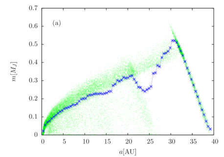
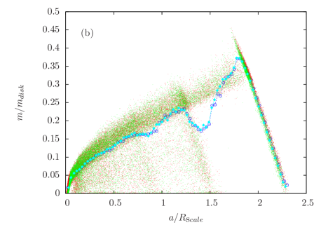
Figure 11: (a) Mass–semi-major axis diagram for the combined results of $4096$ simulations of the oligarchic growth model with total angular momentum of the system set to $L^{\prime}_{\rm tot}=3.479\times 10^{-2}M_{\odot}\,{\rm AU}^{2}\,{\rm yr}^{-1}$ ($M_{\rm disc}$ and $M_{0}$ are the same as in the simulations of Section 3.5). (b) Same as the top panel but using the scaled variables, Eq. 14 and 15, displaying the data used in (a) and the data used in Fig. 8(a).

Figure 11(a) shows the mass–semi-major axis diagram for this case. The figure is quite similar, in a qualitative sense, to Fig. 8(a). Quantitatively, the vertical scales of both figures coincide, as expected. The horizontal scale is enlarged by a factor close to $2.5$ (actually, $(L^{\prime}_{\rm tot}/L_{\rm tot})^{2}$). In Fig. 11(b) we display the same correlation diagram using the scaled variables defined in Eqs. 14 and 15, for the data of both parameter sets. The difficulty to distinguish the data from one case to the other clearly illustrates the meaning of universality. We emphasize that the same scaling holds for the position of the peaks of the relative residuals that mark the systematic formation of planets at certain specific locations. Equivalent results can be obtained by varying the values of $M_{\rm disc}$ and $M_{0}$.

The universal property illustrated in Fig. 11 is a consequence of the fact that the ($N+1$)-body Hamiltonian (Eqs. 1–2) includes only terms which build up a homogeneous potential (of degree -1), thus being invariant under appropriate scaling (Landau & Lifshitz, 1976). Therefore, universality actually holds for any dynamical variable and also for all the growth models discussed here. This property opens another perspective to statistically analyse the data of exo-solar planetary systems.

Yet, the scaling property of universality may break down if other parameters used in the model strongly influence the results of the simulations. Changing the functional form of $\rho_{a}(a)$ will change the scaling properties of the mass in terms of the semi-major axis, which can be inferred from the analytical results of Laskar (2000a), cf. Eq. 9. Another more subtle situation arises, for example, when a much larger value of $L^{\prime}_{\rm tot}$ is considered, keeping all other parameters fixed. In this case, the initial planetesimals disc will be more extended with respect to the parameter corresponding value $a_{\rm max}$, with the same functional form of the initial $\rho_{a}(a)$, thus making up a much fainter planetesimal disc due to normalization. If the density is not taken consistently, the value of $e_{\rm max}$ used may become important in the simulations, since some collisions of particles may not take place for $L^{\prime}_{\rm tot}$. Adjusting the number of particles at the beginning of the simulations yields universality again.

5 Summary and concluding remarks

In this paper, we have studied some physically-motivated variations on Laskar’s simple model of accretion and evolution (Laskar, 2000a, b), simulating the formation and dynamics of planetary systems in the secular limit, thus excluding effects of mean-motion resonances. Fulfilling the AMD stability criterion ensures that planetary collisions are no longer possible for the averaged system, but might be possible if mean-motion resonances were included. The variations we incorporated include important situations which are relevant to the formation of planetary systems according to the current understanding (Safronov, 1972; Polack et al., 1996; Armitage, 2010). In particular, we implemented the model with a strict conservation of the total angular momentum of the system during the simulations. We also addressed the implications that arise from including in the accretion probability distribution a dependence on the mass of the planetesimals, and on the relative velocity of the colliding particles at the collision point. These are important factors that influence the accretion rate processes. In our implementation of these physical effects we have tried to maintain the simplicity of Laskar’s original model. An important limitation of our models, inherited from Laskar’s simplified model, is the lack of a true dynamical evolution, which thus prevents us from answering questions involving or addressing the physical time in the formation processes.

Our statistical analysis was based on the mass–semi-major axis correlations of the formed systems, using the current values of the total angular momentum and mass of the planets of the Solar System as main parameters, though we included also remarks on the final eccentricities. For the comparisons, we consider as reference Laskar’s model imposing the conservation of the total angular momentum of the system, which we referred to as orderly growth. This case shows a power-law behaviour of the mass of the formed planets in terms of the semi-major axes in accordance to Laskar’s prediction, but with a different value of the exponent. At the edges of the disc, our statistical results showed distinctive features deviating from this power-law behaviour, which are associated with the location of the inner- and outer-most planets. Introducing a mass-selection mechanisms where more massive bodies have an enhanced probability to accrete, thus modelling a kin of runaway growth, we found a comparatively smaller number of planets formed, which are more massive. Interestingly, we observed a systematic occurrence of rather small-mass remnants embedded in the planetary system. We also considered a velocity-selection mechanism by only allowing accretion when Safronov’s condition is satisfied; in this case, our results showed that the AMD stability criterion was not fulfilled in general. We thus relaxed this condition, and fixed the relative orientation of the elliptic orbits of the colliding bodies to the value corresponding to the minimum of the relative velocity. This criterion selects the quasi-tangential collisions, which take longer times of interaction, making physically plausible accretion. In this case, we found that the average number of planets was further reduced, which are then more massive, at the end of the simulations. Furthermore, the results manifest the appearance of a gap in the mass–semi-major axis diagram, which defines a lower bound for the masses of the planets at either edge, that depends on their location.

We also considered the combination of the mass- and velocity-selection mechanisms, in what we called the oligarchic growth model. In this case, the number of final planets was further reduced and their masses increased, with the peak reaching values over $0.6M_{J}$. An interesting result is the systematic appearance of planets at specific locations, manifested as a definite excess of planets formed in this growth model. This property is manifested as a clustering of planets, i.e., an enhancement in the density profile in definite regions of the mass–semi-major axis diagram. We emphasize that, despite the stochastic nature of the model, the combined mass- and velocity-selection mechanisms induce strong correlations that yield this clustering. We observed from the location of the outermost planet, that the strongest migration occurs precisely in this oligarchic growth, due fundamentally to the velocity-selection mechanism, i.e., gravitational focusing.

We also addressed the question of variations to the main physical parameters of the model. We found that the results are statistically invariant with respect to such changes, whenever they are expressed in terms of appropriate scaled variables. The masses scale linearly with the mass of the disc, and the semi-major axes scale according to Eqs. 13 and 14, involving the angular momentum, the mass of the disc and the mass of the central star. In this sense, the results are universal. Universality holds in particular when the same functional form of the initial distributions $\rho_{a}(a)$ and $\rho_{e}(e)$ are maintained. This property follows from the mechanical similarity of the Hamiltonian (Landau & Lifshitz, 1976).

In most of our simulations, we used the parameters describing the current state of the Solar System, and an initial homogeneous linear mass-density distribution $\rho_{a}(a)$. We expect that changing the initial linear mass-density distribution influences the power-law behaviour obtained, essentially as it does in the analytical results of Laskar (2000a). Comparing the masses of the planets formed in the simulations with those of the Solar System, in our simulations the inner planets are more massive, and the outer planets are thus not massive enough. Yet, it is interesting to remark that the occurrence of the specific locations (semi-major axes) where the planets form, obtained for the oligarchic growth model, are consistent with the initial conditions used for three (out of four) of the major planets considered in the simulations of the architecture of the Solar System performed within the first Nice model by Tsiganis et al. (2005); as mentioned, this unexpected agreement does not hold for the masses (Thommes, Duncan & Levison, 2003). Considering that our results are qualitative, such a partial quantitative agreement is encouraging to construct more realistic models, that fully explain the initial conditions of the Nice model in a statistical robust sense.

Future work along these lines will be aimed to incorporate in the model effects related to mean-motion resonances (Malhotra, 1995), which are known to be important in the architecture of the Solar System (Tsiganis et al., 2005; Morbidelli et al., 2007, 2009). Furthermore, improving on the assumed form of the initial linear mass-density distribution $\rho_{a}(a)$ may yield better comparison of the mass distributions. For the concrete case of the Solar System, Laskar (1997, 2000a) suggested that a better modelling may be an initial linear mass-density distribution that considers separately the inner and outer solar systems. Other possibilities include the distinction of particles as gas or heavy elements, or the addition of an outer planetesimal disc, as assumed by the Nice model.

References

- Armitage (2010) Armitage P.J., 2010, Astrophysics of Planet Formation, Cambridge University Press, Cambridge
- Batygin & Brown (2010) Batygin K., Brown M.E., 2010, ApJ 716, 1323
- Box & Draper (1987) Box, G.E.P., Draper, N.R., 1987, Empirical Model-Building and Response Surfaces, Wiley Series in Probability and Statistics, John Wiley & Sons, New York, pp. 424
- Fernández & Ip (1984) Fernández J., Ip W., 1984, Icarus 58, 109
- Greenberg et al. (1978) Greenberg R., Wacker J.F., Hartmann W.K., Chapman C.R., 1978, Icarus 35, 1
- Hernández-Mena (unpublished) Hernández-Mena C., PhD thesis, UAEM, unpublished
- Jones (2004) Jones H.R.A., 2004, in Holt S.S., Deming D., eds, AIP Conference Proceedings Vol 713, The Search for Other Worlds, American Institute of Physics, New York, pp. 17
- Kokubo & Ida (1998) Kokubo E., Ida, S., 1998, Icarus 131, 171
- Landau & Lifshitz (1976) Landau, L.D., Lifshitz, E.M., 1976, Mechanics, Course of theoretical physics vol 1, 3 ed., Butterworth-Heinemann, Oxford
- Laskar (1989) Laskar J., 1989, Nat 338, 237
- Laskar (1990) Laskar J., 1990, Icarus 88, 266
- Laskar (1997) Laskar J., 1997, A&A 317, L75
- Laskar (2000a) Laskar J., 2000a, Phys. Rev. Lett. 84, 3240
- Laskar (2000b) Laskar J., 2000b, ”AMD-stability and the organization of planetary systems”, preprint.
- Laskar & Gastineau (2009) Laskar J., Gastineau M., 2009, Nat 459, 817
- Levinson & Morbidelli (2003) Levison H. F., Morbidelli A., 2003, Nat 426, 419
- Malhotra (1995) Malhotra R., 1995, AJ 110, 420
- Morbidelli et al. (2007) Morbidelli A., Tsiganis K., Crida A., Levison H., Gomes R. 2007, AJ 134, 1790
- Morbidelli et al. (2009) Morbidelli A., Bresser R., Tsiganis K., Gomes R., Levinson H.L., 2009, A&A 507, 1041
- Namouni, Luciani & Pellat (1996) Namouni F., Luciani J.F., Pellat R., 1996, A & A 307, 972
- Nieto (1972) Nieto M.M., 1972, The Titius-Bode Law of Planetary Distances: Its History and Theory, Pergamon Press, Oxford
- Ohtsuki (1993) Ohtsuki K., 1993, Icarus 106, 228
- Polack et al. (1996) Pollack J.B., Hubickyj O., Bodenheimer P., Lissauer J.J., 1996, Icarus 164, 62
- Safronov (1972) Safronov V. S., 1972, Evolution of the ProtopIanetary Cloud and Formation of the Earth and Planets. NASA TTF-677, Israel Program for Scientific Translations, Keter Publishing House, Jerusalem
- Thommes, Duncan & Levison (2003) Thommes E. W., Duncan M. J., Levison H. F., 2003, Icarus, 161, 431
- Tsiganis et al. (2005) Tsiganis K., Gomes R., Morbidelli A., Levinson H.F., 2005, Nat 435, 459
- Weidenschilling (1975) Weidenschilling S.J., 1975, AJ 80, 145
- Wetherill & Stewart (1989) Wetherill G.W., Stewart G.R., 1989, Icarus 77, 330