Counts-in-Cylinders in the Sloan Digital Sky Survey with Comparisons to N-body Simulations

Abstract

Environmental statistics provide a necessary means of comparing the properties of galaxies in different environments and a vital test of models of galaxy formation within the prevailing, hierarchical cosmological model. We explore counts-in-cylinders, a common statistic defined as the number of companions of a particular galaxy found within a given projected radius and redshift interval. Galaxy distributions with the same two-point correlation functions do not necessarily have the same companion count distributions. We use this statistic to examine the environments of galaxies in the Sloan Digital Sky Survey, Data Release 4. We also make preliminary comparisons to four models for the spatial distributions of galaxies, based on $N$-body simulations, and data from SDSS DR4 to study the utility of the counts-in-cylinders statistic. There is a very large scatter between the number of companions a galaxy has and the mass of its parent dark matter halo and the halo occupation, limiting the utility of this statistic for certain kinds of environmental studies. We also show that prevalent, empirical models of galaxy clustering that match observed two- and three-point clustering statistics well fail to reproduce some aspects of the observed distribution of counts-in-cylinders on 1, 3 and 6-${\rm h}^{-1}{\rm Mpc}$ scales. All models that we explore underpredict the fraction of galaxies with few or no companions in 3 and 6-${\rm h}^{-1}{\rm Mpc}$ cylinders. Roughly $7\%$ of galaxies in the real universe are significantly more isolated within a 6 ${\rm h}^{-1}{\rm Mpc}$ cylinder than the galaxies in any of the models we use. Simple, phenomenological models that map galaxies to dark matter halos fail to reproduce high-order clustering statistics in low-density environments.

1. Introduction

Measurements of galaxy environments provide a crucial test of large-scale structure and of the physics of galaxy formation. Long used as a test of cosmological models (e.g., Blumenthal et al., 1984; Bryan & Norman, 1998; Bullock et al., 2002; Berlind et al., 2005; Berrier et al., 2006; Blanton & Berlind, 2007), environmental statistics become more powerful probes of galaxy formation models as the cosmological parameters of our Universe are measured with higher accuracy.

In the modern view of galaxy formation, galaxies form within dark matter halos. At any given epoch the relationship between galaxies and their dark matter halos can be described by a “halo occupation distribution” (HOD), which specifies the probability that a halo of mass $M$ hosts $N$ galaxies with a given criteria. This relationship is still quite difficult to predict from first principles, and thus it is useful to use measurements of various environmental statistics to empirically constrain this distribution and to inform more physical models. The two-point correlation function has long been among the most powerful tools to characterize large-scale structure, (e.g., Peebles, 1973; Kirshner et al., 1979; Davis & Peebles, 1983; de Lapparent et al., 1988; Norberg et al., 2001; Zehavi et al., 2005; Padmanabhan et al., 2007), and has frequently been used to constrain the HOD for a given galaxy population (Scoccimarro et al., 2001; Berlind & Weinberg, 2002; Abazajian et al., 2005; Lee et al., 2006; Zheng & Weinberg, 2007).

A related way to probe the distribution of galaxy environments is the close-pair fraction, which has been used widely in observational surveys to characterize the evolution of galaxy merger rates, enabling tests of the hierarchical merger sequence predicted by the standard cosmological model (Zepf & Koo, 1989; Yee & Ellingson, 1995; Patton et al., 1997, 2002; Lin et al., 2004; De Propris et al., 2005, 2007). Berrier et al. (2006) examined the evolution of the close-pair fraction of dark matter halos in an $N$-body simulation. They find that the close-pair fraction of dark matter halos does not directly measure the merger rate of galaxies. However, the predicted halo close-pair counts do match the observed close-pair fraction of galaxies, assuming that every sufficiently large dark matter halo contains a galaxy. While these results are encouraging, tests in other regimes are necessary to assess both the underlying cosmological model and the manner in which galaxies are related to overdensities of dark matter.

The local number density of galaxies has a well-established connection to the morphologies and colors of individual galaxies; this relationship is known as the morphology-density relation (Oemler, 1974; Dressler, 1980; Postman & Geller, 1984; Park et al., 2007). There are several methods of measuring density. Dressler (1980) uses the 10 nearest neighbors to calculate the local surface density. More recently, many groups use counts within spheres (Hogg et al., 2003; Blanton et al., 2003a, 2005a) or cylinders (Hogg et al., 2004; Blanton et al., 2006; Kauffmann et al., 2004; Barton et al., 2007) of fixed radius. As with group finding algorithms, this method suffers from both incompleteness and contamination. However, it is more straightforward and well-defined to implement number counts than a group-finding algorithm.

In this paper, we further explore the utility of counts-in-cylinders statistics as a diagnostic of galaxy formation models. We consider both semi-analytic galaxy formation models (based on publicly-available catalogs from the Millennium simulation) as well as methods based on halo abundance matching. The latter type of model uses high resolution dissipationless, cold dark matter simulations, combined with simple prescriptions for the galaxy–halo connection. Such models have proved remarkably successful in matching several statistics of the galaxy distribution, including two-point and three-point correlation functions (Carlberg, 1991; Colin et al., 1997; Kravtsov et al., 2004; Neyrinck et al., 2004; Conroy et al., 2006; Marín et al., 2008).

The paper is organized as follows. § 2 provides an overview of our analysis of counts-in-cylinders in the Sloan Digital Sky Survey data. In § 3 we discuss the $N$-body simulations and the phenomenological models used in our analysis. We compare the observational and simulation results as described in § 4. We give our primary results in § 5. First, we demonstrate the complementarity between the two-point correlation function and counts-in-cylinders statistics. We then use the counts-in-cylinders statistic to probe galaxy environments in several models for the galaxy distribution. Second, we show that galaxies in the SDSS sample are considerably more isolated than galaxies in any of four mock galaxy catalogs that we consider.

In § 6, we discuss our results and explore potential systematic issues stemming from either our simulation analysis or our treatment of the SDSS sample. We draw conclusions from our analysis in § 7.

2. Observational Data: the Sloan Digital Sky Survey

We use the Sloan Digital Sky Survey (SDSS), Data Release 4 (Adelman-McCarthy et al., 2006). Specifically, we use the Large Scale Structure subset of the NYU-Value Added Galaxy Catalog (NYU-VAGC), compiled by Blanton et al. (2005b). The combined spectroscopic sample in the NYU-VAGC covers an area of 2627 square degrees, to an apparent magnitude limit of $r=17.77$. Here we use the NYU-VAGC to create a volume-limited catalog of 27959 objects, limited to M${}_{\rm r}<-19+5\log{h}$, with redshift limits 0.0044 $\geq z\leq$ 0.0618.

Of course, the SDSS is an incomplete redshift survey. Fiber collisions cause an estimated incompleteness of $\sim$ 6%, all from pairs of galaxies closer than 55^′′ (Blanton et al., 2003c). An additional $\sim$ 1% of galaxies are missed because of bright foreground stars. As described below, we use the random catalogs provided on the NYU-VAGC website, which have the same geometry as the survey, to estimate the fraction of companions missed because of incompleteness, which we apply as a correction to the cylinder counts data. We also use the random catalogs to determine where the cylinder used for our companion counts analysis falls off the edge of the survey.

3. Simulations

We compare the SDSS data against several models for the galaxy distribution, based on $N$-body simulations. We use two different simulations, and for each simulation we examine two distinct methods for matching galaxies to dark matter host halos and subhalos; thus, we examine four distinct model galaxy catalogs, which we will refer to by their brief names (Z05 $V_{\rm in}$, Z05 $V_{\rm now}$, Millennium, and MPAGalaxies) as a convenient shorthand. Each of these models is physically motivated, though some are more strongly favored. We use them to test different physical models and to account for the cosmic variance we expect to find in an SDSS-sized sample. The simulations, models, and redshift surveys used in this paper are summarized in Table 1. Please note that the term “halos” is used throughout this work to mean “all halos” (i.e., both host and subhalos).

Table 1 Summary of Data and Simulations

Name	Type	Size ($({\rm h}^{-1}{\rm Mpc})^{3}$)	Description	Reason Included
SDSS DR4	Redshift Survey	3.034$\times 10^{6}$;	Observational data,	Data
		4783 square degrees	incompleteness $\sim$6%
Z05 $V_{\rm now}$	DM N-body+Semi-analytic Substructure	$(120)^{3}$	Model using current subhalo $V_{\rm max}$ as	Reduced resolution issues
			proxy for mass to assign luminosities
Z05 $V_{\rm in}$	DM N-body+Semi-analytic Substructure	$(120)^{3}$	Model using accreted subhalo $V_{\rm max}$ as	Reduced resolution issues
			proxy for mass to assign luminosities
Millennium	DM N-body Simulation	$(500)^{3}$	Use mass to assign luminosities	Large simulation used to calculate
				cosmic variance and check for
				systematic errors in $V_{\rm now}$
MPAGalaxies	Millennium + Semi-analytic	$(500)^{3}$	Use luminosities generated by model	Used to explore how more complicated
	Galaxy Modeling			galaxy assignment affects distribution

3.1. N-body Simulation and Substructure

The primary simulation to which we compare the data is a high resolution $N$-body simulation, previously described in Allgood et al. (2006), Wechsler et al. (2006), and Berrier et al. (2006). The simulations were performed using an Adaptive Refinement Tree (ART) $N$-body code (Kravtsov et al., 1997) with a cosmology of $\Omega_{m}$ = 0.3, $h$ = 0.7, and $\sigma_{8}$ = 0.9. The simulation consists of 512³ particles in a comoving box of 120 $h^{-1}$ Mpc on a side, with a particle mass of $m_{p}\simeq 1.07\times 10^{9}$ ${\rm h}^{-1}M_{\odot}$. This simulation is used to identify host halos, i.e., halos whose centers do not lie within the virial radius of larger halo. The host halos are complete down to virial masses of $M\simeq$ 10¹⁰ ${\rm h}^{-1}M_{\odot}$.

Substructure is included using the semi-analytic technique described in Zentner et al. (2005). As described in Berrier et al. (2006), we ignore substructure from the host halos, and replace it with substructure using the semi-analytic formalism. The number of subhalos that merge with a given host halo is determined using the extended Press-Schechter formalism (Somerville & Kolatt, 1999). Subsequently, we model the evolution of merged subhalos including both mass loss processes and dynamical friction. We track the evolution of the subhalos until their maximum circular velocities drop below $V_{\rm max}=80$ km $s^{-1}$. Adding this semi-analytic component to the simulation removes inherent resolution limits, eliminating the problem of “over-merging,” which is of particular importance for the enumeration of close pairs and companion counts we perform.

We use the maximum circular velocity of the halo, $V_{\rm max}$, as a proxy for luminosity in what follows, where $V_{\rm max}\equiv max[\sqrt{GM(<r)/r}]$. This measure is less ambiguous than any particular mass definition. Moreover, subhalos lose mass at their outskirts rapidly upon accretion, while halo interiors (and thus $V_{\rm max}$) are less severely affected by this mass loss, so this proxy is robust to mild mass loss that likely would not affect the galaxy that resides at the subhalo center. In this work, we use two distinct models to compare the simulation (which we will refer to as “Z05”) with observational data. The first model uses the $V_{\rm max}$ that the subhalo has at the epoch of interest (e.g., after it has been accreted by its host halo, evolved, and potentially lost significant mass). We will refer to this model as $V_{\rm now}$. Based on previous work (e.g., Conroy et al., 2006; Berrier et al., 2006), this model is not favored. However, we note the results for the sake of completeness, and for the sake of comparison to the Millennium simulation, which also reports the $V_{\rm max}$ at the epoch of interest (as described in § 3.3. The second model, the $V_{\rm in}$ model, assumes that luminosity is related to the $V_{\rm max}$ that the subhalo had just as it was being accreted and prior to dynamical evolution. The $V_{\rm in}$ model has been shown to reproduce the galaxy two-point correlation function at many epochs (Conroy et al., 2006), as well as the galaxy close-pair fraction (Berrier et al., 2006) very well. For subhalos $V_{\rm now}$ is smaller than $V_{\rm in}$, because $V_{\rm in}$ characterizes subhalos prior to the removal of mass by the interaction with the host halo. As a result, the $V_{\rm now}$ model has fewer subhalos above any fixed maximum velocity threshold. The average number of subhalos for a host of a given mass for each of these models is shown in Figure 1. These models are also described in more detail in Berrier et al. (2006).

3.2. Identifying Galaxies with Halos

To best compare the simulations to the data from SDSS, we treat the simulation output as if it were a redshift survey, by assigning luminosities to the dark matter halos and restricting the information used to that which would be obtainable from actual observations.

Since the N-body substructure simulations contain no model for luminous matter, we use the published $r$-band luminosity function from the SDSS (Blanton et al., 2003b), and assign luminosities to the subhalos to match the observed galaxy number densities. Following Kravtsov et al. (2004), Conroy et al. (2006) and Berrier et al. (2006), we assume a one-to-one relation between dark matter halos (including subhalos within larger host halos) and galaxies. Larger halos correspond to brighter galaxies. We establish this relation as follows: for any $r$-band magnitude, we integrate the luminosity function to compute the cumulative number density of observed galaxies brighter than this magnitude. We match this to a halo $V_{\rm max}$ by assigning this magnitude to the $V_{\rm max}$ value for which the cumulative number density of all halos is the same as the cumulative number density of observed galaxies.

For the Z05 simulation, we use both the $V_{\rm in}$ and $V_{\rm now}$ models. As discussed in Berrier et al. (2006), assigning luminosities based on the $V_{\rm now}$ model assumes that baryons may be stripped significantly from the galaxy as it evolves in the potential of the larger host, thus gradually reducing the galaxy luminosity. This model underproduces satellite galaxies in the simulation. Alternatively, using $V_{\rm in}$ to calculate the number density assumes that the baryons are more tightly bound than the dark matter, and that the luminous galaxy does not lose significant stellar mass after accretion onto the larger host. The true evolution is likely between these extremes. The $V_{\rm in}$ model has significant observational support, but we consider both models here for the purposes of comparison.

After the luminosities are assigned, we use all halos and subhalos with M${}_{\rm r}<-19+5\log{h}$ (which corresponds to $V_{\rm max}$ = 137 km $s^{-1}$ for the $V_{\rm in}$ model and $V_{\rm max}$ = 127 km $s^{-1}$ for $V_{\rm now}$). “Moving” the simulation out to a distance of 500 ${\rm h}^{-1}{\rm Mpc}$, to cover the appropriate redshift space, we convert the x, y, z coordinates to RA, Dec, and redshift. We then compute the distance on the sky in exactly the same way as we do for the redshift survey. We employ periodic boundary conditions with the simulations to ensure that the cylinder we are using never falls off the edge.

3.3. Millennium Simulation

The Millennium simulation was performed with the GADGET-2 code (Springel, 2005) and follows the evolution of 2160³ particles of mass $8.6\times 10^{8}$ ${\rm h}^{-1}M_{\odot}$ in a box 500 ${\rm h}^{-1}{\rm Mpc}$ on a side (Springel et al., 2005). The cosmology is comparable to that of the Z05 simulation. In particular, the Millennium simulation cosmology is spatially flat with $\Omega_{m}$ = 0.25, $h$ = 0.73, and $\sigma_{8}$ = 0.9. Halo identification was performed at run-time during the numerical simulation and the resultant halo catalogs, which we use in the present study, are publicly available. The stated completeness limit of these catalogs is $M\geq 1.7\times 10^{10}h^{-1}$ M_⊙. For our purposes, the primary advantage of the Millennium simulation, and the halo and galaxy catalogs produced from it, is the large volume compared with the Z05 models. The Millennium simulation volume is $\sim 42$ times larger than the volume-limited SDSS sample we consider.

The Millennium Database does not provide $V_{\rm max}$ for all subhalos, so we use halo mass as a proxy for galaxy luminosity in this case. We assign luminosities as described in § 3.2, where we rank simulated halos by their mass, observed galaxies by their $r$-band luminosities, and map halo mass onto luminosity by matching the cumulative number densities at the mass and luminosity thresholds. For field halos, this is much like the $V_{\rm now}$ model described above, aside from variations in $V_{\rm max}$ at fixed mass due to variations in the internal structures of halos. For subhalos, the relation between $V_{\rm max}$ and mass may be significantly altered and exhibit larger scatter due to the interactions between the satellite objects and the host potentials. We assign luminosities by the abundance matching method, rank ordering both halos and galaxies, so we expect that in broad terms this assignment should be similar to the $V_{\rm now}$ model in so much as there is little difference between rank ordering by mass or $V_{\rm max}$. We expect these assignments to be significantly different in the central regions of host halos, where the influence of interactions on subhalos is large.

For further comparison we also use the MPAGalaxies database described in De Lucia & Blaizot (2007). De Lucia & Blaizot (2007) use a semi-analytic technique to model the galaxies associated with the dark matter halos of the Millennium Simulation. De Lucia & Blaizot (2007) model the stellar components of these galaxies using the Bruzual & Charlot (2003) stellar population synthesis model, with the Chabrier (2003) IMF and Padova 1994 evolutionary tracks. Galaxy mergers follow the mergers of their host dark matter halos until the halos fall below the resolution limit of the simulation. At that point, De Lucia and Blaizot calculate the survival time of the galaxies using their orbits and the dynamical friction time. Mergers result in a “collisional starburst” modeled by the prescription in Somerville et al. (2001).

3.4. The Two-Point Correlation Function

As stated in § 1, for several, simple and well-motivated assignments of galaxy luminosity to dark matter halos, predicted two-point correlation functions match observations well, particularly on large scales ($\gtrsim$ Mpc). Figure 2 shows the two-point functions of the simulated galaxy catalogs we consider compared to the SDSS measurement of the galaxy two-point function by Zehavi et al. (2005). In broad terms, the $V_{\rm in}$ model corresponds most closely to the SDSS data over the entire range of scales, as expected from the previous results of Conroy et al. (2006). The $V_{\rm now}$ and Millennium DM models deviate at relatively small separations.

The discrepancy seen at small separations between the Millennium dark matter halos and the other mock galaxy samples may have several causes. Most likely, this reflects the fact that the relation between halo $V_{\rm max}$ and remaining bound mass is significantly altered in dense environments relative to the field. It is also possible that the simulation could suffer from numerical dissolution of small subhalos in dense environments. The MPAGalaxies sample is consistent with the SDSS result above r $\cong$ .3 ${\rm h}^{-1}{\rm Mpc}$.

4. The Counts-in-Cylinders Environment Statistic

4.1. General Description

The counts-in-cylinders statistic that we use is similar to the one used by Kauffmann et al. (2004) and Blanton et al. (2006). We look at every halo or galaxy in the catalog and count how many companions it has within a cylinder with a radius defined by a given transverse separation and a depth given by a specified line-of-sight velocity difference. We choose a cylinder depth that is large enough to include all physically-associated galaxies, except in the most massive clusters. Specifically, we calculate the counts-in-cylinders for each galaxy using four different radii — $R_{c}~{}$ = 0.5 ${\rm h}^{-1}{\rm Mpc}$, 1 ${\rm h}^{-1}{\rm Mpc}$, 3 ${\rm h}^{-1}{\rm Mpc}$, and 6 ${\rm h}^{-1}{\rm Mpc}$ — searching for companions with velocity differences of $|\Delta$V — $\leq$ 1000 km s^-1.

4.1.1 Correcting for Incompleteness in the SDSS Data

Using the same technique, we measure the counts-in-cylinders statistic for galaxies in our volume-limited SDSS NYU-VAGC sample. We search each galaxy for all companions within $R_{c}~{}$ and $\Delta$V. The tools of the NYU-VAGC allow us to estimate the completeness in this cylinder. Specifically, we search four of the random catalogs of galaxies evenly distributed throughout the survey footprint in the apparent magnitude range and separation on the sky. We weight each of the random galaxies by the completeness of the sector from the “lss$\_$geometry.dr4.fits FGOTMAIN” parameter and by estimating what is missing from the limiting magnitude of the sector and the luminosity function of the survey (Blanton et al., 2005b). After applying this weight, we add the number of weighted random galaxies and normalize by the area searched on the sky. We then use the random counts as a measure of the local completeness of the survey, normalizing it to the mode for the survey and dividing by the completeness to arrive at an estimate of the corrected counts for a particular galaxy. When constructing histograms of the counts-in-cylinders statistics, we weight each galaxy by the inverse of its corresponding completeness to account for missing central (searched) galaxies in the survey.

Our correction for incompleteness undercounts the effects of missed close pairs, which are significantly more likely than “random” to be coincident in redshift space. We test the effects of these pairs by constructing an artificial simulation in which we eliminate 80% of the close pairs that would appear closer than 55 arcseconds on the sky, as assigned by a redshift distribution that matches the data. The effect is not systematic except at low companion counts, but even there the magnitude of the effect averaged over ¡= 5 companions is $\lesssim 5\%,10\%$, and $12\%$ for the 1, 3, and 6 ${\rm h}^{-1}{\rm Mpc}$ scales, respectively.

4.2. Sample Variance

By subdividing the Millennium simulation volume, we estimate the expected sample variance among volumes of the size of the SDSS volume-limited sample or the Z05 simulation box to ensure that any discrepancy we see is larger than can be attributed to natural variations in large scale structure. We calculate the cylinder counts in 64 sub-volumes from the Millennium simulation. Each sub-volume was cubic with a side length of 125 ${\rm h}^{-1}{\rm Mpc}$ and had a volume comparable to our Z05 catalogs. The histograms in Figure 3 show the cylinder counts for four of these volumes for the $R_{c}~{}$ = 3 ${\rm h}^{-1}{\rm Mpc}$ cylinder (bottom), and the variation from the total Millennium distribution (top). The errors are 68% from the scatter within a bin. We do a similar calculation for SDSS-sized volumes within Millennium. Those results determine the errors on the figures which include SDSS data.

The smooth blue line overlaid in Figure 3 shows the cylinder counts result from the Z05 $V_{\rm now}$ model. We use $V_{\rm now}$ because, as mentioned in § 3.3, this is the model to which the Millennium simulation results should be most closely related. The $V_{\rm now}$ result falls for the most part within the error bars of the Millennium distribution, with a $\chi^{2}$/(degrees of freedom [dof]) value of 0.609. The slight disagreement at the peak may be the result of a non-trivial relation between mass and $V_{\rm now}$ in dense regions, an inherent shortcoming in the Z05 model, or numerical overmerging and halo incompleteness in dense environments in the Millennium simulation. The first of these options is expected on physical grounds and seems most likely. The results for the $R_{c}~{}$ = 1 and 6 ${\rm h}^{-1}{\rm Mpc}$ cylinders show similar trends.

4.3. Companions as a Function of Host Halo Mass and Halo Occupation

To explore the utility of the counts-in-cylinders statistic, we consider it as a potential proxy for the masses of the dark matter host halos in which the galaxies reside. Various studies use counts-in-cylinders to test the halo model and other environment predictors (e.g., Blanton et al. 2006). We use the $V_{\rm in}$ model to calculate the average number of companions per galaxy within a host halo mass bin. Figure 4 shows the result for $R_{c}~{}$ = 0.5, 1, 3 and 6 ${\rm h}^{-1}{\rm Mpc}$ cylinders. The error bars are one standard deviation from the distribution within the bin. The counts-in-cylinders statistic tracks mass and halo occupation, but the relationships are extremely noisy. The $R_{c}~{}$ = 0.5 ${\rm h}^{-1}{\rm Mpc}$ cylinder can potentially distinguish between $\sim$ 10¹² and $\sim$ 10¹⁴ $M_{\odot}$ halos. The $R_{c}~{}$ = 1 ${\rm h}^{-1}{\rm Mpc}$ cylinder distinguishes 10¹² $M_{\odot}$ from 10¹³ $M_{\odot}$ and 10¹⁴ $M_{\odot}$. The $R_{c}~{}$ = 3 and 6 ${\rm h}^{-1}{\rm Mpc}$ cylinders only distinguish between halos at the extremes of the mass distribution. None of the cylinders works well for masses below 10^12.5 $M_{\odot}$, although this scale will vary with the magnitude limit of the sample. For masses this small, the cylinders frequently include multiple small, physically-distinct groups and clusters, rather than solely the subhalos within one large host. For large companion numbers, the smaller cylinders are ineffective because they often do not encompass the entire group, which may have a virial radius of $\sim 1{\rm h}^{-1}{\rm Mpc}$. Ideally, one would tune the cylinder radius and depth to the halo sample of interest.

The trends in the 1 and 6 ${\rm h}^{-1}{\rm Mpc}$ scales may relate to the result of Blanton et al. (2006). Blanton et al. show that galaxy color depends much more strongly on the 1 ${\rm h}^{-1}{\rm Mpc}$ density, as measured by counts-in-cylinders, than it does on the 6 ${\rm h}^{-1}{\rm Mpc}$ surrounding density.

In Figure 5, we explore the relationship between the average number of companions in a given cylinder and the actual number of subhalos residing within the host (the halo occupation). The solid lines in the four panels represent the case where the number of companions is equal to the halo occupation. We see that using a cylinder of $R_{c}~{}$= 1.0${\rm h}^{-1}{\rm Mpc}$ gives us a very good estimate of the halo occupation for host halos with fewer than $\sim$40 subhalos, while a cylinder of $R_{c}~{}$= 3.0 ${\rm h}^{-1}{\rm Mpc}$ is reasonable for host halos with $\sim$65-85 subhalos.

4.4. The Complementarity of Cylinder Counts and $N$-point Statistics

The cylinder count statistic is related to the correlation function. However, there are important differences. The two-point correlation function describes the probability of finding companions within a spherical shell of a given radius from a galaxy, and the three-point correlation function does the same for three galaxies at fixed separations from each other, and so on for the other $N$-point correlators. The cylinder-counts distribution gives the probability of finding a certain number of companions within a cylinder of a set radius from a given galaxy. While the average number of companions at the scale $R_{c}~{}$ is set by the integral of the two-point correlation function over the volume of the cylinder, the distribution of companion counts is not specified by the two-point function. For example, the variance of the companion counts depends upon the three-point function, the skewness of companion counts depends upon the four-point function, and so on. In principle, the distribution of companion counts is sensitive to all of the $N$-point correlators and can be an efficient way to access information not available through two- and three-point statistics (or through the mean of the companion counts) without undertaking the challenging task of computing higher-point correlation functions.

To illustrate the utility of cylinder-count statistics as a complement to the correlation function, we identify two distributions of galaxies that effectively yield the same two-point function, but have systematically different companion number distributions. As an example, we create a simple, toy galaxy distribution by modifying the Z05 $V_{\rm in}$ catalog. We rearrange the substructure so that host halos that contain at least one subhalo with 27-37 companions are stripped of all of their subhalo companions within a 3 ${\rm h}^{-1}{\rm Mpc}$ cylinder (leaving the total mass unchanged). These subhalos are then reassigned to a location within 1 ${\rm h}^{-1}{\rm Mpc}$ of a host halo with ¿37 companions. While this exercise has no explicit physical justification, it does create a test catalog where halos preferentially avoid environments with roughly $\sim 30-40$ companions.

The left-hand panel of Figure 6 shows the two-point correlation function of our toy catalog compared with the best fit line from SDSS referenced earlier and the two-point correlation function from the Z05 $V_{\rm in}$ model. The test catalog correlation function falls well within the error bars of the $V_{\rm in}$ correlation function.

In contrast, the right-hand panel of Figure 6 is the histogram of the number of companions within an $R_{c}~{}$ = 3 ${\rm h}^{-1}{\rm Mpc}$ cylinder for the test catalog, the $V_{\rm in}$ model and SDSS. The figure shows that the effects of the substructure reassignment. There is a noticeable dip in the test catalog data right around the mean, although the mean itself does not change significantly. Thus, the cylinder counts statistic yields different information about the distribution of substructure on the scale of the cylinder.

Notably, this tool gives more direct information about the distribution of substructure rather than the physical separation between objects. It complements the 2-point correlation function as a tool for determining the accuracy of clustering in simulations when compared to redshift surveys.

5. Results

5.1. Comparing the Models to the SDSS

We now use the cylinder counts distribution described above to compare the predictions from the simulation catalogs to the SDSS. We calculate 1-$\sigma$ uncertainties from the cosmic variance between SDSS-sized volumes within the Millennium Simulation to set the error bars for the SDSS data, and use the 1-$\sigma$ uncertainties from the cosmic variance between Z05-sized volumes as the error bars for the Z05 $V_{\rm in}$ and $V_{\rm now}$ distributions. We summarize our results in tables 2 and  3.

Figure 7 shows the counts-in-cylinders distribution for the $R_{c}~{}$ = 1 ${\rm h}^{-1}{\rm Mpc}$ cylinder on the left, and the cumulative fraction of galaxies or halos with fewer than the given number of companions on the right. The arrows denote the mean number of companions for each model.

We can use the $\chi^{2}$ statistic computed as a summation over the companion counts obtained in each model to assess the ability of each model to match the SDSS data. All values quoted are $\chi^{2}$/(dof), where the degrees of freedom (dof) equal the number of bins in the distribution. For the purposes of the $\chi^{2}$ calculation, all bins have a width of one companion (note that this does not correspond to the binning in Figures 7, 8, and  9). We ignore the correlation between different counts in computing $\chi^{2}$ and treat this statistic only as guidance. We find that the Z05 $V_{\rm now}$ model produces a $\chi^{2}/$(dof) value of 1.002. This is surprising, as previous studies (such as Conroy et al. (2006)) find that $V_{\rm in}$ tends to be the type of model that best matches two- and three-point clustering statistics. In this case, the Z05 $V_{\rm in}$ model has a $\chi^{2}$/(dof) value of 131.264, while the Millennium and MPAGalaxies distributions have $\chi^{2}$/(dof) = 1201.758 and 21.721, respectively. If we disregard the tail of the distributions, and look only at the bins with more than 0 but fewer than 10 companions, we find that the Z05 $V_{\rm in}$ value drops to 1.819, while $V_{\rm now}$ is 0.297, implying that the Z05 models are more consistent with the SDSS distribution at the peak. The Millennium and MPAGalaxies models are not significantly improved by such excisions and have a $\chi^{2}$/(dof) value ¿ 1 for all cylinder radii and subsamples. The cumulative fraction of galaxies with less than or equal to a given number of companions tells a similar story.

For the sake of clarity, we do not include the Millennium and MPAGalaxies samples in the remaining figures. We do, however, quote their $\chi^{2}$/(dof) values and companion fractions in Tables 2 and  3.

The 3 ${\rm h}^{-1}{\rm Mpc}$ cylinder produces a more problematic distribution, as seen in Figure 8. While the general shapes of the Z05 distributions look similar to the SDSS result, note that the first bin is is very low for both the models. The $\chi^{2}$/(dof) values for $V_{\rm in}$ and $V_{\rm now}$ in this case are 6.008 and 0.683, respectively. However, if we look only at the peak (¡ 50 companions), $\chi^{2}$/(dof) for $V_{\rm in}$ = 0.494 and $\chi^{2}$/(dof) for $V_{\rm now}$ = 7.379, favoring the $V_{\rm in}$ model. On the right hand side of the figure the discrepancy in the first bin is plainly demonstrated. While 1.7 $\%$ of the galaxies in the SDSS data have 1 or 0 companions, the simulations have a frequency of less than half that.

It is interesting to note that the means of the SDSS and simulation distributions appear to be consistent with each other (the greatest difference from the average of the means is 7.12, while the standard deviation of the means from the Z05-sized volumes is 7.24), while the counts-in-cylinders statistics are not. The agreement of the means may be expected from the agreement in the correlation function. This result is another illustration of the complementarity of the information contained in the full distribution of companion counts compared to either the correlation function or the mean companion count.

The results for the $R_{c}~{}$ = 6 ${\rm h}^{-1}{\rm Mpc}$ cylinder are shown in Figure 9. The underprediction by the simulations of galaxies with few companions is more pronounced at 6 ${\rm h}^{-1}{\rm Mpc}$, extending to galaxies with up to 20 companions. The $\chi^{2}$/(dof) values in this case for the whole distribution are 1.047 for $V_{\rm in}$ and 0.514 for $V_{\rm now}$.

Disregarding the first bin brings the Z05 values to $\chi^{2}$/(dof) = 0.944 for $V_{\rm in}$ and 0.401 for $V_{\rm now}$. Looking at just the peak (20 ¡ Number of Companions ¡ 110), we get 0.337 and 1.050 for $V_{\rm in}$ and $V_{\rm now}$, respectively. On the other hand, if we look only at galaxies with fewer than 20 companions, we find $\chi^{2}$/(dof) = 3.292 and 3.800 for $V_{\rm in}$ and $V_{\rm now}$. Again, the Z05 distributions are more consistent with the SDSS results at the peak than at low densities.

Table 2 Results of the $\chi^{2}$ analysis

$R_{c}~{}({\rm h}^{-1}{\rm Mpc})$	Z05 $V_{\rm in}$	Z05 $V_{\rm now}$	Millennium DM	MPAGalaxies
$R_{c}~{}$ = 1
Full	$\chi^{2}$/(dof) = 131.264	$\chi^{2}$/(dof) = 1.002	$\chi^{2}$/(dof) = 1201.758	$\chi^{2}$/(dof) = 21.721
0 ¡ bin ¡ 10	$\chi^{2}$/(dof) = 1.819	$\chi^{2}$/(dof) = 0.297	$\chi^{2}$/(dof) = 4.629	$\chi^{2}$/(dof) = 4.149
$R_{c}~{}$ = 3
Full	$\chi^{2}$/(dof) = 6.008	$\chi^{2}$/(dof) = 0.683	$\chi^{2}$/(dof) = 5.232	$\chi^{2}$/(dof) = 23.441
0 ¡ bin ¡ 50	$\chi^{2}$/(dof) = 0.494	$\chi^{2}$/(dof) = 7.379	$\chi^{2}$/(dof) = 3.011	$\chi^{2}$/(dof) = 2.604
$R_{c}~{}$ = 6
Full	$\chi^{2}$/(dof) = 1.198	$\chi^{2}$/(dof) = 0.514	$\chi^{2}$/(dof) = 3.675	$\chi^{2}$/(dof) = 4.349
20 ¡ bin ¡ 110	$\chi^{2}$/(dof) = 0.337	$\chi^{2}$/(dof) = 1.050	$\chi^{2}$/(dof) = 1.769	$\chi^{2}$/(dof) = 1.558

Table 3 Fraction of galaxies with fewer than given number of companions

Number of Companions	SDSS	Z05 $V_{\rm in}$	Z05 $V_{\rm now}$	Millennium DM	MPAGalaxies
$R_{c}~{}$ = 1 ${\rm h}^{-1}{\rm Mpc}$
¡= 1	0.352 $\pm$ 0.016 0.008	0.308 $\pm$ 0.006 0.004	0.360 $\pm$ 0.006 0.004	0.391	0.327
¡= 3	0.582 $\pm$ 0.018 0.010	0.497 $\pm$ 0.021 0.009	0.595 $\pm$ 0.021 0.009	0.664	0.530
¡= 5	0.715 $\pm$ 0.019 0.013	0.607 $\pm$ 0.034 0.016	0.726 $\pm$ 0.034 0.016	0.807	0.641
¡= 10	0.861 $\pm$ 0.021 0.016	0.744 $\pm$ 0.050 0.026	0.870 $\pm$ 0.050 0.026	0.941	0.777
$R_{c}~{}$ = 3 ${\rm h}^{-1}{\rm Mpc}$
¡= 1	0.017 $\pm$ 0.002 0.001	0.006 $\pm$ 0.003 0.001	0.005 $\pm$ 0.003 0.001	0.005	0.008
¡= 3	0.070 $\pm$ 0.006 0.005	0.036 $\pm$ 0.012 0.004	0.035 $\pm$ 0.012 0.004	0.035	0.045
¡= 10	0.310 $\pm$ 0.020 0.012	0.239 $\pm$ 0.025 0.013	0.258 $\pm$ 0.025 0.013	0.273	0.254
¡= 50	0.900 $\pm$ 0.024 0.018	0.786 $\pm$ 0.032 0.021	0.887 $\pm$ 0.032 0.021	0.943	0.776
$R_{c}~{}$ = 6 ${\rm h}^{-1}{\rm Mpc}$
¡= 2	0.002 $\pm$ 0.0004 0.0003	0.0003 $\pm$ 0.0002 0.0002	0.0001 $\pm$ 0.0002 0.0002	0.00007	0.0003
¡= 5	0.009 $\pm$ 0.0009 0.0008	0.002 $\pm$ 0.001 0.0006	0.001 $\pm$ 0.001 0.0005	0.001	0.004
¡= 50	0.485 $\pm$ 0.014 0.013	0.378 $\pm$ 0.023 0.013	0.416 $\pm$ 0.023 0.013	0.440	0.369
¡= 110	0.872 $\pm$ 0.018 0.016	0.719 $\pm$ 0.027 0.016	0.819 $\pm$ 0.027 0.017	0.890	0.706

6. Discussion

The comparison shows a mismatch between the galaxy assignment in the simulations and the SDSS data, when we look at the entire distribution. Here we test the robustness of the result to simple changes in the galaxy assignment scheme, and also investigate possible observational effects. § 6.1, § 6.2, and § 6.3 detail our results.

6.1. Color Modeling

One possible reason that the simulations do not match the SDSS data at large ($R_{c}~{}$ = 6 ${\rm h}^{-1}{\rm Mpc}$) scales is that we do not include any of the effects of varying mass-to-light ratios (M/L) in the models to which we assign luminosities (the Z05 models and the Millennium dark matter halos). It has been demonstrated that galaxy color is related to the environment, with galaxies in denser environments having redder colors and higher M/L (Balogh et al., 2004; Hogg et al., 2004; Tanaka et al., 2004; Weinmann et al., 2006; Poggianti et al., 2006; Martínez et al., 2006; Gerke et al., 2007). Here, we use the relationships from Weinmann et al. (2006), who relate the fraction of early, late, and intermediate galaxies to host dark matter halo mass, and Bell & de Jong (2001), who derive a color dependent M/L, where redder galaxies are dimmer for a given mass. To determine the effects of M/L on our statistic, we use the median color as a function of parent halo mass from Figure 11 of Weinmann et al. (2006) to assign a $g-r$ color to each subhalo. These colors were then used with the color-dependent M/L for SDSS bandpasses from Bell et al. (2003) to calculate an adjusted luminosity or an effective stellar mass. We then found a weighted number density from these adjusted luminosities, which was used to determine the actual luminosity from the SDSS luminosity function.

The color corrected Z05 $V_{\rm in}$ results for the 6 ${\rm h}^{-1}{\rm Mpc}$ cylinder are shown in the left panel of Figure 10. This analysis uses the largest possible contrast between late and early types, therefore causing the largest shift. While the shift in the distribution is in the correct direction (more galaxies with fewer companions), it only accounts for a small part of the difference between the simulation and observational data. The lack of simple color modeling is not the cause of this discrepancy. The mismatch of the MPAGalaxies sample, which does include color modeling, further supports this result.

6.2. Varying the $V_{\rm max}$ Cut

To further explore possible explanations for the mismatch in the distributions at large scales, we try two other models with the Z05 data. First, we vary the $V_{\rm in}$ model halos being detected near the $V_{\rm max}$ cutoff by decreasing the $V_{\rm max}$ cutoff by a random number between 0 and 25 km s^-1 for host halos, and increasing the $V_{\rm max}$ cutoff by a random number between 0 and 100 km s^-1 for subhalos before calculating the number density. This is a step away from the monotonic luminosity assignment that we have been using, and, by allowing more small host halos, might increase the fraction of isolated galaxies. The resulting distribution, shown in the right panel of Figure 10, falls in between the original $V_{\rm in}$ and $V_{\rm now}$ distributions. While it certainly changes the shape of the distribution, the $\chi^{2}$/(dof) value (3.292 for the full distribution) does not significantly improve on the original results, or increase the fraction of halos with ¡ 20 companions.

The right panel of Figure 10 also shows the distribution for a second model. Here we use the $V_{\rm in}$ velocities for subhalos in hosts with $V_{\rm max}$ ¡ $10^{13}$ $M_{\odot}$ and $V_{\rm now}$ for subhalos in hosts with $V_{\rm max}$ ¿= $10^{13}$ $M_{\odot}$. This procedure assumes that galaxies in large halos are more likely to be stripped of luminous matter than galaxies in small halos. This distribution results in a $\chi^{2}$/(dof) = 2.800. Once again, this does not correct the lack of isolated halos in the simulations.

6.3. Isolated Galaxies

The consistent feature in the cylinder counts distribution for all the of the models is the relative paucity of isolated galaxies compared to the observed frequency of isolated galaxies. To verify that this is not an artifact of the survey footprint, we examine a possible cause in our analysis of the SDSS data for the $R_{c}~{}$ = 6 ${\rm h}^{-1}{\rm Mpc}$ cylinder counts, where the effect is most pronounced. First, we check the images of the twenty-one galaxies in SDSS flagged as having no companions. We find that ten are within 6 ${\rm h}^{-1}{\rm Mpc}$ of an edge. While we do correct for edge effects in our analysis, we also recompute the fraction of isolated galaxies without those ten as a conservative estimate. Adopting the conservative estimate of eleven isolated galaxies in the SDSS distribution, we expect to find eighteen isolated halos in the $V_{\rm in}$ sample. We only find seven. Assuming Poisson statistics, the probability that we should find so few isolated galaxies in the $V_{\rm in}$ sample is $\approx 2\times 10^{-3}$ (this compares to $\sim 10^{-9}$ if all twenty one isolated galaxies are included). The probabilities for the other models are all lower by at least one order of magnitude. We conclude that the difference in isolated galaxy fraction is not caused by unaccounted for edge effects.

7. Conclusions

We have explored the counts-in-cylinders statistic, and used it to compare galaxy environments in the SDSS with environments measured in several models for the galaxy distribution based on dark matter simulations. We show that this statistic provides different information than the two-point function alone; it is possible for two catalogs to have similar two-point correlation functions, but companion distributions with very different shapes.

Our primary results are as follows.

1. There is a large scatter in the number of companions a dark matter halo of a given host mass or halo occupation has within a set cylinder. The counts-in-cylinders statistic is limited as a tool for determining the host halo mass of a galaxy.

2. We considered several models for assigning galaxies to the dark matter distribution, including models based on abundance matching to dark matter substructures as well a semi-analytic model from the Millennium simulation. Each of these models significantly underpredicts the number of galaxies with very few companions on $R_{c}~{}$ = 3 and 6 ${\rm h}^{-1}{\rm Mpc}$ scales.

3. While none of the simulations or models examined have a counts-in-cylinders distribution that is consistent with that of SDSS data, the two abundance matching models (Z05 $V_{\rm now}$ and $V_{\rm in}$) have similar distributions when the first few, very discrepant, bins (corresponding to the most isolated galaxies) are ignored.

4. The counts-in-cylinders test fails for models that match the two- and three-point correlation functions, highlighting its utility as a diagnostic.

We have tested the robustness of these results to a series of possible systematic errors. Simple changes to the color assignment or to the scatter model in the abundance matching approach do not change the conclusions. We have accounted for known effects in the completeness of the SDSS NYU-VAGC data. In addition, is its hard to see how any small scale incompleteness would explain the discrepancy seen on several Mpc scales.

Our results indicate that some observed galaxies in the real universe are significantly more isolated than any halos of comparable size. It does not appear that the discrepancy we have identified in the counts-in-cylinders can be easily resolved with a standard halo occupation approach that assumes that all of a galaxy’s properties are set by the mass of its host halo. In any case, this mismatch merits further study.

Figure 1.— Halo occupation distribution for the Z05 $V_{\rm in}$ and $V_{\rm now}$ models. The lines are the combined HODs for host halos and subhalos, while the points are the subhalos only. The $V_{\rm in}$ model allows more subhalos on average to survive in host halos of a given virial mass (where the virial overdensity $\Delta_{vir}$ $\simeq$ 337).

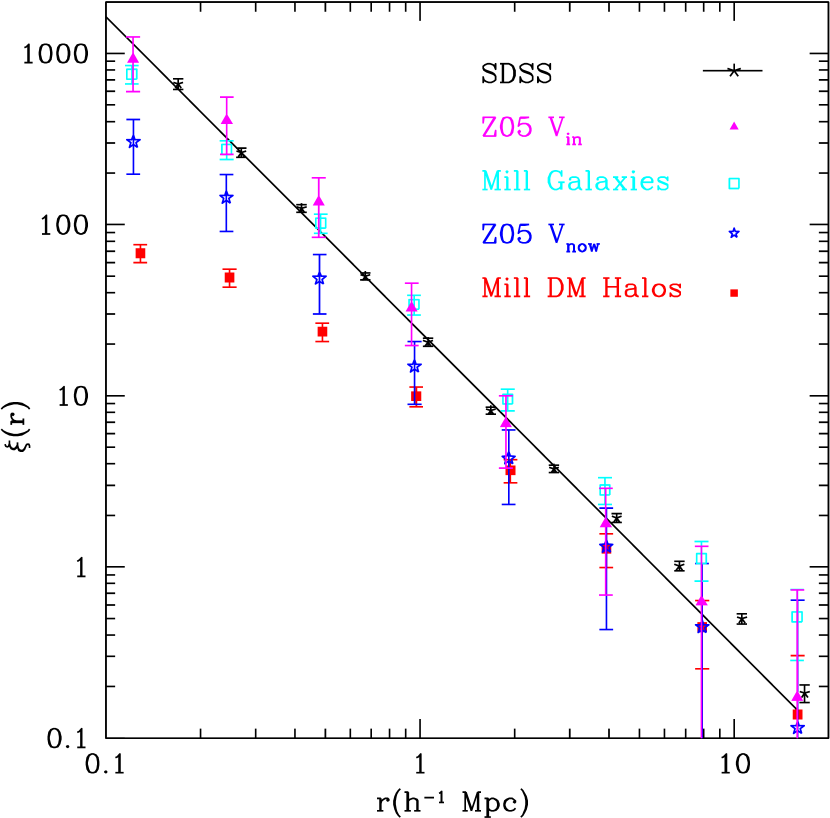
Figure 2.— Two-point correlation functions for models and data. The straight line is the power law fit to SDSS from Zehavi et al. (2005), $\xi(r)=(r/r_{0})^{-\gamma}$, with $r_{0}$ = 5.59 $\pm$ 0.11 ${\rm h}^{-1}{\rm Mpc}$ and $\gamma$ = 1.84 $\pm$ 0.01, while the black stars represent the actual data (I. Zehavi, private communication). The magenta triangles are the correlation function from the $V_{\rm in}$ model, the blue stars are from $V_{\rm now}$, the solid red squares are the Millennium simulation dark matter halos, and the open cyan squares are the Millennium simulation galaxies. The error bars are calculated by jackknifing over octants of the simulation for the Z05 models and over similarly sized subvolumes of the millenium sample.

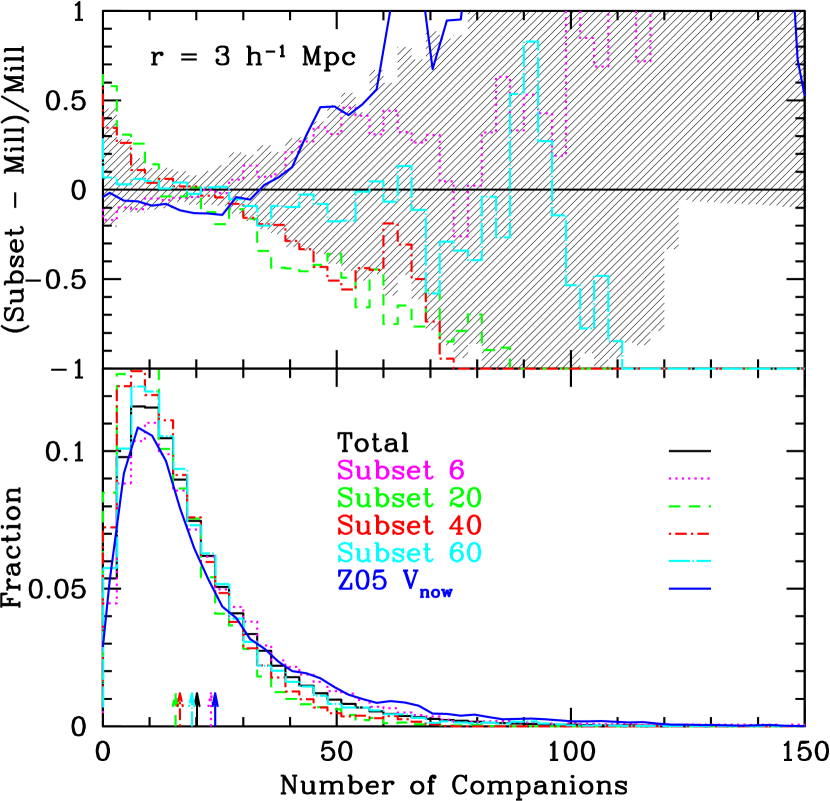
Figure 3.— Comparison of counts-in-cylinders between the Millennium simulation and the Z05 model (smooth blue line) for the 3 ${\rm h}^{-1}{\rm Mpc}$ cylinder. Bottom panel: Distribution of counts in $R_{c}~{}$ = 3 ${\rm h}^{-1}{\rm Mpc}$ cylinders. The arrows denote the mean of each distribution. Top panel: Fractional deviation from the mean cylinder counts. The shaded area denotes the dispersion among the $64$ sub-volumes of the Millennium simulation and provides a guideline for the statistical limitations of the comparison.

Figure 4.— Clockwise from top left: Average number of companions in the Z05 $V_{\rm in}$ sample within $R_{c}~{}$ = .5, 1, 6, and 3 ${\rm h}^{-1}{\rm Mpc}$ cylinders for galaxies within a given host halo mass bin. Shaded regions indicate the 1-$\sigma$ scatter in the value for each bin. Note that the y-axes have different scales.

Figure 5.— Clockwise from top left: Average number of companions in the Z05 $V_{\rm in}$ sample within $R_{c}~{}$ = .5, 1, 6, and 3 ${\rm h}^{-1}{\rm Mpc}$ cylinders for galaxies of a given halo occupation. Solid lines correspond to (halo occupation) = (number of companions) for comparison. Shaded regions indicate the 1-$\sigma$ scatter in the value for each bin.

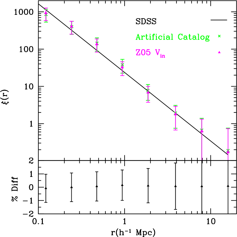
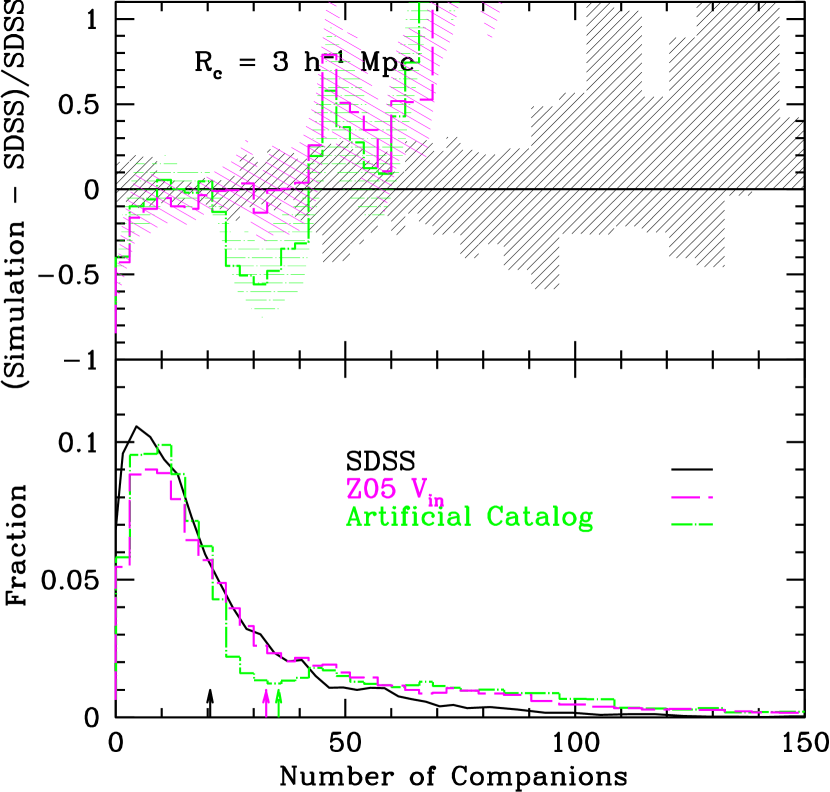
Figure 6.— Top left: Two-point correlation function for the artificial catalog (green “x”s) and the Z05 $V_{\rm in}$ model (magenta triangles) with the best fit line from SDSS. Error bars represent jackknife plus Poisson errors. Bottom left: the percent difference between the artificial catalog and the $V_{\rm in}$ model. Right: Histogram of the fraction of galaxies or halos with a given number of companions within an $R_{c}~{}$ = 3 ${\rm h}^{-1}{\rm Mpc}$ cylinder for the test catalog (green long-dash-short-dash line), the Z05 $V_{\rm in}$ data (magenta dashed line) and SDSS (black solid line).

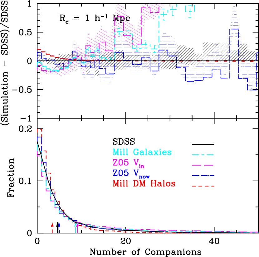
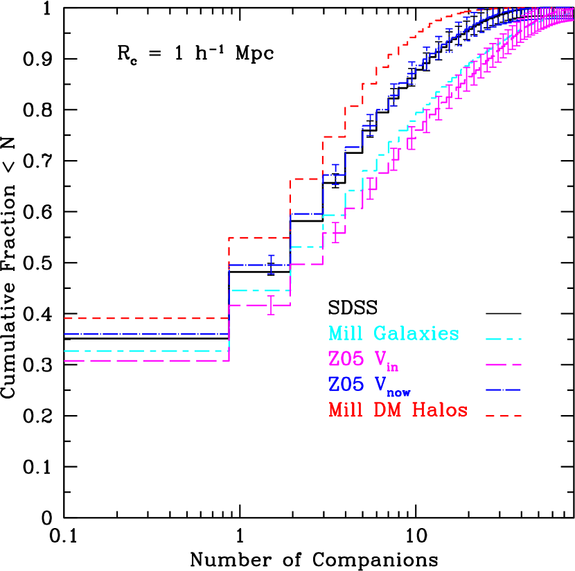
Figure 7.— Bottom left: Histogram of the fraction of galaxies or halos with a given number of companions within the $R_{c}$ = 1 ${\rm h}^{-1}{\rm Mpc}$ cylinder for Z05 $V_{\rm in}$ (magenta long-dashed line), $V_{\rm now}$ (blue dot-dashed line), Millennium (red short-dashed line), MPAGalaxies (cyan short-dashed-long dashed line), and SDSS (smooth solid black line). The arrows show the average number of companions for each distribution. Top left: Cylinders counts with the SDSS distribution subtracted. The shaded area is 1-$\sigma$ from cosmic variance between SDSS-sized volumes, while the error bars include the cosmic variance between Z05-sized volumes. Right: Cumulative fraction of of galaxies or halos with fewer than the given number of companions within the $R_{c}$ = 1 ${\rm h}^{-1}{\rm Mpc}$ cylinders.

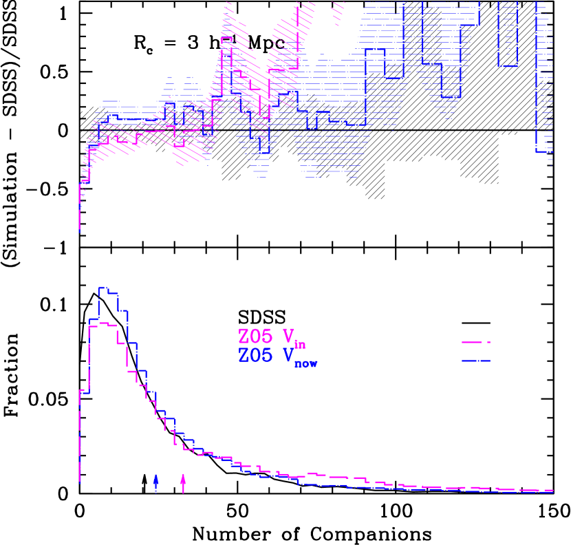
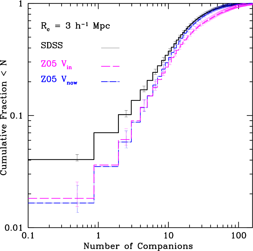
Figure 8.— Left: Cylinder counts for Z05 $V_{\rm in}$ (magenta long-dashed line), $V_{\rm now}$ (blue dot-dashed line), and SDSS (smooth solid black line) within $R_{c}~{}$ = 3 ${\rm h}^{-1}{\rm Mpc}$ cylinders. Right: Cumulative fraction of of galaxies or halos with fewer than the given number of companions within $R_{c}~{}$ = 3 ${\rm h}^{-1}{\rm Mpc}$ cylinders.

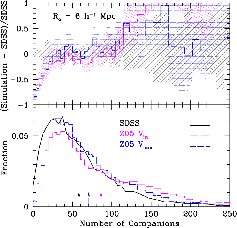
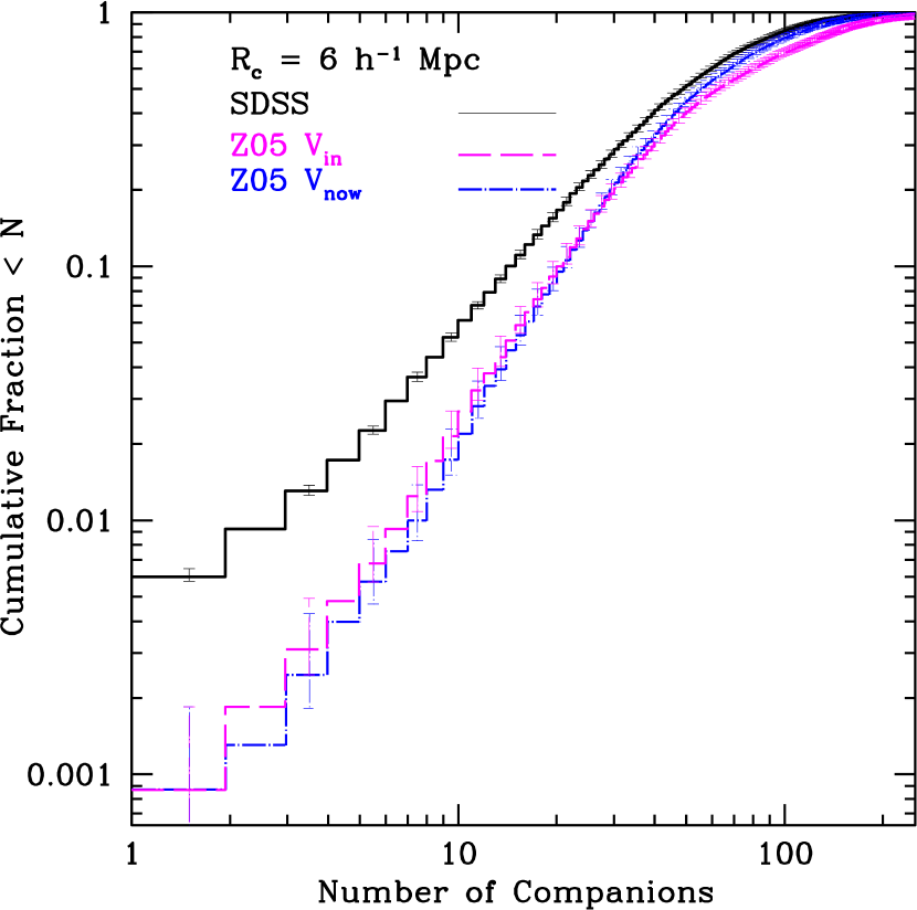
Figure 9.— Left: Cylinder counts for Z05 $V_{\rm in}$ (magenta long-dashed line), $V_{\rm now}$ (blue dot-dashed line), and SDSS (smooth solid black line) within $R_{c}~{}$ = 6 ${\rm h}^{-1}{\rm Mpc}$ cylinders. Right: Cumulative fraction of of galaxies or halos with fewer than the given number of companions within $R_{c}~{}$ = 6 ${\rm h}^{-1}{\rm Mpc}$ cylinders.

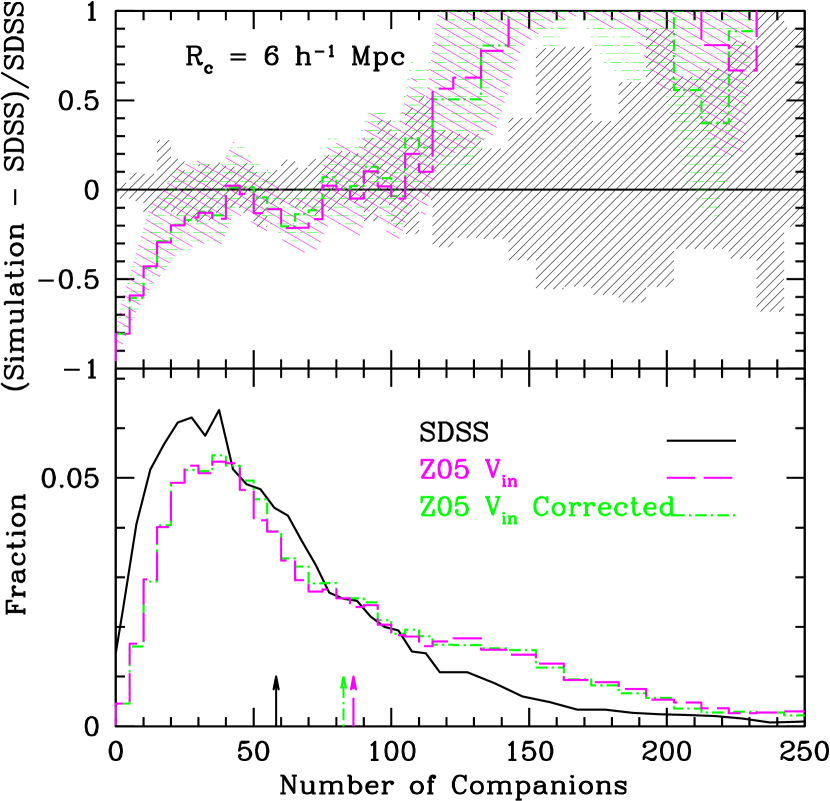
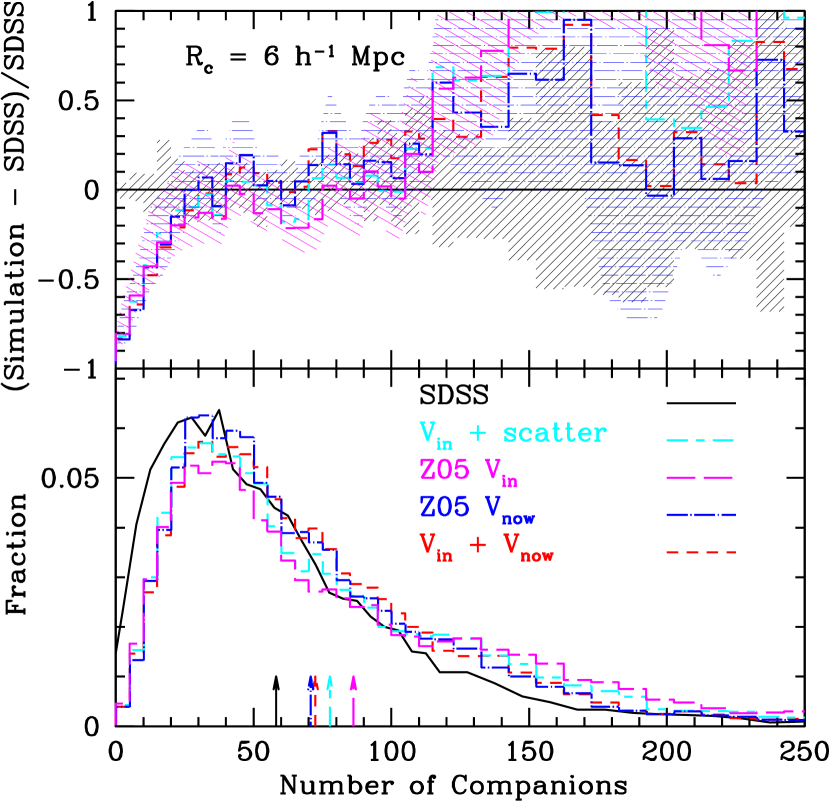
Figure 10.— Left: Cylinder counts for SDSS (smooth solid black line), Z05 $V_{\rm in}$ (magenta long-dashed line), and Z05 $V_{\rm in}$ with basic color correction (green short-dashed line) within 6 ${\rm h}^{-1}{\rm Mpc}$ cylinders. Right: Cylinder counts for SDSS (smooth solid black line), Z05 $V_{\rm in}$ (magenta long-dashed line), Z05 $V_{\rm now}$ (blue dot-dashed line), a combination of $V_{\rm in}$ and $V_{\rm now}$ (red short-dashed line), and $V_{\rm in}$ with scatter in the $V_{\rm max}$ cut ((cyan long-dashed–short-dashed line) within $R_{c}~{}$ = 6 ${\rm h}^{-1}{\rm Mpc}$ cylinders.

References

- Abazajian et al. (2005) Abazajian, K., Zheng, Z., Zehavi, I., Weinberg, D. H., Frieman, J. A., Berlind, A. A., Blanton, M. R., Bahcall, N. A., Brinkmann, J., Schneider, D. P., & Tegmark, M. 2005, ApJ, 625, 613
- Adelman-McCarthy et al. (2006) Adelman-McCarthy, J. K. et al 2006, ApJS, 162, 38
- Allgood et al. (2006) Allgood, B., Flores, R. A., Primack, J. R., Kravtsov, A. V., Wechsler, R. H., Faltenbacher, A., & Bullock, J. S. 2006, MNRAS, 367, 1781
- Balogh et al. (2004) Balogh, M. L., Baldry, I. K., Nichol, R., Miller, C., Bower, R., & Glazebrook, K. 2004, ApJ, 615, L101
- Barton et al. (2007) Barton, E. J., Arnold, J. A., Zentner, A. R., Bullock, J. S., & Wechsler, R. H. 2007, ApJ, 671, 1538
- Bell & de Jong (2001) Bell, E. F. & de Jong, R. S. 2001, ApJ, 550, 212
- Bell et al. (2003) Bell, E. F., McIntosh, D. H., Katz, N., & Weinberg, M. D. 2003, ApJS, 149, 289
- Berlind et al. (2005) Berlind, A. A., Blanton, M. R., Hogg, D. W., Weinberg, D. H., Davé, R., Eisenstein, D. J., & Katz, N. 2005, ApJ, 629, 625
- Berlind & Weinberg (2002) Berlind, A. A. & Weinberg, D. H. 2002, ApJ, 575, 587
- Berrier et al. (2006) Berrier, J. C., Bullock, J. S., Barton, E. J., Guenther, H. D., Zentner, A. R., & Wechsler, R. H. 2006, ApJ, 652, 56
- Blanton & Berlind (2007) Blanton, M. R. & Berlind, A. A. 2007, ApJ, 664, 791
- Blanton et al. (2005a) Blanton, M. R., Eisenstein, D., Hogg, D. W., Schlegel, D. J., & Brinkmann, J. 2005a, ApJ, 629, 143
- Blanton et al. (2006) Blanton, M. R., Eisenstein, D., Hogg, D. W., & Zehavi, I. 2006, ApJ, 645, 977
- Blanton et al. (2003a) Blanton, M. R., Hogg, D. W., Bahcall, N. A., Baldry, I. K., Brinkmann, J., Csabai, I., Eisenstein, D., Fukugita, M., Gunn, J. E., Ivezić, Ž., Lamb, D. Q., Lupton, R. H., Loveday, J., Munn, J. A., Nichol, R. C., Okamura, S., Schlegel, D. J., Shimasaku, K., Strauss, M. A., Vogeley, M. S., & Weinberg, D. H. 2003a, ApJ, 594, 186
- Blanton et al. (2003b) Blanton, M. R., Hogg, D. W., Bahcall, N. A., Brinkmann, J., Britton, M., Connolly, A. J., Csabai, I., Fukugita, M., Loveday, J., Meiksin, A., Munn, J. A., Nichol, R. C., Okamura, S., Quinn, T., Schneider, D. P., Shimasaku, K., Strauss, M. A., Tegmark, M., Vogeley, M. S., & Weinberg, D. H. 2003b, ApJ, 592, 819
- Blanton et al. (2003c) Blanton, M. R., Lin, H., Lupton, R. H., Maley, F. M., Young, N., Zehavi, I., & Loveday, J. 2003c, AJ, 125, 2276
- Blanton et al. (2005b) Blanton, M. R., Schlegel, D. J., Strauss, M. A., Brinkmann, J., Finkbeiner, D., Fukugita, M., Gunn, J. E., Hogg, D. W., Ivezić, Ž., Knapp, G. R., Lupton, R. H., Munn, J. A., Schneider, D. P., Tegmark, M., & Zehavi, I. 2005b, AJ, 129, 2562
- Blumenthal et al. (1984) Blumenthal, G. R., Faber, S. M., Primack, J. R., & Rees, M. J. 1984, Nature, 311, 517
- Bruzual & Charlot (2003) Bruzual, G. & Charlot, S. 2003, MNRAS, 344, 1000
- Bryan & Norman (1998) Bryan, G. L. & Norman, M. L. 1998, ApJ, 495, 80
- Bullock et al. (2002) Bullock, J. S., Wechsler, R. H., & Somerville, R. S. 2002, MNRAS, 329, 246
- Carlberg (1991) Carlberg, R. G. 1991, ApJ, 367, 385
- Chabrier (2003) Chabrier, G. 2003, PASP, 115, 763
- Colin et al. (1997) Colin, P., Carlberg, R. G., & Couchman, H. M. P. 1997, ApJ, 490, 1
- Conroy et al. (2006) Conroy, C., Wechsler, R. H., & Kravtsov, A. V. 2006, ApJ, 647, 201
- Davis & Peebles (1983) Davis, M. & Peebles, P. J. E. 1983, ApJ, 267, 465
- de Lapparent et al. (1988) de Lapparent, V., Geller, M. J., & Huchra, J. P. 1988, ApJ, 332, 44
- De Lucia & Blaizot (2007) De Lucia, G. & Blaizot, J. 2007, MNRAS, 375, 2
- De Propris et al. (2007) De Propris, R., Conselice, C. J., Driver, S. P., Liske, J., Patton, D., Graham, A., & Allen, P. 2007, ArXiv e-prints, 705
- De Propris et al. (2005) De Propris, R., Liske, J., Driver, S. P., Allen, P. D., & Cross, N. J. G. 2005, AJ, 130, 1516
- Dressler (1980) Dressler, A. 1980, ApJ, 236, 351
- Gerke et al. (2007) Gerke, B. F., Newman, J. A., Faber, S. M., Cooper, M. C., Croton, D. J., Davis, M., Willmer, C. N. A., Yan, R., Coil, A. L., Guhathakurta, P., Koo, D. C., & Weiner, B. J. 2007, MNRAS, 376, 1425
- Hogg et al. (2004) Hogg, D. W., Blanton, M. R., Brinchmann, J., Eisenstein, D. J., Schlegel, D. J., Gunn, J. E., McKay, T. A., Rix, H.-W., Bahcall, N. A., Brinkmann, J., & Meiksin, A. 2004, ApJ, 601, L29
- Hogg et al. (2003) Hogg, D. W., Blanton, M. R., Eisenstein, D. J., Gunn, J. E., Schlegel, D. J., Zehavi, I., Bahcall, N. A., Brinkmann, J., Csabai, I., Schneider, D. P., Weinberg, D. H., & York, D. G. 2003, ApJ, 585, L5
- Kauffmann et al. (2004) Kauffmann, G., White, S. D. M., Heckman, T. M., Ménard, B., Brinchmann, J., Charlot, S., Tremonti, C., & Brinkmann, J. 2004, MNRAS, 353, 713
- Kirshner et al. (1979) Kirshner, R. P., Oemler, Jr., A., & Schechter, P. L. 1979, AJ, 84, 951
- Kravtsov et al. (2004) Kravtsov, A. V., Berlind, A. A., Wechsler, R. H., Klypin, A. A., Gottlöber, S., Allgood, B., & Primack, J. R. 2004, ApJ, 609, 35
- Kravtsov et al. (1997) Kravtsov, A. V., Klypin, A. A., & Khokhlov, A. M. 1997, ApJS, 111, 73
- Lee et al. (2006) Lee, K.-S., Giavalisco, M., Gnedin, O. Y., Somerville, R. S., Ferguson, H. C., Dickinson, M., & Ouchi, M. 2006, ApJ, 642, 63
- Lin et al. (2004) Lin, L., Koo, D. C., Willmer, C. N. A., Patton, D. R., Conselice, C. J., Yan, R., Coil, A. L., Cooper, M. C., Davis, M., Faber, S. M., Gerke, B. F., Guhathakurta, P., & Newman, J. A. 2004, ApJ, 617, L9
- Marín et al. (2008) Marín, F. A., Wechsler, R. H., Frieman, J. A., & Nichol, R. C. 2008, ApJ, 672, 849
- Martínez et al. (2006) Martínez, H. J., O’Mill, A. L., & Lambas, D. G. 2006, MNRAS, 372, 253
- Neyrinck et al. (2004) Neyrinck, M. C., Hamilton, A. J. S., & Gnedin, N. Y. 2004, MNRAS, 348, 1
- Norberg et al. (2001) Norberg, P., Baugh, C. M., Hawkins, E., Maddox, S., Peacock, J. A., Cole, S., Frenk, C. S., Bland-Hawthorn, J., Bridges, T., Cannon, R., Colless, M., Collins, C., Couch, W., Dalton, G., De Propris, R., Driver, S. P., Efstathiou, G., Ellis, R. S., Glazebrook, K., Jackson, C., Lahav, O., Lewis, I., Lumsden, S., Madgwick, D., Peterson, B. A., Sutherland, W., & Taylor, K. 2001, MNRAS, 328, 64
- Oemler (1974) Oemler, A. J. 1974, ApJ, 194, 1
- Padmanabhan et al. (2007) Padmanabhan, N., Schlegel, D. J., Seljak, U., Makarov, A., Bahcall, N. A., Blanton, M. R., Brinkmann, J., Eisenstein, D. J., Finkbeiner, D. P., Gunn, J. E., Hogg, D. W., Ivezić, Ž., Knapp, G. R., Loveday, J., Lupton, R. H., Nichol, R. C., Schneider, D. P., Strauss, M. A., Tegmark, M., & York, D. G. 2007, MNRAS, 378, 852
- Park et al. (2007) Park, C., Choi, Y., Vogeley, M. S., Gott, J. R. I., & Blanton, M. R. 2007, ApJ, 658, 898
- Patton et al. (2002) Patton, D. R., Pritchet, C. J., Carlberg, R. G., Marzke, R. O., Yee, H. K. C., Hall, P. B., Lin, H., Morris, S. L., Sawicki, M., Shepherd, C. W., & Wirth, G. D. 2002, ApJ, 565, 208
- Patton et al. (1997) Patton, D. R., Pritchet, C. J., Yee, H. K. C., Ellingson, E., & Carlberg, R. G. 1997, ApJ, 475, 29
- Peebles (1973) Peebles, P. J. E. 1973, ApJ, 185, 413
- Poggianti et al. (2006) Poggianti, B. M., von der Linden, A., De Lucia, G., Desai, V., Simard, L., Halliday, C., Aragón-Salamanca, A., Bower, R., Varela, J., Best, P., Clowe, D. I., Dalcanton, J., Jablonka, P., Milvang-Jensen, B., Pello, R., Rudnick, G., Saglia, R., White, S. D. M., & Zaritsky, D. 2006, ApJ, 642, 188
- Postman & Geller (1984) Postman, M. & Geller, M. J. 1984, ApJ, 281, 95
- Scoccimarro et al. (2001) Scoccimarro, R., Sheth, R. K., Hui, L., & Jain, B. 2001, ApJ, 546, 20
- Somerville & Kolatt (1999) Somerville, R. S. & Kolatt, T. S. 1999, MNRAS, 305, 1
- Somerville et al. (2001) Somerville, R. S., Primack, J. R., & Faber, S. M. 2001, MNRAS, 320, 504
- Springel (2005) Springel, V. 2005, MNRAS, 364, 1105
- Springel et al. (2005) Springel, V., White, S. D. M., Jenkins, A., Frenk, C. S., Yoshida, N., Gao, L., Navarro, J., Thacker, R., Croton, D., Helly, J., Peacock, J. A., Cole, S., Thomas, P., Couchman, H., Evrard, A., Colberg, J., & Pearce, F. 2005, Nature, 435, 629
- Tanaka et al. (2004) Tanaka, M., Goto, T., Okamura, S., Shimasaku, K., & Brinkmann, J. 2004, AJ, 128, 2677
- Wechsler et al. (2006) Wechsler, R. H., Zentner, A. R., Bullock, J. S., Kravtsov, A. V., & Allgood, B. 2006, ApJ, 652, 71
- Weinmann et al. (2006) Weinmann, S. M., van den Bosch, F. C., Yang, X., & Mo, H. J. 2006, MNRAS, 366, 2
- Yee & Ellingson (1995) Yee, H. K. C. & Ellingson, E. 1995, ApJ, 445, 37
- Zehavi et al. (2005) Zehavi, I., Zheng, Z., Weinberg, D. H., Frieman, J. A., Berlind, A. A., Blanton, M. R., Scoccimarro, R., Sheth, R. K., Strauss, M. A., Kayo, I., Suto, Y., Fukugita, M., Nakamura, O., Bahcall, N. A., Brinkmann, J., Gunn, J. E., Hennessy, G. S., Ivezić, Ž., Knapp, G. R., Loveday, J., Meiksin, A., Schlegel, D. J., Schneider, D. P., Szapudi, I., Tegmark, M., Vogeley, M. S., & York, D. G. 2005, ApJ, 630, 1
- Zentner et al. (2005) Zentner, A. R., Berlind, A. A., Bullock, J. S., Kravtsov, A. V., & Wechsler, R. H. 2005, ApJ, 624, 505
- Zepf & Koo (1989) Zepf, S. E. & Koo, D. C. 1989, ApJ, 337, 34
- Zheng & Weinberg (2007) Zheng, Z. & Weinberg, D. H. 2007, ApJ, 659, 1