Numerical study of blow up and stability of solutions of generalized Kadomtsev-Petviashvili equations

Abstract.

We first review the known mathematical results concerning the KP type equations. Then we perform numerical simulations to analyze various qualitative properties of the equations : blow-up versus long time behavior, stability and instability of solitary waves.

1. Introduction

The main goal of this paper is an analysis of qualitative properties of solutions to generalized Kadomtsev-Petviashvili (KP) equations via a numerical approach.

The (classical) Kadomtsev-Petviashvili (KP) equations

(1) $$(u_{t}+u_{xxx}+uu_{x})_{x}\pm u_{yy}=0$$

were introduced in [57] to study the transverse stability of the solitary wave solution of the Korteweg- de Vries equation which reads in the context of water-waves

(2) $$u_{t}+u_{x}+uu_{x}+(\frac{1}{3}-T)u_{xxx}=0,\;x\in\mathbb{R},\;t\geq 0.$$

Here $T\geq 0$ is the Bond number which measures surface tension effects in the context of surface hydrodynamical waves.

Actually the (formal) analysis in [57] consists in looking for a weakly transverse perturbation of the one-dimensional transport equation

(3) $$u_{t}+u_{x}=0.$$

This perturbation, which is obtained by a Taylor expansion of the dispersion relation $\omega(k_{1},k_{2})=\sqrt{k_{1}^{2}+k_{2}^{2}}$ of the two-dimensional linear wave equation assuming $|k_{1}|\ll 1$ and $\frac{|k_{2}|}{|k_{1}|}\ll 1,$ amounts to adding a nonlocal term, leading to

(4) $$u_{t}+u_{x}+\frac{1}{2}\partial_{x}^{-1}u_{yy}=0.$$

Here the operator $\partial_{x}^{-1}$ is defined via Fourier transform,

$$\widehat{\partial_{x}^{-1}f}(\xi)=\frac{i}{\xi_{1}}\widehat{f}(\xi),\,\text{where}\;\xi=(\xi_{1},\xi_{2}).$$

Remark 1.

Equation (4) is reminiscent of the linear diffractive pulse equation

$$2u_{tx}=\Delta_{y}u,$$

where $\Delta_{y}$ is the Laplace operator in the transverse variable $y,$ studied in [8].

The same formal procedure is applied to the KdV equation (2), assuming that the transverse dispersive effects are of the same order as the x-dispersive and nonlinear terms, yielding the KP equation in the form

(5) $$u_{t}+u_{x}+uu_{x}+(\frac{1}{3}-T)u_{xxx}+\frac{1}{2}\partial_{x}^{-1}u_{yy}=0.$$

By change of frame and scaling, (5) reduces to (1) with the $+$ sign (KP II) when $T<\frac{1}{3}$ and the $-$ sign (KP I) when $T>\frac{1}{3}$.

Note however that $T>\frac{1}{3}$ corresponds to a layer of fluid of depth smaller than $0.46$ cm, and in this situation viscous effects due to the boundary layer at the bottom cannot be ignored. One could then say that “the KP I equation does not exist in the context of water waves”, but it appears naturally in other contexts (see for instance Remark 2 below).

Of course the same formal procedure could also be applied to any one-dimensional weakly nonlinear dispersive equation of the form

(6) $$u_{t}+u_{x}+f(u)_{x}-Lu_{x}=0,\;x\in\mathbb{R},\;t\geq 0,$$

where $f(u)$ is a smooth real-valued function (most of the time polynomial) and $L$ a linear operator taking into account the dispersion and defined in Fourier variable by

(7) $$\widehat{Lu)}(\xi)=p(\xi)\mathfrak{F}u(\xi),$$

where the symbol $p(\xi)$ is real-valued. The KdV equation corresponds for instance to $f(u)=\frac{1}{2}u^{2}$ and $p(\xi)=-\xi^{2}.$ Examples with a fifth order dispersion in $x$ are considered in [6], [58], [59].

This leads to a class of generalized KP equations

(8) $$u_{t}+u_{x}+f(u)_{x}-Lu_{x}+\frac{1}{2}\partial_{x}^{-1}u_{yy}=0,\;x\in\mathbb{R},\;t\geq 0.$$

Let us notice, at this point, that models alternative to KdV-type equations (6) are the equations of Benjamin–Bona–Mahony (BBM) type [10]

(9) $$u_{t}+u_{x}+uu_{x}+Lu_{t}=0$$

with corresponding two-dimensional “KP–BBM-type models” (in the case $p(\xi)\geq 0$)

(10) $$u_{t}+u_{x}+uu_{x}+Lu_{t}+\partial_{x}^{-1}\partial_{y}^{2}u=0$$

or, in the derivative form

(11) $$(u_{t}+u_{x}+uu_{x}+Lu_{t})_{x}+\partial_{y}^{2}u=0$$

and free evolution group

$$S(t)=e^{-t(I+L)^{-1}[\partial_{x}+\partial_{x}^{-1}\partial_{y}^{2}]}\,\,.$$

It was only after the seminal paper [57] that Kadomtsev-Petviashvili type equations have been derived as asymptotic models to describe the propagation of long, quasi-unidirectional waves of small amplitude (under an appropriate scaling) in various physical situations. This was done for instance formally in [3] in the context of water waves (see [74], [75] for a rigorous approach in the same context).

A rigorous approach (with error estimates) was also made by Ben-Youssef and Lannes [11] for a class of hyperbolic quasilinear systems. We refer also to [31], [99] for a rigorous derivation from a Boussinesq system or the Benney-Luke equation. In all these works, the convergence rate is proven to be low (we will be a bit more precise in Subsection 2.1), a phenomena which is deeply analysed in [74] (see also [75]) and which is mainly due to the singularity at $\xi_{1}=0$ of the KP dispersion relation.

On the other hand, Dryuma [26] found a Lax pair to the KP- I/II equations, proving the “integrability” of the KP equations (see [97] for a precise description of the Inverse Scattering aspects of the KP equations).

Remark 2.

In some physical contexts (not in water waves!) one could consider higher dimensional transverse perturbations, which amounts to replacing $\partial_{x}^{-1}u_{yy}$ in (8) by $\partial_{x}^{-1}\Delta^{\perp}u$, where $\Delta^{\perp}$ is the Laplace operator in the transverse variables.

For instance, the KP I equation (in both two and three dimensions) also describes after a suitable scaling the long wave transonic limit of the Gross-Pitaevskii equation (see [13] for rigorous results for the solitary waves (ground states) in $2D$ and [23] for the Cauchy problem in dimensions two and more).

More precisely, let the Gross-Pitaevskii equation be

(12) $$i\psi_{t}+\Delta\psi+(1-|\psi|^{2})\psi=0,\;\text{in}\;\mathbb{R}^{d}\times\mathbb{R},$$

for functions $\psi$ with finite Ginzburg-Landau energy

(13) $$E_{GL}(t)=\frac{1}{2}\int_{\mathbb{R}^{d}}[|\nabla\psi|^{2}+\frac{1}{2}(1-|\psi|^{2})^{2}]dx.$$

The Gross-Pitaevskii equation can be written in hydrodynamic form via the Madelung transform provided $\psi$ does not vanish. This is the case in the transonic regime where in particular $|\psi|$ is close to one. In this regime, the KP I equation describes, after a suitable rescaling, the behavior of $\eta=1-|\psi|^{2}.$

Note again that in the classical KP equations, the distinction between KP I and KP II arises from the sign of the dispersive term in $x$, which characterizes what physicists call “positive” or “negative” dispersion media.

A noteworthy fact implied by the derivation of KP equations is that, as far as the transverse stability of the KdV solitary wave “1-soliton”

(14) $$\phi_{c}(x,y)=\frac{3c}{2}\,{\rm cosh}^{-2}\Big{(}\frac{\sqrt{c}\,x}{2}\Big{)}$$

is concerned, the natural initial condition associated to (1) should be of the type $u_{0}=\phi_{c}+v_{0}$ where $v_{0}$ is either “localized” in $x$ and $y$, or localized in $x$ and $y$-periodic.

The same observation is of course valid for (8) in connection with the transverse stability of solitary waves of (6).

This paper is organized as follows. In the next Section we review the main rigorous mathematical results concerning KP type equations. They are mainly obtained by PDE techniques with the exception of results obtained via the Inverse Scattering machinery for the classical KP I and KP II equations. This Section has an interest in itself but it leads also to conjectures on the long time dynamics (or blow-up in finite time when it is expected) for KP type equations. To keep this survey short we will only discuss the main results and ideas and refer to the original papers for details and proofs. Also we will mainly comment on results obtained by PDE or Nonlinear Analysis techniques. We refer for instance to the excellent survey article [27] which describes in particular results on the Cauchy problem obtained by Inverse Scattering methods for the classical KP I and KP II equations.

The aim of the next Section 3 which is the heart of this work is to give numerical evidence of those conjectures and to suggest further theoretical investigations. We will also provide precise numerical decay rates of various norms of the solutions.

Notations

For any real number $s_{0}$, the notation $s_{0}^{+}$ means “for any $s>s_{0}$”. The norm in the classical Lebesgue spaces $L^{p}(\mathbb{R}^{d})$ will be denoted by $|.|_{p}.$

We denote, for any real number $s,$ by $H^{s}(\mathbb{R}^{d})$ the Sobolev space of distributions $u$ in the Schwartz space ot tempered distributions $\mathcal{S}^{\prime}(\mathbb{R}^{d})$ equipped with the norm $||u||_{s}=|(1+|\xi|^{2})^{\frac{s}{2}}\hat{u}|_{2}$ where $\hat{u}$ denotes the Fourier transform of $u$.

We will use sometimes the anisotropic Sobolev spaces $H^{s_{1},s_{2}}(\mathbb{R}^{2})$, equipped with the norm

$||u||_{s_{1},s_{2}}=|(1+|\xi_{1}|^{2})^{\frac{s_{1}}{2}}(1+|\xi_{2}|^{2})^{\frac{s_{2}}{2}}\hat{u}|_{2}$.

For the homogeneous version $\dot{H}^{s}$ of those spaces, we just replace the weight $(1+|\xi|^{2})^{\frac{s}{2}}$ by $|\xi|^{s}$.

2. A survey of theoretical results on KP equations

We survey here various mathematical results concerning KP type equations. They will serve as a guide for our numerical simulations, together with the (many) open problems.

2.1. The zero-mass constraint in x

In (8), it is implicitly assumed that the operator $\partial_{x}^{-1}\partial_{y}^{2}$ is well defined, which a priori imposes a constraint on the solution $u$, which, in some sense, has to be an $x$-derivative. This is achieved, for instance, if $u\in{\mathcal{S}}^{\prime}(\mathbb{R}^{2})$ is such that

(15) $$\xi_{1}^{-1}\,\xi_{2}^{2}\,\widehat{u}(t,\xi_{1},\xi_{2})\in{\mathcal{S}}^{\prime}(\mathbb{R}^{2})\,,$$

thus in particular if $\xi_{1}^{-1}\,\widehat{u}(t,\xi_{1},\xi_{2})\in{\mathcal{S}}^{\prime}(\mathbb{R}^{2})$. Another possibility to fulfill the constraint is to write $u$ as

(16) $$u(t,x,y)=\frac{\partial}{\partial x}v(t,x,y),$$

where $v$ is a continuous function having a classical derivative with respect to $x$, which, for any fixed $y$ and $t\neq 0$, vanishes when $x\rightarrow\pm\infty$. Thus one has

(17) $$\int_{-\infty}^{\infty}u(t,x,y)dx=0,\qquad y\in\mathbb{R},\,\,\,t\neq 0,$$

in the sense of generalized Riemann integrals. Of course the differentiated version of (8), namely

(18) $$(u_{t}+u_{x}+uu_{x}-Lu_{x})_{x}+\partial_{y}^{2}u=0,$$

can make sense without any constraint of type (15) or (17) on $u$, and so does the Duhamel integral representation of (8),

(19) $$u(t)=S(t)u_{0}-\int_{0}^{t}S(t-s)(u(s)u_{x}(s))ds,$$

where $S(t)$ denotes the (unitary in all Sobolev spaces $H^{s}(\mathbb{R}^{2})$) group associated with (8),

(20) $$S(t)=e^{-t(\partial_{x}-L\partial_{x}+\partial_{x}^{-1}\partial_{y}^{2})}\,\,.$$

In particular, the results established on the Cauchy problem for KP type equations which use the Duhamel (integral ) formulation (see for instance [22] [108]) are valid without any constraint on the initial data.

One has to be careful however in which sense the differentiated equation is taken. For instance let us consider the integral equation

(21) $$u(x,y,t)=S(t)u_{0}(x,y)-\int_{0}^{t}S(t-t^{\prime})[u(x,y,t^{\prime})u_{x}(x,y,t)]dt^{\prime},$$

where $S(t)$ is here the KP II group, for initial data $u_{0}$ in $H^{s}(\mathbb{R}^{2}),$ $s>2$, (thus $u_{0}$ does not satisfy any zero mass constraint), yielding a local solution $u\in C([0,T];H^{s}(\mathbb{R}^{2}))$.

By differentiating (21) first with respect to $x$ and then with respect to $t,$ one obtains the equation

$$\partial_{t}\partial_{x}u+\partial_{x}(uu_{x})+\partial_{x}^{4}u+\partial_{y}^{2}u=0\quad\text{in}\quad C([0,T];H^{s-4}(\mathbb{R}^{2})).$$

However, the identity $\partial_{t}\partial_{x}u=\partial_{x}\partial_{t}u$ holds only in a very weak sense, for example in $\mathfrak{D}^{\prime}((0,T)\times\mathbb{R}^{2}).$

On the other hand, a constraint has to be imposed when using the Hamiltonian formulation of the equation. In fact, the Hamiltonian for (18) is

(22) $$\frac{1}{2}\int\left[-u\,Lu+(\partial_{x}^{-1}u_{y})^{2}+u^{2}+\frac{u^{3}}{3}\right]$$

and the Hamiltonian associated with (11) is

(23) $$\frac{1}{2}\int\left[(\partial_{x}^{-1}u_{y})^{2}+u^{2}+\frac{u^{3}}{3}\right]\,.$$

It has been established in [93] that, for a rather general class of KP or KP–BBM equations, the solution of the Cauchy problem obtained for (18), (11) (in an appropriate functional setting) satisfies the zero-mass constraint in $x$ for any $t\neq 0$ (in a sense to be precised below), even if the initial data does not. This is a manifestation of the infinite speed of propagation inherent to KP equations. Moreover, KP type equations display a striking smoothing effect (different from the one reviewed in Subsection 2.3 though) : if the initial data belongs to the space $L^{1}(\mathbb{R}^{2})\cap H^{2,0}(\mathbb{R}^{2})$ and if $u\in C([0,T];H^{2,0}(\mathbb{R}^{2}))$ is a solution in the sense of distributions, then, for any $t>0,$ $u(.,t)$ becomes a continuous function of $x$ and $y$ (with zero mean in $x$). Note that the space $L^{1}(\mathbb{R}^{2})\cap H^{2,0}(\mathbb{R}^{2})$ is not included in the space of continuous functions.

The key point when proving those results is a careful analysis of the fundamental solution of KP-type equations which turns out to be a $x$ derivative of a continuous function of $x$ and $y$, $C^{1}$ with respect to $x,$ which, for fixed $t\neq 0$ and $y$, tends to zero as $x\rightarrow\pm\infty$. Thus its generalized Riemann integral in $x$ vanishes for all values of the transverse variable $y$ and of $t\neq 0$. A similar property can be established for the solution of the nonlinear problem [93]. Those results have been checked in the numerical simulations of [69], [68].

We refer [30], [112] for a rigorous approach of the Cauchy problem with initial data which do not satisfy the zero-mass condition via the Inverse Spectral Method in the integrable case.

Nevertheless, the singularity at $\xi_{1}=0$ of the dispersion relation of KP type equations make them rather bad asymptotic models. First the singularity at $\xi_{1}=0$ yields a very bad approximation of the dispersion relation of the original system (for instance the water wave system) by that of the KP equation.

Another drawback is the poor error estimate between the KP solution and the solution of the original problem. This has been established clearly in the context of water waves as we briefly recall now.

Let us first recall the KP scaling for water waves. We denote by $a$ a typical amplitude, $h$ the mean depth, $\lambda$ (resp. $\mu$) the typical wavelength in $x$, (resp. $y$). Then we set

$$\frac{a}{h}=\epsilon,\;\frac{\lambda^{2}}{h^{2}}=\frac{S_{1}}{\epsilon},\;\frac{\mu^{2}}{h^{2}}=\frac{S_{2}}{\epsilon^{2}},$$

where $\epsilon\ll 1,$ $S_{1}\sim 1,$ $S_{2}\sim 1.$

It has been established rigorously in [74], [75] that the KP II equation yields a poor error estimate when used as an asymptotic model of the water wave system. Roughly speaking, the error estimates with the relevant solution of the (Euler) water waves system reads:

$$||U_{Euler}-U_{KP}||=o(1).$$

So the error is $o(1),$ ($O(\sqrt{\epsilon})$ with some additional constraint) instead of $O(\epsilon^{2}t),$ which should be the optimal rate in this regime (as it is the case for the KdV, Boussinesq equations or systems). Nevertheless the KP II equation reproduces (qualitatively) observed features of the water wave theory. For instance the well-known picture below displays the interaction of two oblique “line solitary waves” on the Oregon coast which shows a striking resemblance with the so-called KP II 2-soliton.

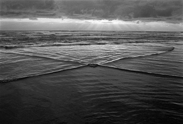
Figure 1. Interaction of line solitons. Oregon coast

We refer to [75] for the derivation of a new class of weakly transverse approximations of the water waves system in the Boussinesq regime which are purely local (without the anti-derivative in $x$), have a dispersion relation which fitting well with that of the original Euler system, and which provide optimal error estimates. No mass constraint has to be imposed there.

2.2. Localized solitary waves

Solitary waves are solutions of KP equations of the form

$$u(x,y^{\perp},t)=\psi_{c}(x-ct,y^{\perp}),$$

where $y^{\perp}$ ($=y$ or $(y,z))$ is the transverse variable and $c>0$ is the solitary wave velocity.

The solitary wave is said to be localized if $\psi_{c}$ tends to zero at infinity in all directions. For such solitary waves, the following energy space is natural

$$Y=Y(\mathbb{R}^{2})=\{u\in L^{2}(\mathbb{R}^{2}),\;u_{x}\in L^{2}(\mathbb{R}^{2}),\;\partial_{x}^{-1}u_{y}\in L^{2}(\mathbb{R}^{2})\},$$

(with an obvious modification in the three dimensional case),

and throughout this section we will deal only with finite energy solitary waves.

Due to its integrability properties, the KP I equation possesses a localized, finite energy, explicit solitary wave, the lump [84] :

(24) $$\phi_{c}(x-ct,y)=\frac{8c(1-\frac{c}{3}(x-ct)^{2}+\frac{c^{2}}{3}y^{2})}{(1+\frac{c}{3}(x-ct)^{2}+\frac{c^{2}}{3}y^{2})^{2}}.$$

Another interesting explicit solitary wave of the KP I equation which is localized in $x$ and periodic in $y$ has been found by Zaitsev [128]. It reads

(25) $$Z_{c}(x,y)=12\alpha^{2}\frac{1-\beta\cosh(\alpha x)\cos(\delta y)}{[\cosh(\alpha x)-\beta\cos(\delta y)]^{2}},$$

where

$$(\alpha,\beta)\in(0,\infty)\times(-1,+1),$$

and the propagation speed is given by

$$c=\alpha^{2}\frac{4-\beta^{2}}{1-\beta^{2}}.$$

Let us observe that the transform $\alpha\rightarrow i\alpha$, $\delta\rightarrow i\delta$, $c\rightarrow ic$ produces solutions of the KP I equation which are periodic in $x$ and localized in $y$.

We address first the question of non existence of solitary waves for the following classes of KP type equations

(26) $$u_{t}+u^{p}u_{x}+u_{xxx}+\epsilon\partial_{x}^{-1}u_{yy}=0,$$

where $\epsilon=\pm 1$, in the two-dimensional case, and

(27) $$u_{t}+u^{p}u_{x}+u_{xxx}+a\partial_{x}^{-1}u_{yy}+b\partial_{x}^{-1}u_{zz}=0,$$

where $a,b=\pm 1$, in the three-dimensional case.

By establishing suitable Pohojaev type identities, it has been proved in [19] that (under mild regularity conditions), no localized solitary waves exist when $c\leq 0$ in both dimensions and for $c>0$ when

$$\;\epsilon=-1,\;p\geq 4\quad\text{or}\quad\epsilon=1\;\text{and}\;p\;\text{arbitrary},$$

$$ab=-1\;(\text{resp.}\;a=b=1)\;\text{and}\;p\;\text{arbitrary},$$

or

$$a=b=-1,\;p\geq\frac{4}{3}.$$

In particular, the 2D KP II-type equations ($\epsilon=1,$ $p\geq 1$) do not possess any localized solitary waves. This was precised by de Bouard and Martel [18] who proved that the classical KP II equation does not possess $L^{2}$- compact solutions (those finite energy solutions are more general than solitary waves).

We refer to [19] for nonexistence results of localized solitary waves of KP type equations with a cubic-quintic dispersion in $x$.

We turn now to the existence of localized, finite energy solitary waves. We will consider as a basic example a class of generalized KP I equations in two dimensions of the form

(28) $$u_{t}+u^{p}u_{x}+u_{xxx}-\partial_{x}^{-1}u_{yy}=0,$$

where $p=\frac{m}{n},$  $n$ odd, $m$ and $n$ relatively prime.

Solitary waves are looked for in the energy space $Y(\mathbb{R}^{2})$ which can also be defined (see [19]) as the closure of the space of $x$ derivatives of smooth and compactly supported functions in $\mathbb{R}^{2}$ for the norm

$$\|\partial_{x}f\|_{Y(\mathbb{R}^{2})}\equiv\Big{(}\|\nabla f\|_{L^{2}(\mathbb{R}^{2})}^{2}+\|\partial_{x}^{2}f\|_{L^{2}(\mathbb{R}^{2})}^{2}\Big{)}^{\frac{1}{2}}.$$

The equation of a solitary wave $\psi$ of speed $c$ is given by

(29) $$c\partial_{x}\psi-\psi\partial_{x}\psi-\partial_{x}^{3}\psi+\partial_{x}^{-1}(\partial_{y}^{2}\psi)=0,$$

which implies

(30) $$c\partial_{xx}\psi-(\psi\partial_{x}\psi)_{x}-\partial_{x}^{4}\psi+\partial_{y}^{2}\psi=0,$$

When $\psi\in Y(\mathbb{R}^{2})$, the function $\partial_{x}^{-1}\partial_{y}^{2}\psi$ is well-defined (see [19]), so that (29) makes sense.

Given any $c>0$, a solitary wave $\psi_{c}$ of speed $c$ is deduced from a solitary wave $\psi_{1}$ of velocity $1$ by the scaling

(31) $$\psi_{c}(x,y)=c\psi_{1}(\sqrt{c}x,cy).$$

We now introduce the important notion of ground state solitary waves.

We set

$$E_{KP}(\psi)=\frac{1}{2}\int_{\mathbb{R}^{2}}(\partial_{x}\psi)^{2}+\frac{1}{2}\int_{\mathbb{R}^{2}}(\partial_{x}^{-1}\partial_{y}\psi)^{2}-\frac{1}{2(p+2)}\int_{\mathbb{R}^{2}}\psi^{p+2},$$

and we define the action

$$S(N)=E_{KP}(N)+\frac{c}{2}\int_{\mathbb{R}^{2}}N^{2}.$$

We term ground state, a solitary wave $N$ which minimizes the action $S$ among all finite energy non-constant solitary waves of speed $c$ (see [19] for more details).

It was proven in [19] that ground states exist if and only if $c>0$ and $1\leq p<4$. Moreover, when $1\leq p<\frac{4}{3},$ the ground states are minimizers of the Hamiltonian $E_{KP}$ with prescribed mass ($L^{2}$ norm).

Remark 3.

When $p=1$ (the classical KP I equation), it is unknown (but conjectured) whether the lump solution is a ground state.

In the three dimensional case, ground states exist when $a=b=-1$ and $1\leq p<\frac{4}{3}$ [19]. They are never minimizers of the corresponding energy with fixed $L^{2}$ norm (actually this minimization problem has no solutions in this case).

It turns out that qualitative properties of solitary waves can be established for a large class of KP type equations. Ground state solutions are shown in [20] to be cylindrically symmetric, that is radial with respect to the transverse variable up to a translation of the origin.

On the other hand, any finite energy solitary wave is infinitely smooth (at least when the exponent $p$ is an integer) and decay with an algebraic rate $r^{-2}$ in two dimension and $r^{-3+\epsilon}$ in dimension three [20]. Actually the decay rate is sharp in the sense that a solitary wave cannot decay faster that $r^{-d},$ $d=2,3.$

Moreover a precise asymptotic expansion of the solitary waves has been obtained by Gravejat ([33]).

The fact whether the ground states are or are not minimizers of the Hamiltonian is strongly linked to the orbital stability of the set $\mathcal{G}_{c}$ of ground states of velocity $c$. Note that the uniqueness, up to the obvious symmetries, of the ground state of velocity $c$ is a difficult open problem, even for the classical KP I equation.

Saying that $\mathcal{G}_{c}$ is orbitally stable in $Y$ means that for $\phi_{c}\in\mathcal{G}_{c},$ then for all $\epsilon>0,$ there exists $\delta>0$ such that if $u_{0}\in Y$ is such that $||u_{0}-\phi_{c}||_{Y}\leq\delta,$ then the solution $u(t)$ of the Cauchy problem initiating from $u_{0}$ satisfies

$$\sup_{t\geq 0}\inf_{\psi\in\mathcal{G}}||u(t)-\psi||_{Y}\leq\epsilon.$$

Actually it is proved in [21] that the ground state solitary waves are orbitally stable in dimension two if and only if $1\leq p<\frac{4}{3}$ while there are always unstable in dimension three.

We will see below the link between stability and blow-up in finite time of the solutions to the Cauchy problem.

Remark 4.

No rigorous stability (or instability) result seems to be known for the Zaitsev solitary wave solution of the KP I equation.

2.3. The linear group

As previously mentioned, the linear part associated to any KP type equations (18) generates a group $S(t)=\exp(t(\partial_{x}L+\partial^{-1}_{x}\partial^{2}_{yy}))$ which is unitary in all Sobolev spaces, in particular in $L^{2}$. For instance in the case of KP I/II equations, we have

$$S_{KPI/II}(t)=\exp(t(\partial_{xxx}\mp\partial_{x}^{-1}\partial^{2}_{yy}))$$

When the problem is set in $\mathbb{R}^{2}$, $S_{KPI/II}(t)$ has nice dispersive properties. In fact an analysis of the fundamental solution leads to the dispersive estimate [103]

(32) $$||S_{KPI/II}(t)\phi||_{L^{\infty}(\mathbb{R}^{2})}\leq\frac{C}{|t|}||\phi||_{L^{1}(\mathbb{R}^{2})},\quad\forall t\neq 0.$$

Such an estimate leads to $L^{p}_{t}L^{q}_{xy}$ Strichartz estimates [103] which are useful to solve the nonlinear Cauchy problem. Typically, one gets estimates of the type (here $S(t)$ stands for the KP I or the KP II group) :

(33) $$||S(t)\phi||_{L^{q}(\mathbb{R};L^{r}(\mathbb{R}^{2})}\leq C||\phi||_{L^{2}(\mathbb{R})},$$

for any $r\in[2,+\infty),$ and where $q=q(r)$ is defined by $\frac{1}{q}=\frac{1}{2}-\frac{1}{r}.$

Similar estimates hold for the “Duhamel integral”

$$\Lambda f(t)=\int_{0}^{t}S(t-s)f(s)ds.$$

Of course an estimate like (32) is false when the spatial domain is the torus $\mathbb{T}^{2}$ or the “mixed ” case $\mathbb{R}\times\mathbb{T}$ or $\mathbb{T}\times\mathbb{R}.$

On the other hand, dispersive estimates of the type (32) hold true when the $u_{xxx}$ dispersive term in the KP equation is replaced by $\partial_{x}P(\partial_{x})u,$ where $P$ is an even polynomial (see [9]), in particular for the “cubic-quintic” KP equations. In this case the corresponding Strichartz estimates involve a global smoothing effect [9].

Another interesting dispersive property of the KP group is the local smoothing property.

It has been known since the seminal paper of Kato [60] that the Airy group, that is $S(t)=e^{it\partial_{x}^{3}},$ satisfies the following local smoothing estimate

$$||\partial_{x}S(t)\phi)||_{L^{2}(0,T;L^{2}_{loc}(\mathbb{R})}\leq C||\phi||_{L^{2}(\mathbb{R}))}.$$

In other words there is (locally in space) a gain of one derivative.

A similar property was established in [103] for the KP II group. Actually, for any initial data $\phi\in L^{2}(\mathbb{R}^{2}),\;\partial_{x}^{-1}\phi\in L^{2}(\mathbb{R}^{2})$, the corresponding solution $u$ of the linear KP II equation satisfies the estimate, for any $T>0$ and $R>0$,

$$\int_{-T}^{T}\int_{-R}^{R}\int^{\infty}_{-\infty}[u_{x}^{2}(x,y,t)+|\partial_{x}^{-1}u_{y}(x,y,t)|^{2}]dxdydt\leq C(R,T)||\phi||^{2}_{L^{2}(\mathbb{R}^{2})},$$

which also displays a local gain of one derivative.

A stronger smoothing effect holds for the nonlinear KP II equation when the initial data decay fast to the right [79]. More precisely, if the initial data satisfies

$$\int_{\mathbb{R}^{2}}[\phi^{2}+\phi^{2}_{xxx}+(\partial_{x}^{-1}\phi_{yy})^{2}+x_{+}^{L}\phi^{2}+x_{+}^{L}\phi^{2}_{x}]dxdy<+\infty$$

for all positive integers $L$, then the corresponding solution $u$ (which exists globally, see the next Section) satisfies $u(.,t)\in C^{\infty}(\mathbb{R}^{2})$ for all positive $t$’s.

A result of this type (with different hypothesis on the initial data) was established in [78] for the nonlinear KP I equation.

2.4. The nonlinear Cauchy problem

All the KP type equations can be viewed as a linear skew-adjoint perturbation of the Burgers equation. Using this structure, it is not difficult (for instance by a compactness method) to prove that the Cauchy problem is locally well-posed for data in the Sobolev spaces $H^{s},$ $s>2$ in both dimensions (see [124], [103], [50] for results in this direction).

Unfortunately, this kind of result does not suffice to obtain the global well-posedness of the Cauchy problem. This would need to use the conservation laws of the equations. For general KP type equations, there are only two of them, the conservation of the $L^{2}$ norm and the conservation of the energy (Hamiltonian). For the general equation (8) where $f(u)=\frac{1}{p+1}u^{p+1},$ and without the transport term $u_{x}$ (which can be eliminated by a change of variable), the Hamiltonian reads

(34) $$E(u)=\frac{1}{2}\int\left[-u\,Lu+(\partial_{x}^{-1}u_{y})^{2}+\frac{u^{p+2}}{p+2}\right],$$

and for the classical KP I/II equations

(35) $$E(u)=\frac{1}{2}\int\left[u_{x}^{2}\pm(\partial_{x}^{-1}u_{y})^{2}-\frac{u^{3}}{3}\right],$$

where the $+$ sign corresponds to KP I and the $-$ sign to KP II.

Note that the “integrable” KP I and KP II equations possess more conservation laws, but not infinitely many as it is often claimed (see below).

In any case, it is clear that for KP II type equation, the Hamiltonian is useless to control any Sobolev norm, and to obtain the global well-posedness of the Cauchy problem one should consider $L^{2}$ solutions, a very difficult task. On the other hand, for KP I type equations, one may hope (for a not too strong nonlinearity) to have a global control in the energy space, that is

(36) $$E=\{u\in L^{2},\;uLu\in L^{2},\;\partial_{x}^{-1}u_{y}\in L^{2}\}.$$

For the usual KP I equation, $E=Y$, which was defined in the previous subsection.

The problem is thus reduced to proving the local well-posedness of the Cauchy problem in spaces of very low regularity, a difficult matter which has attracted a lot of efforts in the recent years.

Remark 5.

By a standard compactness method, one obtains easily the existence of global weak finite energy solutions (without uniqueness) to the KP I equation (see eg [119]).

At this point, there is a striking difference between the KP I and the KP II equation, linked to their different dispersion relations. The KP II equation can be solved by a Picard scheme implemented on the integral (Duhamel) formulation, implying that the flow map $u_{0}\mapsto u(.,t)$ is smooth in natural Sobolev spaces. In this sense the KP II equation can be viewed as a semi-linear equation.

On the other hand, it has been proved in [105] for the periodic case and in [92] for the Cauchy problem in $\mathbb{R}^{2}$ that the KP I equation cannot be solved by such a procedure, in any natural Sobolev class. This implies that the flow map cannot be smooth, and actually it cannot be even uniformly continuous on bounded sets of the natural energy space $Y$ (see [71]). This is a typical property of quasi-linear hyperbolic systems (eg the Burgers equation). It is thus natural to consider the KP I equation as a quasi-linear equation.

Those ill/well posedness by iteration properties have a huge importance when solving the Cauchy problem since the methods are quite different in both cases. We will first focus on the classical KP I and KP II equations.

For the KP II equation, a breakthrough was made by Bourgain [22] who proved that the Cauchy problem for the KP II equation is locally (thus globally in virtue of the conservation of the $L^{2}$ norm) for data in $L^{2}(\mathbb{R}^{2}),$ and even in $L^{2}(\mathbb{T}^{2}).$ This result was later improved ([117], [121], [122] [118], [53], [39], [40]) to allow the case of initial data in negative order Sobolev spaces.

Remark 6.

Bourgain’s proof uses in a crucial way the fact (both in the periodic and full space case) that the dispersion relation of the KP II equation induces the triviality of a certain resonant set. A similar property was used by Zakharov [130] to construct a Birkhoff formal form for the periodic KP II equation with small initial data. On the other hand, the fact that for the KP I equation the corresponding resonant set is non trivial is crucial in the construction of the counter-examples of [105], [92] and is apparently an obstruction to the Zakharov construction for the periodic KP I equation.

The KP II equation in three space dimensions has been studied in [121], [52]. The Cauchy problem is locally well-posed for initial data in anisotropic Sobolev spaces having $1^{+}$ derivative in $x$ and $0^{+}$ derivatives in $y,z$ in $L^{2}(\mathbb{R}^{3})$. It is an open problem whether or not those solutions are globally defined.

We refer to [103], [50], [39], [65], [66], [35], [43] for similar results on generalized KP II type equations. Note that for nonlinearities higher than quadratic, that is $f(u)=u^{p+1},\;p>1$ in (8), and $Lu=-u_{xx},$ one gets only the local well-posedness. Neither global existence nor blow-up in finite time are established.

On the other hand, global results are known to be true for higher order KP II equations, eg for the fifth order equation corresponding to $Lu=-u_{xxxx}$ [106].

Most of those results are based on iterative methods on the Duhamel formulation, using the Fourier restriction $X^{s,b}$ spaces of Bourgain, or variant of them, possibly with the injection of various linear dispersive estimates (see [103], [9]).

We also would like to mention the paper by Kenig and Martel [64] where the Miura transform is used to prove the global well-posedness of a modified KP II equation.

In view of [92] the situation is quite different for the KP I equation. Note however that the KP I equation with a fifth order dispersion in $x$ is globally well-posed in the corresponding energy space [107] (see also [37] for local well-posedness results without the “zero mass constraint” on the initial data).

For the classical KP I equation, the first global well-posedness result for arbitrary large initial data in a suitable Sobolev type space was obtained by Molinet, Saut and Tzvetkov [94]. The solution is uniformly bounded in time and space.

The proof is based on a rather sophisticated compactness method and uses the first invariants of the KP I equation to get global in time bounds. It is worth noticing that, while the recursion formula in [131] gives formally a infinite number of invariants, except for the first ones, those invariants do not make sense for functions belonging to $L^{2}(\mathbb{R}^{2})$ based Sobolev spaces.

For instance, the invariant which should control $||u_{xxx}(.,t)||_{L^{2}}$ contains the $L^{2}$ norm of $\partial_{x}^{-1}\partial_{y}(u^{2})$ which does not make sense for a non zero function $u$ in the Sobolev space $H^{3}(\mathbb{R}^{2})$. Actually (see [93], [94]), one checks easily that if $\partial_{x}^{-1}\partial_{y}(u^{2})\in L^{2}(\mathbb{R}^{2}),$ then $\int_{\mathbb{R}^{2}}\partial_{y}(u^{2})dx=\partial_{y}\int_{\mathbb{R}^{2}}u^{2}dx\equiv 0,\;\forall y\in\mathbb{R},$ which, with $u\in L^{2}(\mathbb{R}^{2}),$ implies that $u\equiv 0.$ Similar obstructions occur for the higher order “invariants”.

One is thus led to introduce a quasi-invariant (by skipping the non defined terms) which eventually will provide the desired bound. There are also serious technical difficulties to justify rigorously the conservation of the meaningful invariants along the flow and to control the remainder terms

The result of [94] was extended by Kenig [62] (who considered initial data in a larger space), and by Ionescu, Kenig and Tataru [49] who proved that the KP I equation is globally well-posed in the energy space $Y$.

Remark 7.

For both the KP I and KP II equations, the Inverse Scattering method provides only global well-posedness for small initial data. We refer to [127] for the KP II equation and to [132], [112] for the KP I equation.

Concerning the generalized KP I equations

(37) $$u_{t}+u_{xxx}-\partial_{x}^{-1}u_{yy}+u^{p}u_{x}=0,$$

an important remark is that the anisotropic Sobolev embedding (see [12])

$$\int_{\mathbb{R}^{2}}|u|^{p+2}dxdy\leq C||u||_{L^{2}}^{\frac{4-p}{2}}||u_{x}||_{L^{2}}^{p}||\partial_{x}^{-1}u_{y}||_{L^{2}}^{\frac{p}{2}},$$

which is valid for $0\leq p\leq 4,$ implies that the energy norm $||u||_{Y}$ is controlled in term of the $L^{2}$ norm and of the Hamiltonian

$$\int_{\mathbb{R}^{2}}\left(\frac{1}{2}u_{x}^{2}+\frac{1}{2}(\partial_{x}^{-1}u_{y})^{2}-\frac{|u|^{p+2}}{(p+1)(p+2)}\right)dxdy,$$

if and only if $p<\frac{4}{3}.$

This suggest global well-posedness when $p<\frac{4}{3}$ and blow-up when $p\geq\frac{4}{3}$, a fact which will be proved in the next Section.

2.5. Blow-up issues

We consider here a class of generalized KP equations

(38) $$u_{t}+u_{xxx}+\epsilon\partial_{x}^{-1}u_{yy}+u^{p}u_{x}=0,$$

where $\epsilon=1$ for the KP II equations and $-1$ for the KP I equations.

The KP I equations are focusing while the KP II are defocusing and to this aspect they share some properties with the focusing (resp. defocusing) nonlinear Schrödinger equation (NLS). In particular one could expect the blow-up in finite time of the solutions of generalized KP I equations with a sufficiently high nonlinearity.

For the focusing NLS, one can prove the blow-up in finite time of the $L^{2}$ norm of the spatial gradient by using a virial identity (see eg [111]). For the generalized KP I equation, one can use a “transverse” virial identity to prove the blow up in finite time of the $L^{2}$ norm of the transverse gradient (that is to say in $2D$ of $||u_{y}(.,t)||_{L^{2}(\mathbb{R}^{2})}).$ This identity has been formally derived in [120] and rigorously justified in [103] (one needs to prove a local well-posedness theory in a weighted $L^{2}$ space). It reads for solutions of the generalized KP equations in a suitable functional class:

(39) $$\frac{d^{2}}{dt^{2}}I(t)=4\epsilon[-pE(t)+\frac{p}{2}\int_{\mathbb{R}^{2}}u_{x}^{2}dxdy+\frac{(4-p)}{2}\epsilon\int_{\mathbb{R}^{2}}(\partial_{x}^{-1}u_{y})^{2}dxdy],$$

(40) $$E(t)=\int_{\mathbb{R}^{2}}[\frac{1}{2}(u_{x}^{2}-\epsilon(\partial_{x}^{-1}u_{y})^{2}-\frac{u^{p+2}}{(p+1)(p+2)}]dxdy,$$

and

$$I(t)=\int_{\mathbb{R}^{2}}y^{2}u^{2}dxdy.$$

A first direct consequence of (39) for KP I equations ($\epsilon=-1$) is that, when the initial data $u_{0}$ (is “regular” and) belongs to the space

$$\Sigma=\{\phi\in E,\;y\phi\in L^{2}(\mathbb{R}^{2}),\;\phi\neq 0,\;E(\phi)\leq 0\},$$

the corresponding solution of the Cauchy problem cannot remain smooth for all times if $p\geq 4.$ More precisely, there should exist $T^{*}>0$ such that

(41) $$\lim_{t\rightarrow T^{*}}||u_{y}(.,t)||_{L^{2}}=+\infty.$$

A similar result is obtained in the three-dimensional case ie when $\partial_{x}^{-1}u_{yy}$ in (38) is replaced by $\partial_{x}^{-1}\Delta^{\perp}u,$ where $\Delta^{\perp}$ is the transverse Laplacian in the $y$ and $z$ variables.

The critical value is then $p=2$ and (41) should be replaced by

(42) $$\lim_{t\rightarrow T^{*}}||\nabla^{\perp}u(.,t)||_{L^{2}}=+\infty.$$

Remark 8.

It is readily seen that the set $\Sigma$ is not empty. It contains in particular functions of the type $\pm\lambda\partial_{x}^{2}\exp(-x^{2}-y^{2})$ when $\lambda$ is a large positive number, the sign depending on the “parity” of $p$.

Those results are not fully satisfactory since we already observed that the natural energy norm is controlled by he $L^{2}$ norm and the Hamiltonian if and only if $0<p<\frac{4}{3}$ in the two-dimensional case. In the three dimensional case, the critical exponent is $p=\frac{4}{5}$ which suggests that the “standard” ($p=1)$ 3D- KP I equation is not supposed to have global solutions for arbitrary initial data.

This result was improved by Liu [81] who used invariant sets of the generalized KP I flow together with the virial argument above to prove the existence of initial data leading to blow-up in finite time of $||u_{y}(.,t)||_{L^{2}(\mathbb{R}^{2})}$ when $p\geq\frac{4}{3}$. He also proved a strong instability result of the solitary waves when $2<p<4.$

Similar results are established in [82] for the three-dimensional generalized KP I equation, in the range $1\leq p<\frac{4}{3}.$

Remark 9.

A detailed analysis of the blowing-up solution (profile, blow-up rate,..) is lacking.

Remark 10.

No rigorous finite time blow-up has been established for the periodic generalized KP I equation.

Remark 11.

No result seems to be known concerning the long time behavior (finite time blow-up versus global existence) of the solutions to the generalized KP II equations (38) when $\epsilon=1$ and $p\geq 2$).

Remark 12.

The finite time blow- up does not a priori invalidate the applicability of KP equations as asymptotic models. As all asymptotic models, they are supposed to describe the dynamics of a more general system, for a suitable scaling regime (here weakly nonlinear, long wave with a wavelength anisotropy) and on relevant (finite!) time scales. For instance, in the water wave context, the KP equations cease to be relevant models for times larger than $O(\frac{1}{\epsilon^{2}})$.

2.6. The Cauchy problem in the background of a non localized solution.

As was previously noticed, it is quite natural in view of transverse stability issues to consider the Cauchy problem for KP equations on the background of a solitary wave of the underlying KdV equation.

The Inverse Scattering method has been used formally in [4] and rigorously in [5] to study the Cauchy problem for the KP II equation with non decaying data along a line, that is $u(0,x,y)=u_{\infty}(x-vy)+\phi(x,y)$ with $\phi(x,y)\to 0$ as $x^{2}+y^{2}\to\infty$ and $u_{\infty}(x)\to 0$ as $|x|\to\infty$. Typically, $u_{\infty}$ is the profile of a traveling wave solution $U({\bf k}.{\bf x}-\omega t)$ with its peak localized on the moving line ${\bf k}.{\bf x}=\omega t.$ It is a particular case of the $N$- soliton of the KP II equation discovered by Satsuma [102] (see the derivation and the explicit form when $N=1,2$ in the Appendix of [97]). As for all results obtained for KP equations by using the Inverse Scattering method, the initial perturbation of the non-decaying solution is supposed to be small enough in a weighted $L^{1}$ space (see [5] Theorem 13). A similar result has been established by Fokas and Pogrebkov [29] for the KP I equation.

On the other hand, PDE techniques allow to consider arbitrary large perturbations of a class of non-decaying solutions of the KP I/II equations.

We will therefore study the initial value problem for the KP I and KP II equations

(43) $$(u_{t}+u_{xxx}+uu_{x})_{x}\pm u_{yy}=0,$$

where $u=u(t,x,y)$, $(x,y)\in\mathbb{R}^{2}$, $t\in\mathbb{R}$, with initial data

(44) $$u(0,x,y)=\phi(x,y)+\psi_{c}(x,y),$$

where $\psi_{c}$ is the profile of a non-localized (i.e., not decaying in all spatial directions) traveling wave of the KP I/II equations moving with speed $c\neq 0$.

We recall that, contrary to the KP I equation, the KP II equation does not possess any localized in both directions traveling wave solution.

The background solution $\psi_{c}$ could be for instance the line soliton (1-soliton) of the Korteweg- de Vries (KdV) equation (14), or the N-soliton solution of the KdV equation, $N\geq 2,$ or in the case of the KP I equation, the Zaitsev soliton.

The KdV N-soliton is of course considered as a two dimensional (constant in $y$) object.

This problem can be attacked in two different ways. Either one considers a localized (in $x$ and $y$) perturbation, or the perturbation is localized in $x$ and periodic in $y$.

Both frameworks have been applied to the KP I and KP II equations, and they lead to global well-posedness of the Cauchy problem for arbitrary large initial perturbations. More precisely, for the KP I equation, the Cauchy problem with initial data which are localized perturbations of the KdV N-soliton or of the Zaitsev soliton is globallly well-posed [95]. The corresponding result for the KP II equation is proved in [96].

The global well-posedness of the KP II equation with arbitrary initial data in $L^{2}(\mathbb{R}\times\mathbb{T})$ is proved in [96]. The corresponding result for the KP I equation with initial data in a suitable Sobolev space is established in [48].

2.7. Transverse stability issues

The KP I and KP II equations behave quite differently with respect to the transverse stability of the KdV $1$-soliton.

Zakharov [129] has proven, by exhibiting an explicit perturbation using the integrability, that the KdV $1$-soliton is nonlinearly unstable for the KP I flow. Rousset and Tzvetkov [101] have given an alternative proof of this result, which does not use the integrability, and which can thus be implemented on other problems (eg for nonlinear Schrödinger equations).

The nature of this instability is not known (rigorously) and it will be investigated in our numerical simulations.

On the other hand, Mizomachi and Tzvetkov [89] have recently proved the $L^{2}(\mathbb{R}\times\mathbb{T})$ orbital stability of the KdV $1$-soliton for the KP II flow. The perturbation is thus localized in $x$ and periodic in $y$. The proof involves in particular the Miura transform used in [64] to established the global well-posedness for a modified KP II equation.

Such a result is not known (but expected) for a perturbation which is localized in $x$ and $y$.

2.8. Comparison between the KP and KP/BBM type equations

As previously noticed, the KP/BBM equations (10) are relevant counterparts to KP type equations, for instance to the KP II equation

The Cauchy problems for those regularized KP equations has been studied in [108], for initial data in the natural energy space. We refer also to [16] for more regular initial data and for a stability analysis of the solitary waves in the focusing case.

The comparison of the dynamics of the KdV and BBM equation has been investigated both theoretically and numerically in [17]. A similar study was made in [86] between the KP and KP/BBM equations. Recall that KdV and BBM (resp. KP and KP/BBM) equations are supposed to describe the same dynamics, on relevant time scales.

2.9. Long time dynamics

KP type equations can be classified into two categories, the defocusing ones (KP II type), and the focusing ones (KP I type). For the former, the long time dynamics is expected to be governed by dispersion and scattering. In particular, at least for small initial data the $\sup$ norm should decay with the linear rate, that is $1/t$ (see [103]).

On the other hand, the dynamics of the latter case is expected to be governed by the solitary waves and blow-up in finite time is expected in the supercritical case. To this extent the situation is reminiscent of that of the nonlinear Schrödinger equations [111].

Relatively few mathematical results are know concerning those issues, and one goal of the present paper is to present numerical simulations in support of (or in motivation of) various conjectures on the long time dynamics.

For the generalized KP equation

$$u_{t}+u_{xxx}\pm\partial_{x}^{-1}u_{yy}+u^{p}u_{x}=0,$$

it was proven in [43] that if $p\geq 2$ and if the initial data is sufficiently small, then

$$||u(t)||_{\infty}\leq C(1+|t|)^{-1}(\log(2+|t|)^{\kappa},\quad||u_{x}(t)||_{\infty}\leq C(1+|t|)^{-1},$$

for all $t\in\mathbb{R}$, where $\kappa=1$, if $p=2$ and $\kappa=0$ if $p\geq 3.$

Moreover, a large time asymptotic for $u_{x}$ can be obtained.

Remark 13.

No such result seems to be known for the KP II equation, $p=1$ (see however Theorem 9.3 in [130] for a scattering result with small initial data by Inverse Scattering methods). We also mention [40] where a scattering result for small data in the scale invariant non isotropic homogeneous Sobolev space $\dot{H}^{-1/2,0}(\mathbb{R}^{2})$ is obtained.

The large time behavior of solutions to the KP II equation with arbitrary large data is unknown. An interesting open problem is that of possible uniform in time bounds on the higher Sobolev norms. It has been proven in [54] that the eventual growth in time of Sobolev norms is at most polynomial (see also [123] for long time bounds for the periodic KP II equation).

The long time dynamics of KP I type equations for arbitrarily large data is also an important open problem. For the standard KP I equation, it is expected that the ground state solutions (whether or not the lump is one of them) should play a role in this dynamics as the KdV solitary waves for the corresponding equation.

2.10. Initial data in the Schwartz class

One can prove that the Schwartz space $\mathcal{S}(\mathbb{R}^{d})$ of $C^{\infty}$ functions with rapid decay is not preserved by the (linear and nonlinear) flows of KP type equations, in fact the rapid decay is not preserved as it is easily seen on the solution of the linear KP I or KP II equations which reads in Fourier variables

$$\hat{u}(\xi_{1},\xi_{2},t)=\hat{u_{0}}(\xi_{1},\xi_{2})\exp(it(\xi_{1}^{3}\pm\frac{\xi_{2}^{2}}{\xi_{1}}))$$

Taking for instance $u_{0}$ equal to a gaussian function, one sees that $u(.,t)$ is not even in $L^{1}(\mathbb{R}^{2})$ for $t\neq 0$ since this would imply by Riemann-Lebesgue theorem that $\hat{u}(.,t)$ is a continuous function of $\xi$ which obviously is not the case. This proves in particular that the solution at time $t$ cannot decay faster than $\frac{1}{r^{2}}$ at infinity, where $r=\sqrt{x^{2}+y^{2}}.$ The same conclusion can be drawn in the nonlinear case. In fact the solution of the nonlinear equation with the same gaussian initial data has the Duhamel representation in Fourier variables

$$\hat{u}(\xi_{1},\xi_{2},,t)=\hat{u_{0}}(\xi_{1},\xi_{2})\exp(it(\xi_{1}^{3}\pm\frac{\xi_{2}^{2}}{\xi_{1}}))+\frac{i}{2}\int_{0}^{t}\xi_{1}\exp(i(t-s)(\xi_{1}^{3}\pm\frac{\xi_{2}^{2}}{\xi_{1}}))\widehat{u^{2}}(\xi_{1},\xi_{2},s)ds$$

and one checks that the integral part defines, for any fixed $t>0$, a continuous function of $\xi$ while the free part is not continuous as shown previously.

A stronger decay of solutions is obtained when extra (rather unphysical) conditions are imposed on the initial data $u_{0}$, namely the vanishing of $\widehat{u_{0}}(\xi_{1},\xi_{2})$ at higher and higher order as $\xi_{1}\to 0.$

The proofs above extend to any KP type equation like (8), the crux of the matter being the singularity at $\xi_{1}=0$ of the kernel $\frac{\xi_{2}^{2}}{\xi_{1}}.$

The fact that the solutions of KP type equations do not decay fast at infinity yields difficulties discussed in Section 3.1 for the realistic numerical simulations of the solutions in the whole space.

2.11. Varia

We mention briefly here a few other mathematical questions concerning KP type equations.

Many papers have been recently devoted to the study of initial boundary-value problems for various dispersive equations such as the KdV equation, motivated in particular by applications to control theory.

A IBV problem for the KP II equation on a strip or a half space has been studied in [87]. We do not know of any similar result for the KP I equation.

Many works have been recently devoted to the control or stabilization of linear or nonlinear dispersive equation.

We are not aware of any work on the control of (linear or nonlinear) KP type equations. A unique continuation property (which could be useful in control theory) for the KP II equation is established in [98]. A corresponding result for the KP I equation does not seem to be known.

As was previously alluded to in the context of water waves, one sometimes need for physical reasons to add a viscous term to the KP equations leading to interesting mathematical problems. For a viscous term of the Burgers type, that is $-u_{xx}$, Molinet and Ribaud [91] have established the global well-posedness of the Cauchy problem for data in $L^{2}(\mathbb{R}^{2})$ for the KP-II-Burgers equation and in the energy space $Y$ for the KP-I-Burgers equation. This result has been extended by Kojok [72] in the case of the KP-II-Burgers equation for initial data in the anisotropic Sobolev space $H^{s,0}(\mathbb{R}^{2})$, for any $s>-\frac{1}{2}.$

A sharp decay asymptotic analysis of the solutions of KP-Burgers equations as $t\to+\infty$ is carried out in [90].

3. Numerical study of generalized KP equations

In this section we will numerically study the stability of exact solutions to the KP equations for various perturbations, and the blow-up phenomenon in generalized KP equations.

3.1. General setting

We will now study numerically the solution to initial value problems for the generalized KP equations (38). We will only consider functions $u$ that are periodic in $x$ and $y$ with period $L_{x}2\pi$ and $L_{y}2\pi$ respectively or in the Schwartzian space of rapidly decreasing functions, which are essentially periodic for numerical purposes if restricted to an interval of length $L$ on which the functions decrease below values that can be numerically distinguished from zero ($10^{-16}$ in double precision). As noted in subsection 2.1, all solutions of (38) satisfy in this case for $t>0$ the constraint $\int_{-\pi L_{x}}^{\pi L_{x}}u_{yy}dx=0$. To obtain solutions which are smooth at time $t=0$ (for convenience we only consider times $t\geq 0$), the initial data also have to satisfy this constraint. It is possible to numerically solve initial value problems which do not satisfy the constraint, see for instance [68], but the non-regularity in time is numerically difficult to resolve. Therefore we will only consider initial data that satisfy this condition, typically by imposing that $u_{0}(x,y)$ is the $x$-derivative of a periodic or Schwartzian function. This even holds for perturbations of exact solutions we will consider in the following.

The imposed periodicity on the solutions allows the use of Fourier spectral methods. Equation (38) is equivalent to

(45) $$\partial_{t}\,\widehat{u}+\frac{i\xi_{1}}{p+1}\widehat{u^{p+1}}-i\xi_{1}^{3}\,\widehat{u}+\lambda\frac{i\xi_{2}^{2}}{\xi_{1}+i0}\,\widehat{u}=0.$$

The singular multiplier $-i/\xi_{1}$ is regularized in standard way as $-i/(\xi_{1}+i0)$. Numerically this is achieved by computing $-i/(\xi_{1}+i\epsilon)$ where $\epsilon$ is some small number of the order of the rounding error. Since we only consider functions $u$ satisfying the constraint $\xi_{2}^{2}\widehat{u}(t,\xi_{1}=0,\xi_{2})=0$, this does not lead to any numerical problems.

For a numerical solution equations (45) are approximated by a truncated Fourier series, i.e., a discrete Fourier transform for which fast algorithms exist. With this approximation one obtains a system of ordinary differential equations for which an initial value problem has to be solved. This system is stiff due to the high order spatial derivatives, especially since we want to resolve strong gradients. Standard explicit schemes would require prohibitively small time steps for stability reasons in this case, whereas unconditionally stable implicit schemes are typically not efficient, especially if one aims at high precision. In [67] we compared several fourth order schemes for the KdV equation, and in [70] a similar analysis was performed for KP. It was found that exponential time differencing schemes are most efficient in this case, see for instance the reviews [88],[44]. There are several such schemes known in the literature which show similar performance. We use here the fourth order scheme proposed by Cox and Matthews [25].

As noted in subsection 2.10, solutions to generalized KP equations for Schwartzian initial $u_{0}$ in general will not stay in the Schwartz class, unless $u_{0}$ satisfies in addition an infinite number of constraints. For generic initial data, the solutions $u(t)$ will develop ‘tails’ decaying only algebraically in certain spatial directions. This implies for the used periodic setting that Gibbs phenomena will appear on the borders of the computational domain for larger times. These jump discontinuities affect the numerical accuracy. Thus a much higher resolution than for KdV (where solutions to Schwartzian initial data stay in the Schwartz space) would be needed to obtain high numerical precision. In the below computations this effect is addressed by choosing a larger computational domain than would be necessary for similar KdV computations. The algebraic tails will lead due to the periodicity condition to ‘echoes’ which are, however, in most cases of comparatively small amplitude.

The numerical accuracy of the computations is controlled by propagating exact solutions and by computing conserved quantities of KP which are numerically functions of time due to unavoidable numerical errors, see [70]. As discussed before generalized KP equations conserve the $L^{2}$-norm (or mass) and the energy (40). Since the latter quantity contains the term $\partial_{x}^{-1}\partial_{y}u(t,x,y)$ which implies in Fourier space a division by $\xi_{1}$, an operation that affects accuracy in the determination of the quantity, we will trace mass conservation. In [70] it was shown that relative mass conservation $\Delta:=|1-M(t)/M(0)|$ ($M$ being the numerically $L^{2}$-norm) overestimates typically the accuracy of the numerical solution in an $L^{\infty}$ sense by 2 orders of magnitude. Thus we always aim at a $\Delta$ smaller than $10^{-4}$ to ensure accuracy of plotting precision. Obviously the quantity $\Delta$ only makes sense if the spatial numerical resolution is of the same order, i.e., if the Fourier coefficients $\widehat{u}(t,\xi_{1},\xi_{2})$ decrease for large $\xi_{1},\xi_{2}$ to the same order of magnitude. The precision of the computations will therefore always be controlled by mass conservation and Fourier coefficients. In addition we check whether the found numerical results remain the same within the considered accuracy if computed with higher or lower resolution.

Exact solutions to the KdV equation are automatically solutions to both KP equations without explicit $y$-dependence. Thus KdV solitons are line solitons of KP, i.e., solutions that are exponentially localized in one spatial direction and infinitely extended in the other. As mentioned above the KdV soliton (14) is unstable for KP I and lineary stable for KP II. To test the code we first propagate initial data from the KdV soliton $u_{0}=u_{sol}(x-x_{0})$ for $c=4$ and $x_{0}=-2L_{x}$ ($L_{x}=8$ and $L_{y}=8$, $x\in[-\pi,\pi]L_{x}$, $y\in[-\pi,\pi]L_{y}$) with $N_{x}=2^{8}$ and $N_{y}=2^{10}$ Fourier modes with $N_{t}=3200$ time steps from $t=0$ until $t=6$. For both KP I and KP II we find at $t=6$ that the relative mass conservation $\Delta=3.89*10^{-8}$ and that the $L^{\infty}$-norm of the difference between numerical and exact solution is equal to $9.96*10^{-7}$. This shows that the code is well able to propagate the exact solution even for the unstable case. It also illustrates that the quantity $\Delta$ can be used as expected as an indicator for the numerical accuracy. In the following subsections we will test how periodic perturbations of order unity of the KdV soliton are propagated by the KP equations.

3.2. Perturbations of the KdV soliton for KP II

The similarity between KP I and KP II for the exact KdV soliton initial data disappears if we perturb these data for instance by

(46) $$u_{p}=6(x-x_{1})\exp(-(x-x_{1})^{2})\left(\exp(-(y+L_{y}\pi/2)^{2})+\exp(-(y-L_{y}\pi/2)^{2})\right).$$

The perturbations are Schwartzian in both variables and satisfy the constraint (2.1). They are of the same order of magnitude as the KdV soliton, i.e., of order $0(1)$, and thus test the nonlinear stability of the KdV soliton.

Notice that the computations are carried out on a doubly periodic setting, i.e., $\mathbb{T}^{2}$ and not on $\mathbb{R}^{2}$. Thus the perturbations cannot be radiated to infinity, but will stay in the computational domain. Since they are of a similar size as the initial soliton, they will lead to a perturbed soliton though the KdV soliton is known to be stable for KP II. One possibility is that the initial perturbation is essentially homogeneously distributed over the whole computational domain. Another possibility would be that they form eventually a KdV soliton which is, however, not observed in the below examples.

For KP II we use the same parameters for the computation as for the tests for the KdV soliton, but now for initial data $u_{0}(x,y)=12\mbox{sech}^{2}(x+2L_{x})-u_{p}$ ($x_{1}=x_{0}/2$), i.e., a superposition of the KdV soliton and the not aligned perturbation. At time $t=6$ we obtain for the numerical conservation of the mass $\Delta=4.29*10^{-8}$, almost the same precision as for the propagation of the soliton. The result can be seen in Fig. 2. The perturbation is dispersed in the form of tails to infinity which reenter the computational domain because of the imposed periodicity. The soliton appears to be unaffected by the perturbation which eventually seems to be smeared out in the background of the soliton.

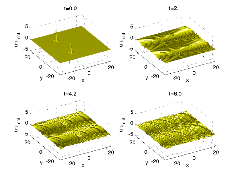
Figure 2. Difference of the solution to the KP II equation for initial data given by the KdV soliton plus perturbation, $u(0,x,y)=u_{sol}(x+2L_{x},0)$ and perturbation $u_{p}=6(x-x_{1})\exp(-(x-x_{1})^{2})\left(\exp(-(y+L_{y}\pi/2)^{2})+\exp(-(y-L_{y}\pi/2)^{2})\right)$, $x_{1}=-L_{x}$ and the KdV soliton for various values of $t$.

The situation changes slightly if the perturbation and the initial soliton are centered around the same $x$-value initially, i.e., the same situation as above with $x_{1}=x_{0}=-2L_{x}$. In Fig. 3 we show the difference between the numerical solution and the KdV soliton $u_{sol}$ for several times for this case.

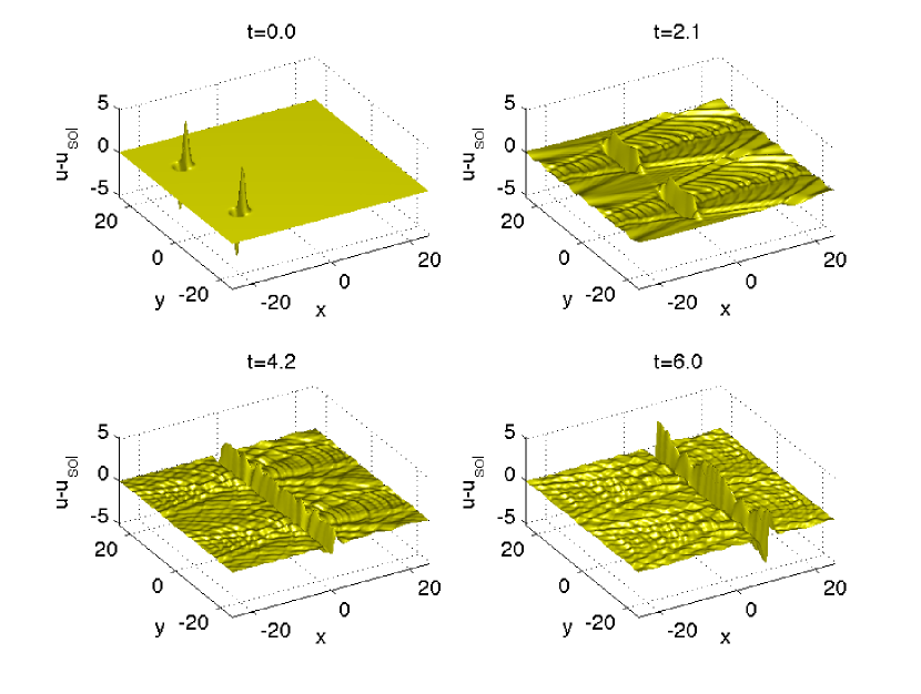
Figure 3. Difference of the solution to the KP II equation for initial data given by the KdV soliton $u_{sol}(x+2L_{x},0)$ plus perturbation $u_{p}=6(x-x_{1})\exp(-(x-x_{1})^{2})\left(\exp(-(y+L_{y}\pi/2)^{2})+\exp(-(y-L_{y}\pi/2)^{2})\right)$, $x_{1}=-2L_{x}$, and the KdV soliton for various values of $t$.

It can be seen that the initially localized perturbations spread in $y$-direction, i.e., orthogonally to the direction of propagation and take finally themselves the shape of a line soliton. The perturbations appear to modulate the soliton here. It is difficult numerically to determine the long time behavior. Extending the computation till time $t=16$, one finds a similar behavior as for $t=6$ as can be seen in Fig. 4.

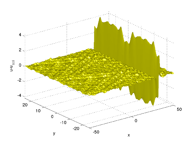
Figure 4. Difference of the solution to the KP II equation for the situation of Fig. 3 and the initial KdV soliton for $t=16$.

Thus it appears that the perturbations of the KdV soliton travel here partly with the soliton and lead to oscillations around it. Since the speed of the soliton is not affected, it is still the original, not a soliton with slightly increased $c$ which would change both height and speed of the traveling wave. But these perturbations traveling with the soliton seem to be present for very long times.

A similar behavior is observed if the soliton shape itself is deformed, for instance in the form of the initial data $u_{0}(x)=12\mbox{sech}^{2}(x+0.4\cos(2y/L_{y}))$. In Fig. 5 the difference of the solution for KP II for this initial data and the line soliton can be seen. The computation is carried out with $N_{x}=2^{10}$, $N_{y}=2^{7}$, $L_{x}=16$, $L_{y}=8$ and $N_{t}=6400$ with a final $\Delta\sim 10^{-7}$. It can be seen that the solution approaches the KdV soliton with perturbations oscillating around it.

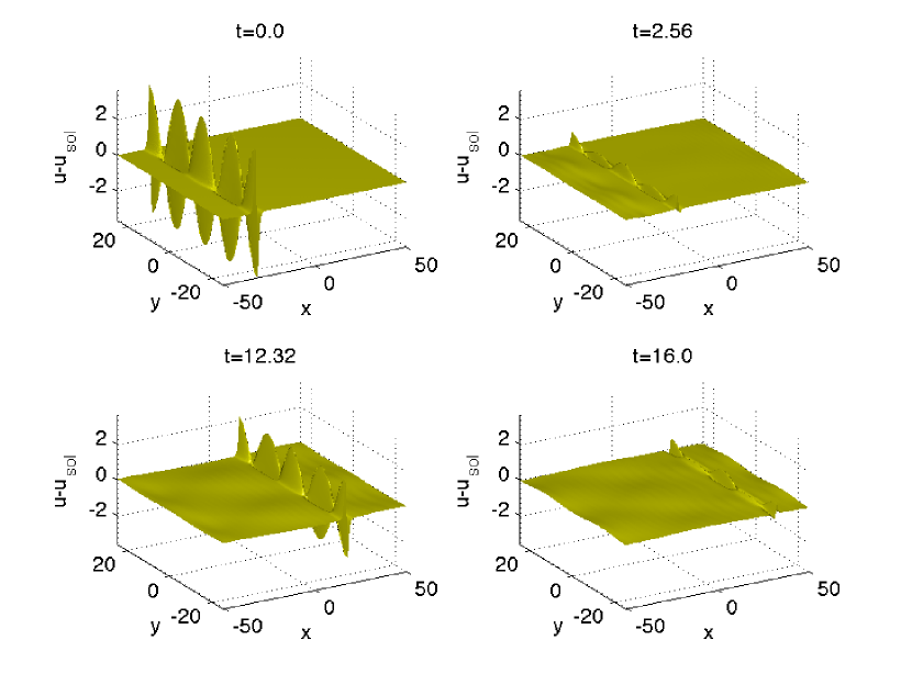
Figure 5. Difference of the solution to the KP II equation for the initial data $u_{0}(x)=12\mbox{sech}^{2}(x+0.4\cos(2y/L_{y}))$ and the KdV soliton for several values of $t$.

This is even more visible in Fig. 6 where the $L^{\infty}$-norm of the solution is given. It can be seen that the latter oscillates around the value for the KdV soliton. Numerically it is difficult to decide whether these oscillations will finally disappear.

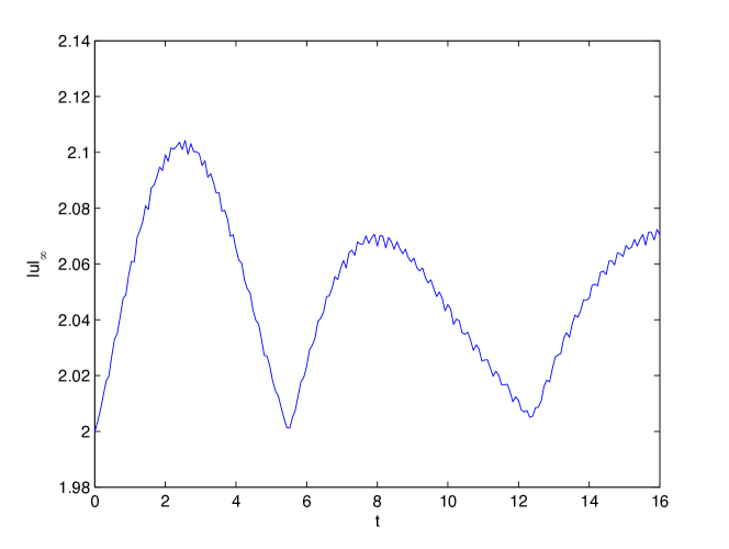
Figure 6. $L^{\infty}$-norm of the solution to the KP II equation for the situation of Fig. 5 in dependence of $t$.

3.3. Perturbations of the KdV soliton for KP I

Perturbations of the KdV soliton are propagated in a completely different way by the KP I equation. It is known that the line soliton is unstable for this equation. One of the reasons for this is the existence of lump solitons (24). Note that the lump soliton only decays algebraically in both spatial directions, as $|x|,|y|\to\infty$. Because of this and the ensuing Gibbs phenomena in the periodic setting used here for the numerical simulations, the appearance of lumps will always lead to a considerable drop off in accuracy. In contrast to the line solitons it is localized in both spatial directions. Explicit solutions for multi-lumps are known, see [84]. It was shown by Ablowitz and Fokas [2] that solutions to the KP I equation with small norm will asymptotically decay into lumps and radiation.

Exactly this behavior can be seen in Fig. 7 for the perturbed initial data of a line soliton with the perturbation (46) and $x_{1}=x_{0}=-2L_{x}$, i.e., the same setting as studied in Fig. 3 for KP II. Here the initial perturbations develop into 2 lumps which are traveling with higher speed than the line soliton. The formation of these lumps essentially destroys the line soliton which leads to the formation of further lumps. It appears plausible that for sufficiently long times one would only be able to observe lumps and small perturbations which will be radiated to infinity if studied on $\mathbb{R}^{2}$.

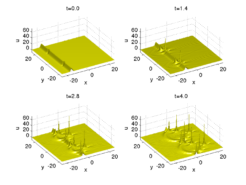
Figure 7. Solution to the KP I equation for initial data given by the KdV soliton $u_{sol}(x+2L_{x},0)$ plus perturbation $u_{p}=6(x-x_{1})\exp(-(x-x_{1})^{2})\left(\exp(-(y+L_{y}\pi/2)^{2})+\exp(-(y-L_{y}\pi/2)^{2})\right)$, $x_{1}=-2L_{x}$, for various values of $t$.

Notice that the algebraic fall off towards infinity causes the above mentioned numerical problems. This is reflected by the fact that the Fourier coefficients decrease much slower than in the case of KP II such that $N_{x}=2^{9}$ and $N_{y}=2^{10}$ Fourier modes are needed to ensure that the Fourier coefficients go down by at least 5 orders of magnitude in $\xi_{1}$ and $\xi_{2}$. For the relative mass conservation one obtains $\Delta=4.3*10^{-5}$ with $N_{t}=6400$.

We can give some numerical evidence for the validity of the interpretation of the peaks in Fig. 7 as lumps in an asymptotic sense. We can identify numerically a certain peak, i.e., obtain the value and the location of its maximum. With these parameters one can study the difference between the KP solution and a lump with these parameters to see how well the lump fits the peak. This is illustrated for the two peaks, which formed first and which have therefore traveled the largest distance in Fig. 8.

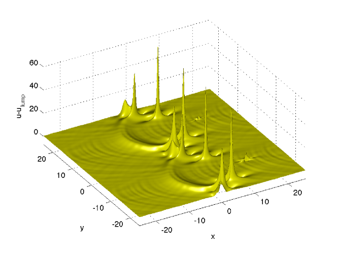
Figure 8. Difference of the solution to the KP I equation in Fig. 7 for $t=4$ and two lump solutions fitted at the peaks farthest to the right. Only very small peaks remain of these ‘lumps’ indicating that they develop asymptotically into true lumps.

Obviously one cannot expect a true lump in this case since there are still some remains of the line soliton to be seen. A multi-lump solution might be a better fit, but here we mainly want to illustrate the concept which obviously cannot fully apply at the studied small times. Nonetheless Fig. 8 illustrates convincingly that the observed peaks will asymptotically develop into lumps.

The precise pattern of lumps forming obviously depends on the perturbation. In Fig. 9 one can see the KP I solution for the same situation as in Fig. 7 except for the different sign of the perturbation $u_{p}$ (46). In this case two pairs of lump form first to be followed at later times by a collection of lumps.

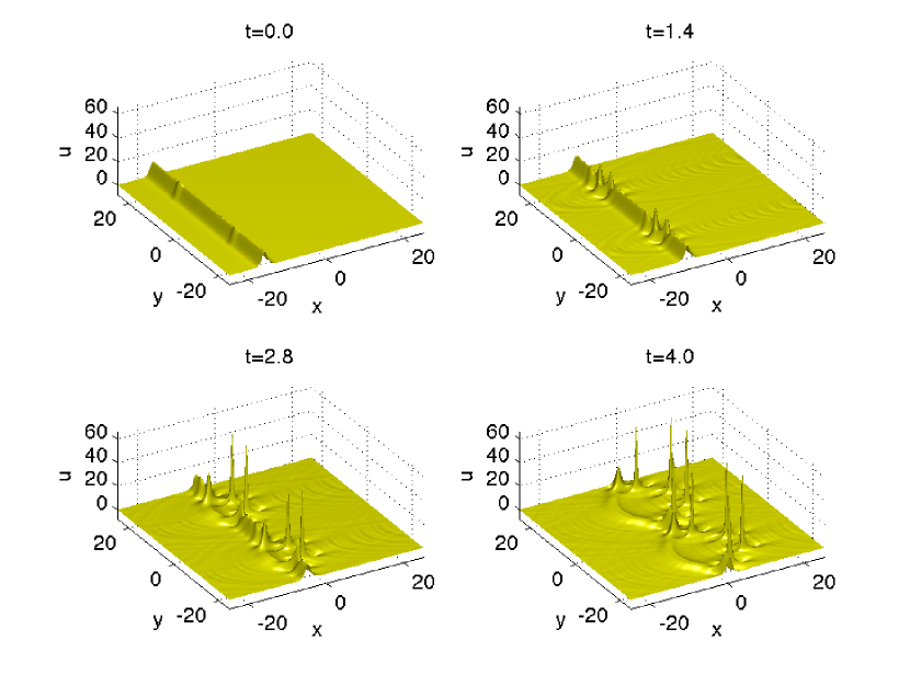
Figure 9. Solution to the KP I equation for initial data given by the KdV soliton $u_{sol}(x+2L_{x},0)$ plus perturbation $u_{p}=-6(x-x_{1})\exp(-(x-x_{1})^{2})\left(\exp(-(y+L_{y}\pi/2)^{2})+\exp(-(y-L_{y}\pi/2)^{2})\right)$, $x_{1}=-2L_{x}$, for various values of $t$.

Perturbing the line soliton in the form $u_{0}(x)=12\mbox{sech}^{2}(x+0.4\cos(2y/L_{y}))$, one finds the solution shown in Fig. 10. Two lumps form at the deformed line soliton farthest to the right. Further lumps then form at later times where the first detached from the deformed soliton. It appears that the perturbation develops in this case into a chain of lumps. The computation is carried out with $N_{x}=N_{y}=2^{11}$ modes and $10^{4}$ time steps for $L_{x}=16$ and $L_{y}=8$. Due to the propagation of lumps of large magnitude for an extended time, the relative mass conservation is comparatively low in this case, $\Delta\sim 3*10^{-3}$.

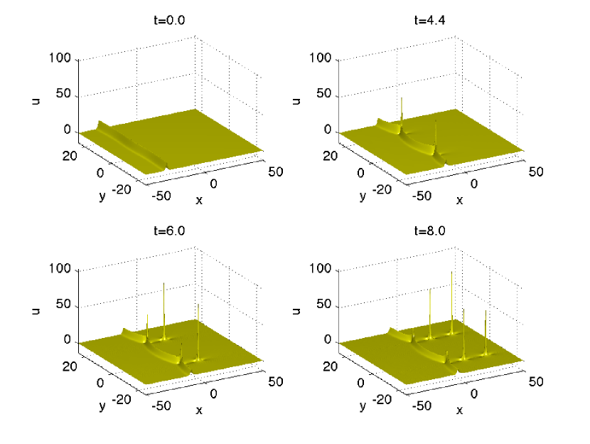
Figure 10. Solution to the KP I equation for initial data $u_{0}(x)=12\mbox{sech}^{2}(x+0.4\cos(2y/L_{y}))$ for various values of $t$.

The above numerical experiments indicate that the line soliton is unstable against general perturbations. Whereas this might be true on long time scales, this is not necessarily the case on intermediate time scales. To illustrate this ‘meta-stability’ we consider in Fig. 11 a perturbation of the line soliton as before $u_{0}(x,y)=12\mbox{sech}^{2}(x+2L_{x})+u_{p}$, but this time with $x_{1}=x_{0}/2$, i.e., perturbation and soliton are well separated.

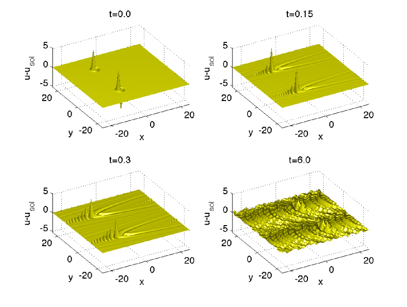
Figure 11. Difference of the solution to the KP I equation for initial data given by the KdV soliton $u_{sol}(x+2L_{x},0)$ plus perturbation $u_{p}=6(x-x_{1})\exp(-(x-x_{1})^{2})\left(\exp(-(y+L_{y}\pi/2)^{2})+\exp(-(y-L_{y}\pi/2)^{2})\right)$, $x_{1}=-L_{x}$ and the KdV soliton for various values of $t$.

The figure shows the difference between KP I solution and line soliton. It can be seen that the soliton is essentially stable on the shown time scales. The perturbation leads to algebraic tails towards positive $x$-values and to dispersive oscillations as studied in [68]. Due to the imposed periodicity both of these cannot escape the computational domain and appear on the respective other side. The important point is, however, that though the oscillations of comparatively large amplitude hit the line soliton quickly after the initial time, its shape is more or less unaffected till $t=6$.

The picture changes, however, if the code runs for a longer time as can be seen in Fig. 12. The soliton develops for times greater than 6 lumps after having stayed close to its original shape before despite strong perturbations. The solution for times greater than 6 remains the same within the given precision if the resolution is changed. For instance if we compare the result with $N_{t}=6400$ and $N_{t}=12800$, the maximal difference between the numerical solutions if of the order $10^{-4}$. The quantity $\Delta$ in the latter case is of the order of $10^{-8}$, whereas the Fourier coefficients decrease to $10^{-8}$. Doubling the resolution in $x$ leads to a difference of the order of $10^{-9}$ between the solutions. Thus one can conclude that the above solution is in fact correct within numerical precision.

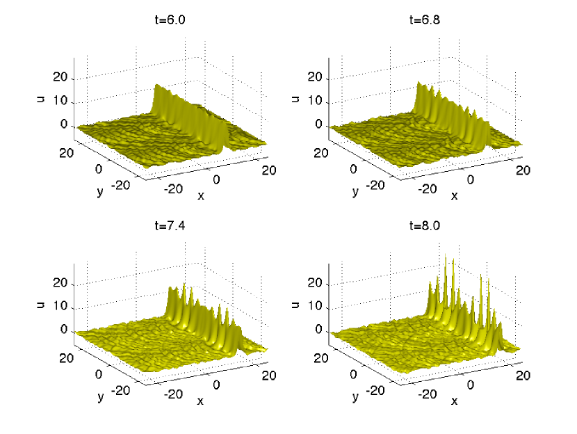
Figure 12. Solution to the KP I equation for initial data given by the KdV soliton $u_{sol}(x+2L_{x},0)$ plus perturbation $u_{p}=6(x-x_{1})\exp(-(x-x_{1})^{2})\left(\exp(-(y+L_{y}\pi/2)^{2})+\exp(-(y-L_{y}\pi/2)^{2})\right)$, $x_{1}=-L_{x}$ and the KdV soliton for various values of $t$.

Of course the periodic setting has an important effect here. Changing $L_{y}$ from 8 to 10 whilst keeping all other parameters unchanged does not affect the solution within the given precision. However the picture changes if we pass from $L_{x}=8$ to $L_{x}=10$ as can be seen in Fig. 13. At time $t=8$ the soliton is still mainly unperturbed, and only then the lump formation starts. This implies that the instability of the KdV soliton against lumps is only triggered when the former is close to the computational boundary. Consequently it appears that some form of ‘meta-stability’ of the KdV soliton is numerically established. For large $L_{x}$ a perturbed KdV soliton can exist for long times, and the same could be true on $\mathbb{R}\times\mathbb{T}$. But we cannot make any predictions on the time scales where this would be the case.

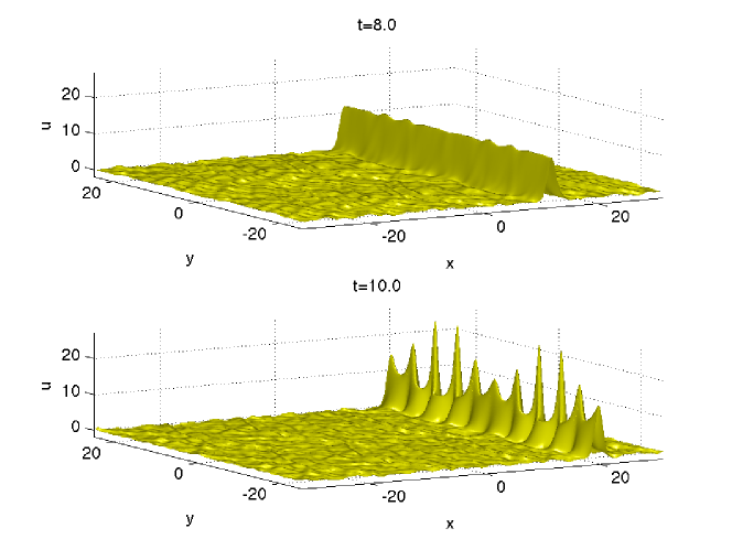
Figure 13. Solution to the KP I equation for initial data given by the KdV soliton $u_{sol}(x+2L_{x},0)$ plus perturbation $u_{p}=6(x-x_{1})\exp(-(x-x_{1})^{2})\left(\exp(-(y+L_{y}\pi/2)^{2})+\exp(-(y-L_{y}\pi/2)^{2})\right)$, $x_{1}=-L_{x}$ and the KdV soliton as in Fig. 12 ($L_{x}=8$) above and $L_{x}=10$ below.

Haragus and Pego [42] showed that the Zaitsev solution is an attractor for periodic (in $y$) perturbations of the line soliton. As we will illustrate below, the Zaitsev solution itself is unstable against periodic perturbations. To check the results of [42] one has to consider small periodic perturbations which travel with the wave. Above we do not have this restriction and find typically the formation of lumps that travel at higher speeds than the perturbed solution, thus violating the traveling wave condition. To get closer to the situation in [42], we consider initial data for the exact KdV soliton and a small perturbation given by the Zaitsev solution $u_{Zait}$ (25) of the form $u_{0}(x)=u_{sol}(x+L_{x},0)+0.1u_{Zait}(x+L_{x},y,0)$ with $\alpha=1$, $\beta=0.5$, $L_{x}=10$, $L_{y}=5/\delta$. The relative mass conservation $\Delta$ is of the order $10^{-7}$ and smaller until the lumps appear, and decreases then to $10^{-2}$. As can be seen in Fig. 14, the perturbation and the soliton essentially travel at the same speed for some time. One finds that the solution oscillates in this phase between the soliton and presumably the Zaitsev solution, until the instability against lump formation sets in.

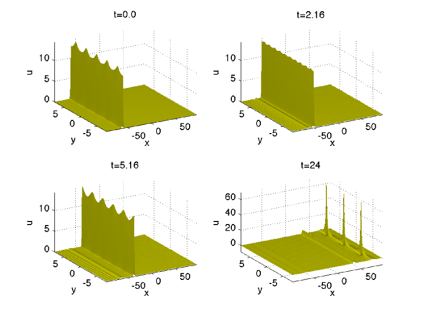
Figure 14. Solution to the KP I equation for initial data given by the KdV soliton plus perturbation given by the Zaitsev solution, $u_{0}=u_{sol}(x+L_{x},0)+0.1u_{Zait}(x+L_{x},y,0)$, $\alpha=1$, $\beta=0.5$, $L_{x}=10$, $L_{y}=5/\delta$ for various values of $t$.

These oscillations of the traveling wave profile between soliton and Zaitsev solution is even more visible if one studies the maximal amplitude of the solution in Fig. 14 in dependence of time as shown in Fig. 15. Three maxima can be recognized before the onset of lump formation. A similar behavior will be seen in the next subsection for a perturbation of the Zaitsev solution. In contrast to the situation shown in Fig. 13 the solution here does not change if a larger $L_{x}$ is chosen. The lump formation starts at roughly the same time as before.

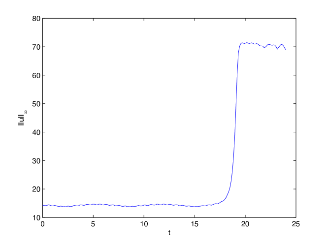
Figure 15. $L^{\infty}$-norm of the solution to the KP I equation of Fig. 14.

3.4. Perturbations of the Zaitsev solution

The KP I equation admits solutions that are exponentially localized in one spatial direction and periodic in the other. The simplest such solution (25) was found by Zaitsev [128]. The solution was generalized in [113]. We consider perturbations of the form $u_{p}=6(x+L_{x}/2)\exp(-(x+L_{x}/2)^{2}-y^{2})$ which satisfy the constraint (2.1). For the numerical experiments we choose $\alpha=1$, $\beta=0.5$, $L_{x}=10$, $L_{y}=5/\delta$, $N_{x}=2^{9}$, $N_{y}=2^{8}$, $N_{t}=10000$. With these settings we obtain a numerical mass conservation $\Delta<10^{-5}$. Notice that the unperturbed Zaitsev solution can be numerically propagated with the same precision as the line soliton, see [70].

For initial data given by the Zaitsev solution centered at $-L_{x}/2$ plus $u_{p}=6(x+L_{x}/2)\exp(-(x+L_{x}/2)^{2}-y^{2})$, we find the behavior shown in Fig. 16. One can see that the initial perturbation develops into a lump traveling faster than the remaining Zaitsev solution. The latter develops in the following further lumps in a similar way as the perturbed KdV soliton.

Figure 16. Solution to the KP I equation for initial data given by the Zaitsev solution $u_{Zait}(x+L_{x}/2,y,0)$ plus a perturbation $u_{p}=6(x+L_{x}/2)\exp(-(x+L_{x}/2)^{2}-y^{2})$ for various values of $t$.

Thus it appears that the Zaitsev solution is unstable as the line soliton against the formation of lumps. The precise pattern of the lumps depends on the initial perturbation. In Fig. 17 the same initial condition as in Fig. 16 is considered, this time however with a change in sign in the perturbation. The initial perturbation develops two lumps with further lumps forming at later times.

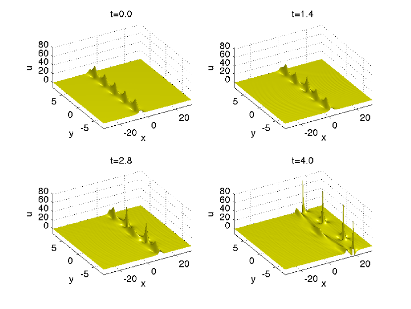
Figure 17. Solution to the KP I equation for initial data given by the Zaitsev solution $u_{Zait}(x+L_{x}/2,y,0)$ plus a perturbation $u_{p}=-6(x+L_{x}/2)\exp(-(x+L_{x}/2)^{2}-y^{2})$ for various values of $t$.

Notice that the Zaitsev solution is in some sense more unstable than the line soliton. First the amplitudes of the considered perturbations are a factor of 10 smaller than the amplitudes of the solution, and still the decay to lumps is almost immediate. More importantly the Zaitsev solution is also unstable against a displaced perturbation ($u_{p}=6x\exp(-x^{2}-y^{2})$) as can be seen in Fig. 18. As in Fig. 11 for the perturbed KdV soliton, the initial perturbation develops dispersive oscillations and tails, but the former almost immediately destroy the Zaitsev solution and leads to the formation of lumps, in contrast to the situation for the KdV soliton.

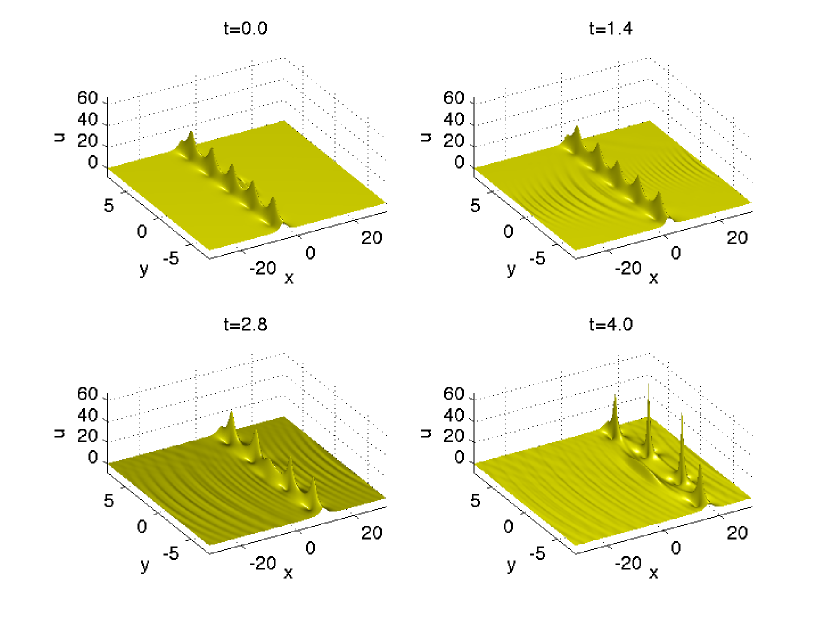
Figure 18. Solution to the KP I equation for initial data given by the Zaitsev solution plus a perturbation $u_{p}=6x\exp(-x^{2}-y^{2})$ for various values of $t$.

The Zaitsev solution also appears to be unstable against lump formation for perturbations with the same period in $y$. In Fig. 19 we show the time evolution of initial data from the Zaitsev solution as before, but with an amplitude multiplied by a factor of $1.1$. This corresponds to a small perturbation of exactly the same period as the Zaitsev solution.

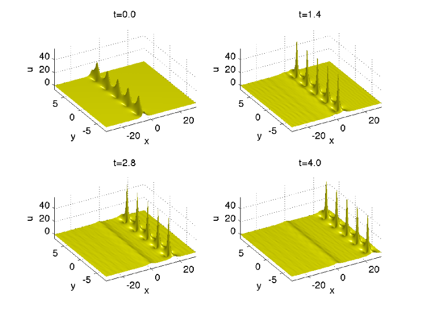
Figure 19. Solution to the KP I equation for initial data given by the Zaitsev solution plus a perturbation with the same period in $y$, $u_{0}(x)=1.1u_{Zait}(x+L_{x}/2,y,0)$ for various values of $t$.

It can be seen that each of the maxima of the initial data develops a lump-like structure. If we neglect the precise form of a multi-lump solution and just subtract a single lump at each of the final peaks in Fig. 19, we obtain Fig. 20. This suggests that the formed peaks will in fact develop asymptotically into a periodic array of lumps.

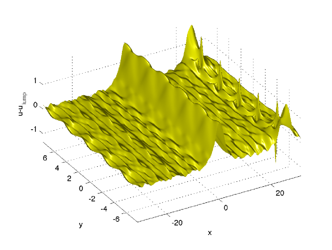
Figure 20. Difference of the solution to the KP I equation in Fig. 19 for $t=4$ and five lump solutions fitted at the peaks.

This is however only the case if the Zaitsev solution is multiplied with a factor greater than 1, i.e., if the humps are enlarged as above. In this case they seem to evolve into lumps. If instead the Zaitsev solution is multiplied by a factor smaller than 1, e.g. $0.9$, one gets for the time evolution of such data Fig. 21. The computation is carried out for $L_{x}=30$, $L_{y}=2.5$ with $N_{x}=2^{11}$, $N_{y}=2^{9}$ and $N_{t}=20000$ time steps to yield a $\Delta\sim 3*10^{-4}$. In this case one again observes oscillations between the Zaitsev solution and presumably the KdV soliton, until finally lump formation sets in.

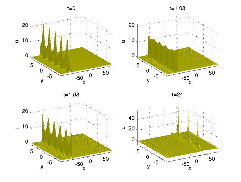
Figure 21. Solution to the KP I equation for initial data given by the Zaitsev solution plus a perturbation with the same period in $y$, $u_{0}(x)=0.9u_{Zait}(x+L_{x}/2,y,0)$ for various values of $t$.

In Fig. 22 it can be seen that this oscillatory phase can be quite long until lump formation starts. It appears that this oscillatory state is thus meta-stable in some sense, and the pattern does not change within the given precision if the code is run with $N_{t}=30000$.

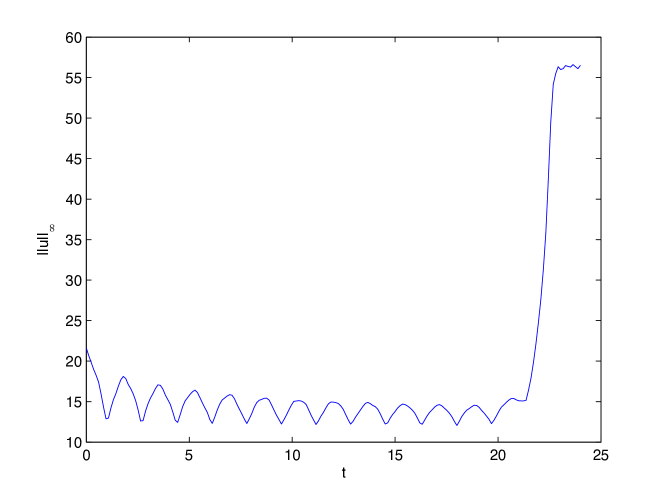
Figure 22. $L^{\infty}$-norm of the solution $u$ of Fig. 21 in dependence of time.

The mechanism of the final decay to lumps is not clear. If one runs the code with the same settings on a larger domain ($L_{x}=35$), lump formation sets in at roughly the same time. The same is true on a slightly reduced domain ($L_{x}=25$). Thus in contrast to the perturbation of the KdV soliton studied in Fig. 12, the proximity of the domain end in $x$-direction does not appear to be decisive. Instead it seems that numerical inaccuracies in the periodicity in $y$ trigger the lump formation. In fact if the same situation as in Fig. 21 is studied with a smaller $L_{y}=1.5$, the initial data show 3 maxima, which, however, develop into just two lumps as can be seen in Fig. 23. This indicates some symmetry breaking, presumably due to effects from the boundary of the computational domain in $y$-direction. The computation is carried out with $N_{x}=2^{11}$, $N_{y}=2^{8}$, $N_{t}=20000$ with a final $\Delta\sim 2*10^{-5}$. It does not change within the expected limit if a smaller resolution in space or time is chosen.

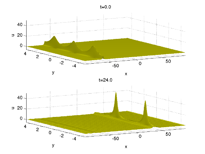
Figure 23. Solution to the KP I equation for the situation of Fig. 21 with a smaller $L_{y}=1.5$.

The $L^{\infty}$-norm of the solution in Fig. 23 can be seen in Fig. 24. In comparison to Fig. 22 it can be recognized that the lump formation starts at a slightly later time. Thus we cannot conclude what would happen if the same initial data would be treated on $\mathbb{R}\times\mathbb{T}$ instead of $\mathbb{T}^{2}$, but it seems that the instabilities here could be due to a sensitivity to inaccuracies in the $y$-periodicity.

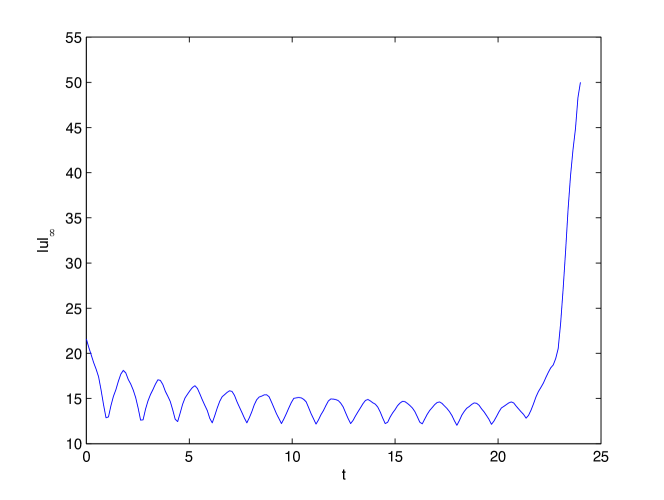
Figure 24. $L^{\infty}$-norm of the solution $u$ of Fig. 23 in dependence of time.

3.5. Numerical study of blowup in generalized KP equations

In this subsection we will study the time evolution of initial data $u_{0}(x)$ for the generalized KP equation (38). It is known [94] that the solution will blow up for initial data with negative energy for $p\geq 4/3$.

In the following we will consider the initial data

(47) $$u_{0}(x)=6\partial_{xx}\exp(-\alpha(x^{2}+y^{2})),\quad\alpha\in\mathbb{R}^{+}.$$

These data obviously satisfy the constraint (2.1).

For the supercritical $p=2$ we find that these data in fact imply a negative energy for $\alpha=1$. The computation is carried out with $L_{x}=5$, $L_{y}=2$, $N_{x}=2^{11}$, $N_{y}=2^{13}$ modes and $N_{t}=5000$ time steps. The code breaks at a finite time $t_{c}$ since the solution appears to develop a singularity. It is stopped once the quantity $\Delta$ measuring numerical mass conservation becomes larger than $10^{-4}$. It can be checked that the Fourier coefficients at this time ($t_{c}\sim 0.0473$ for the considered initial data) still decrease by 5 orders of magnitude. This implies that the solution is still accurate to better than plotting accuracy at this time.

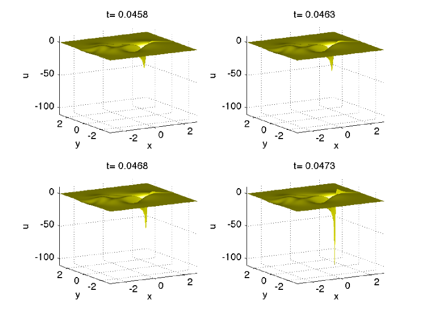
Figure 25. Solution to the generalized KP I equation ($p=2$) for the initial data $u_{0}(x,y)=6\partial_{xx}\exp(-(x^{2}+y^{2}))$ for various values of $t$.

It can be seen that the initial minimum develops apparently into a singularity. The precise formation of the latter is not isotropic in $x$ and $y$ as shown by the gradient of $u$ close to the critical time in Fig. 26. It can be seen that the $y$-derivative near the catastrophe is more than an order of magnitude bigger than the $x$-derivative. Thus it is foremost the $y$-derivative of the solution that diverges which then leads to a divergence of the solution itself. The much stronger gradients in $y$-direction are the reason why a higher resolution has to be chosen in $y$ than in $x$. With the used parameters we ensure essentially the same resolution in both spatial directions.

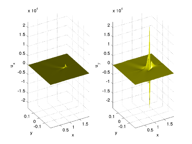
Figure 26. Gradient of the solution to the generalized KP I equation ($p=2$) for the initial data $u_{0}(x,y)=6\partial_{xx}\exp(-x^{2}-y^{2})$ for $t=0.0473$.

This behavior indicates that it is sensible to trace the time dependence of the $L^{\infty}$-norm of $u$ and the $L^{2}$-norm of $u_{y}$ which are shown in Fig. 27. Both norms diverge at the critical time. It can be seen that both norms are monotonically increasing, but that there is a steep divergence at the critical point. It is also obvious that the norm of $u_{y}$ diverges much more rapidly than $u$. From the obtained data one cannot decide the exact character of the divergence near the critical time (exponential, algebraic).

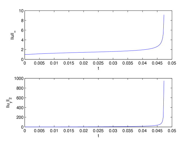
Figure 27. The $L^{\infty}$-norm of the solution to the KP I equation ($p=2$) for the initial data $u_{0}(x,y)=6\partial_{xx}\exp(-x^{2}-y^{2})$ and the $L^{2}$-norm of $u_{y}$ normalized to 1 for $t=0$ in dependence of time.

For the generalized KP II equation we find for the same $p$ and the same initial data that there is no indication for blowup. The time evolution of the solution can be seen in Fig. 28. It can be seen that the typical oscillations in $x$-direction due to the Airy term in the KP equation appear, see [68]. The algebraic fall off to infinity typical for KP solutions even for Schwartzian initial data is clearly visible in the form of tails to the left.

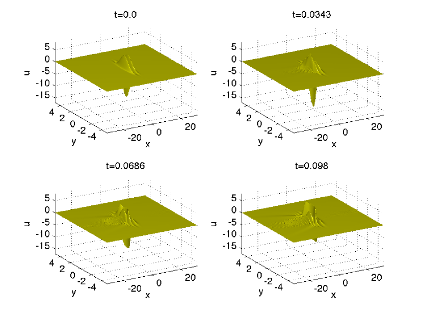
Figure 28. Solution to the generalized KP II equation ($p=2$) for the initial data $u_{0}(x,y)=6\partial_{xx}\exp(-x^{2}-y^{2})$ for various times.

In contrast to the KP I case, there is no indication for a blow up. In Fig. 29 the $L^{\infty}$-norm of $u$ and of the $L^{2}$-norm of $u_{y}$ are shown. The former seems to decrease since the negative hump is essentially radiated away to infinity via the tails or to lead to the dispersive oscillations. The $L^{2}$-norm of $u_{y}$ appears to approach slowly a finite asymptotic value.

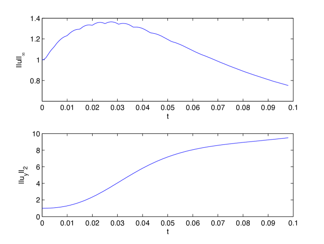
Figure 29. The $L^{\infty}$-norm of the solution to the generalized KP II equation ($p=2$) for the initial data $u_{0}(x,y)=6\partial_{xx}\exp(-x^{2}-y^{2})$ and the $L^{2}$-norm of $u_{y}$ normalized to 1 for $t=0$ in dependence of time.

For the standard KP I equation ($p=1$) similar initial data lead as expected to a regular solution as can be seen in Fig. 30. The energy for these initial data is positive. The solution just shows the characteristic oscillations and the tails. This computation and the ones below are carried out with $N_{x}=2^{10}$ and $N_{y}=2^{8}$ and $N_{t}=1000$ time steps. The Fourier coefficients decrease to $10^{-4}$ which ensures spatial resolution, and the relative mass conservation is numerically satisfied to better than $10^{-6}$. Thus with numerical precision we can exclude the formation of a singularity up the considered time $t=0.15$.

Figure 30. Solution to the KP I equation ($p=1$) for the initial data $u_{0}(x,y)=12\partial_{xx}\exp(-x^{2}-y^{2})$ for $t=0.15$.

The $L^{\infty}$-norm of $u$ and the $L^{2}$-norm of $u_{y}$ both decrease for large times. Thus there is no indication of the appearance of a singularity as expected.

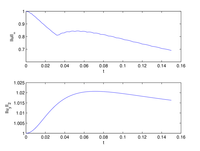
Figure 31. The $L^{\infty}$-norm of the solution to the KP I equation ($p=1$) for the initial data $u_{0}(x,y)=12\partial_{xx}\exp(-x^{2}-y^{2})$ and the $L^{2}$-norm of $u_{y}$ normalized to 1 for $t=0$ in dependence of time.

For the critical exponent $p=4/3$ we obtain for the initial data (47) with $\alpha=4$, which leads to a negative energy, the solution shown in Fig. 32.

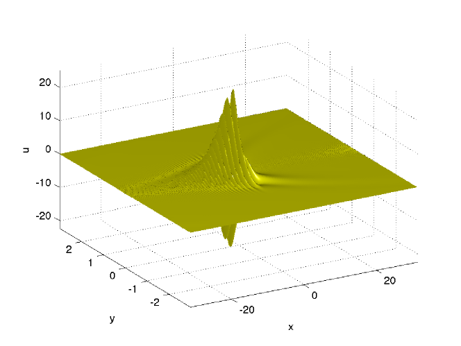
Figure 32. Solution to the generalized KP I equation with critical exponent $p=4/3$ for the initial data $u_{0}(x,y)=6\partial_{xx}\exp(-4(x^{2}+y^{2}))$ for $t=0.05$.

There is no indication of a divergence of the solution, and the $L^{\infty}$-norm of $u$ actually decreases as can be seen in Fig. 33. However the $L^{2}$-norm of $u_{y}$ seems to increase without bound in accordance with the theory. It appears that no blowup happens for finite times, but this can of course not be decided with numerical methods alone. We just did not see an indication of a blowup for even longer times.

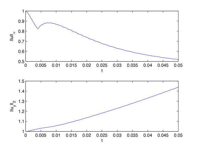
Figure 33. The $L^{\infty}$-norm of the solution to the generalized KP I equation with critical exponent $p=4/3$ for the initial data $u_{0}(x,y)=6\partial_{xx}\exp(-4(x^{2}+y^{2}))$ and the $L^{2}$-norm of $u_{y}$ normalized to 1 for $t=0$ in dependence of time.

Acknowledgements.

We thank M. Haragus for useful discussions and hints. The second Author thanks L. Molinet and N. Tzvetkov for useful suggestions and for a lengthy and fruitful joint research on KP equations. This work has been supported in part by the project FroM-PDE funded by the European Research Council through the Advanced Investigator Grant Scheme, the Conseil Régional de Bourgogne via a FABER grant, the ANR via the program ANR-09-BLAN-0117-01 and the Wolfgang Pauli Institute in Vienna.

References

- [1] M. J. Ablowitz and P. A. Clarkson, Solitons, nonlinear evolution equations and inverse scattering, Cambridge Univ. Press, Cambridge (1991).
- [2] M. J. Ablowitz and A. Fokas, On the inverse scattering and direct linearizing transforms for the Kadomtsev-Petviashvili equation, Physics Letters A, 94, no. 2 (1983), 67-70.
- [3] M. J. Ablowitz and H. Segur, On the evolution of packets of water waves, J. Fluid Mech. 92 1979, 691-715.
- [4] M. J. Ablowitz, J. Villarroel, The Cauchy problem for the Kadomtsev-Petviashvili II equation with with nondecaying data along a line, Studies Appl. Math 109 (2002), 151-162.
- [5] M. J. Ablowitz, J. Villarroel, The Cauchy problem for the Kadomtsev-Petviashvili II equation with data that do not decay along a line, Nonlinearity 17 (2004), 1843-1866.
- [6] L. A. Abramyan and Y. A. Stepanyants, The structure of two-dimensional solitons in media with anomalously small dispersion, Sov. Phys JETP, 61, no. 5 (1985), 963-966.
- [7] J. C. Alexander, R. L. Pego, and R. L. Sachs, On the transverse instability of solitary waves in the Kadomtsev-Petviashvili equation, Phys. Lett. A 226 (1997), 187–192.
- [8] D. Alterman and J. Rauch, The linear diffractive pulse equation, Methods and Applications of Analysis, 7, no. 2 (1999), 263-274.
- [9] M. Ben-Artzi, and J.-C. Saut, Uniform decay estimates for a class of oscillatory integrals and applications Differential Integral Equations 12, no. 2 (1999), 137–145.
- [10] T.B. Benjamin, J.L. Bona and J.J. Mahony, Models equations for long waves in nonlinear dispersive systems, Phil.Trans. Roy. Soc. London Series A Mathematical and Physical Sciences 272 (1972), 47-78.
- [11] Y. Ben-Youssef and D. Lannes, The long wave limit for a general class of 2D quasilinear hyperbolic problems, Comm. Partial Diff. Eq. 27 n 5-6 (2002), 979-1020.
- [12] O. V. Besov, V. P. Il’in and S. M. Nikolskii, Integral representations of functions and imbedding theorems, Vol. I, J. Wiley, New York, 1978.
- [13] F. Béthuel, P. Gravejat and J.-C. Saut, On the KP I transonic limit of two-dimensional Gross-Pitaevskii travelling waves, Dyn. Partial Differ. Equ. 5, no. 3 (2008), 241–280.
- [14] M. Boiti, F. Pempinelli, and A. Pogrebkov, Properties of solutions of the Kadomtsev-Petviashvili I equation, J. Math. Phys. 35 (1994), issue 9, 4683–4718.
- [15] J. L. Bona and Y. Liu, Instability of solitary- wave solutions of the 3-dimensional Kadomtsev-Petviashvili equation, Advances Diff. Eq. 7, no. 1 (2002), 1-23.
- [16] J. L. Bona, Y. Liu and M. Tom, The Cauchy problem and stability of solitary wave solutions for RLW-KP type equations, J. Differential Equations 185, no. 2 (2002), 437-482.
- [17] J. L. Bona, W. G. Pritchard and L.R. Scott, A comparison of solutions of two model equations for long waves, Lect. Appl. Math. 20 (1983), 235-267.
- [18] A. de Bouard and Y. Martel, Nonexistence of -compact solutions of the Kadomtsev-Petviashvili II equation, Math. Annalen. 328 (2004), 525–544.
- [19] A. de Bouard and J.-C. Saut, Solitary waves of the generalized KP equations, Ann. IHP Analyse Non Linéaire 14, 2 (1997), 211-236.
- [20] A. de Bouard and J.-C. Saut, Symmetry and decay of the generalized Kadomtsev-Petviashvili solitary waves SIAM J. Math. Anal. 28, 5 (1997), 104-1085
- [21] A. de Bouard and J.-C. Saut, Remarks on the stability of the generalized Kadomtsev-Petviashvili solitary waves, in Mathematical Problems in The Theory of Water Waves, F. Dias J.-M. Ghidaglia and J.-C. Saut (Editors), Contemporary Mathematics 200 AMS 1996, 75-84.
- [22] J. Bourgain,On the Cauchy problem for the Kadomtsev-Petviashvili equation, Geom. Funct. Anal. 3 (1993), no.4, 315–341.
- [23] D. Chiron and F. Rousset, The KdV/KP limit of the Nonlinear Schrödinger equation, SIAM J. Math.Anal. 42, 1 (2010), 64-96.
- [24] J. Colliander, C. Kenig, and G. Staffilani, Low regularity solutions for the Kadomtsev-Petviashvili I equation, Geom. Funct. Anal. 13 (2003), no.4, 737–794.
- [25] S. M. Cox and P. C. Matthews, Exponential time differencing for stiff systems, J. Comput. Phys., 176 (2) (2002), pp. 430-455.
- [26] V. S. Druyma, On the analytical solution of the two-dimensional Korteweg-de Vries equation, Sov. Phys. JETP Letters, 19 (1974) 753-757.
- [27] A. S. Fokas , Lax pairs : a novel type of separability, Inverse Problems 25 (2009), 1-44.
- [28] A. S. Fokas and L. Y. Sung, On the solvability of the N-wave, Davey-Stewartson and Kadomtsev-Petviashvili equations, Inverse Problems 8 (1992), 673–708.
- [29] A.S. Fokas and A.K. Pogrebkov, Inverse scattering transform for the KP I equation on the background of a one- line soliton, Nonlinearity 16 (2003), 771-783.
- [30] A. S. Fokas and L. Y. Sung, The inverse spectral method for the KP I equation without the zero mass constraint, Math. Proc. Camb. Phil. Soc. 125 (1999), 113-138.
- [31] T. Gallay and G. Schneider, KP description of unidirectional long waves. The model case, Proc. Roy. Soc. Edinburgh Ser. A 131 n 4 (2001), 885-898.
- [32] J. Ginibre, Le problème de Cauchy pour des EDP semi linéaires périodiques en variables d’espace, Sém. N. Bourbaki, (1994-1995), exp. No. 706, 163-187.
- [33] Ph Gravejat, Asymptotics of the solitary waves for the generalised Kadomtsev-Petviashvili equations, Discrete Contin. Dynam. Systems, 21, no.3 (2008), 835-882;
- [34] M.D. Groves, M. Haragus and S.M. Sun, A dimension breaking phenomenon in the theory of steady gravity-capillary water waves, Phil.Trans. Roy. Soc. Lond. A 360 (2002), 2189-2243.
- [35] A. Grünrock, On the Cauchy problem for generalized Kadomtsev-Petviashvili (KP II) equations, Electronic Journal Differential Equations 82 (2009), 1-9.
- [36] A. Grünrock, M. Panthee and J. Drumond Silva, On KP II equations on cylinders, Ann. IHP Analyse Non Linéaire 26 6 (2009), 2335-2358.
- [37] Z. Guo, L. Peng and B. Wang, On the local regularity of the KP I equation in anisotropic Sobolev spaces, J. Math. Pures Appliquées, 94 (2010), 414-432.
- [38] M. Hadac, Well-posedness for the Kadomtsev (KP II) equation and generalizations, Trans. Amer. Math. Soc. 360 (2008), 6555-6572.
- [39] M. Hadac, Well-posedness for the Kadomtsev-Petviashvili II equation and generalisations, Trans. Amer. Math. Soc. 360 no. 12, (2008), 6555–6572.
- [40] M. Hadac, S. Herr and H. Koch, Well-posedness and scattering for the KP II equation in a critical space, Ann. IHP Analyse Non Linéaire 26, 3 (2009), 917-941.
- [41] F. Hamidouche, Y. Mammeri and S. Mefire, Numerical study of the solutions of the 3D generalized KadomtsevPetvisahvili equations for long times, CICP Commun. Comput. Phys. 6 no. 5 (2009), 1022-1062.
- [42] M. Haragus and R.L. Pego, Travelling waves of the KP equations with transverse modulations C. R. Acad. Sci. Paris, Vol. 328, Série I (1999), 227-232.
- [43] N. Hayashi, P. Naumkin and J.-C. Saut, Asymptotics for larg e time of global solutions to the generalized Kadomtsev-Petviashvili equation, Comm. Math. Phys. 201 (1999), 577-590.
- [44] M. Hochbruck and A. Ostermann, Exponential integrators, Acta Numerica 19, 209-286 (2010).
- [45] G. Huang, V. A. Makarov, and M. G. Velarde, Two-dimensional solitons in Bose-Einstein condensates with a disk-shaped trap, Phys. Rev. A 67 (2003), 23604–23616.
- [46] E. Infeld, A. Senatorski, and A. A. Skorupski, Numerical simulations of Kadomtsev-Petviashvili soliton interactions, Phys. Rev. E 51 (1995), 3183- 3191.
- [47] E. Infeld, A. A. Skorupski, and G. Rowlands, Instabilities and oscillations of one- and two-dimensional Kadomtsev-Petviashvili waves and solitons. II. Linear to nonlinear analysis. R. Soc. Lond. Proc. Ser. A (Math. Phys. Eng. Sci.) 458 (2002), no. 2021, 1231–1244.
- [48] A. Ionescu and C. Kenig, Local and global well-posedness of periodic KP I eqations, Annals of Math. Studies 163 (2007), 181-211.
- [49] A. D. Ionescu, C. Kenig and D. Tataru, Global well-posedness of the initial value problem for the KP I equation in the energy space, Invent. Math. 173 2 (2008), 265-304.
- [50] R.J. Iório Jr. and W.V.L.Nunes, On equations of KP-type, Proc. Roy. Soc. Edinburgh 128 (1998), 725-743.
- [51] P. Isaza, J. Lopez and J. Mejia, Cauchy problem for the fifth order Kadomtsev-Petviashvili (KP II) equation, Comm. on Pure and Appl. Anal. 5, no. 4 ((2006), 887-905.
- [52] P. Isaza, J. Lopez and J. Mejia, The Cauchy problem for the Kadomsteev-Petviashvili (KP II) equation in thee space dimensions, Comm. Partial Diff. Eq. 32 (2007), 611-641.
- [53] P. Isaza and J. Mejia, Local and global Cauchy problems for the Kadomtsev-Petviashvili (KP-II) equation in Sobolev spaces of negative indices, Comm. PDE 26 (2001), 1027-1057.
- [54] P. Isaza and J. Mejia, A smoothing effect and polynomial growth of the Sobolev norms for the KP II equation, J. Diff. Equations 220 (2006), 1-17.
- [55] R. S. Johnson, The classical problem of water waves: a reservoir of integrable and nearly integrable equations, J. Nonl. Math. Phys. 10 (2003) 72–92.
- [56] C. A. Jones and P. H. Roberts, Motions in a Bose condensate, IV: Axisymmetric solitary waves, J. Phys. A Math. Gen. 15 (1982), 2599–2619.
- [57] B. B. Kadomtsev and V. I. Petviashvili, On the stability of solitary waves in weakly dispersing media, Sov. Phys. Dokl. 15 (1970), 539–541.
- [58] V. I. Karpman and V. YU. Belashov, Dynamics of two-dimensional solitons in weakly dispersing media, Phys. Rev. Lett. A 154 (1991), 131-139.
- [59] V. I. Karpman and V. YU. Belashov, Evolution of three-dimensional pulses in weakly dispersive media, Phys. Rev. Lett. A 154 (1991), 140-144.
- [60] T. Kato, On the Cauchy problem for the (generalized) Korteweg - de Vries equations, Advances in Mathematics, Supplementary Studies, Stud. Appl. Math. 8 (1983), 93-128.
- [61] D. Kaya and E. M. Salah, Numerical soliton-like solutions of the potential Kadomtsev-Petviashvili equation by the decomposition method, Phys. Lett. A 320 (2003), no. 2-3, 192–199.
- [62] C. Kenig, On the local and global well-posedness for the KP-I equation, Annales IHP Analyse Non Linéaire 21 (2004), 827-838.
- [63] C. Kenig Recent progress on the global well-posedness of the Kadomtsev-Petviashvili I equation, Proc. Conf. in Honour of C. Segovia, Birkhaüser.
- [64] C.Kenig and Y. Martel, Global well-posedness in the energy space for a modified KP II equation via the Miura transform, TAMS 358 (2006), 2447-2488.
- [65] C. Kenig and S. Ziegler Local well-posedness for modified Kadomtsev-Petviashvii equations , Diff. and Int. Equations 18 (2005), 111-146.
- [66] C. Kenig and S. Ziegler Maximal function estimates with applications to a modified KP equation, Comm. Pure Appl. Analysis 4 n 1 (2005), 45-91.
- [67] C. Klein, Fourth order time-stepping for low dispersion Korteweg-de Vries and nonlinear Schrödinger equation, ETNA 29 (2008), 116-135 .
- [68] C. Klein, C. Sparber and P. Markowich , Numerical study of oscillatory regimes in the Kadomtsev-Petviashvili equation, J. Nonl. Sci. 17, no. 5 (2007), 429-470.
- [69] C. Klein and C. Sparber, Numerical simulation of generalized KP type equations with small dispersion, in ‘Recent Progress in Scientific Computing’, ed. by W.-B. Liu, Michael Ng and Zhong-Ci Shi, Science Press (Beijing) (2007).
- [70] C. Klein and K. Roidot, Fourth order time-stepping for small dispersion Kadomtsev-Petviashvili and Davey-Stewartson equations, preprint (2010).
- [71] H. Koch and N. Tzvetkov, On finite energy solutions of the KP I equation, Math. Z. 258, no. 1 (2008), 55-68.
- [72] B. Kojok, Sharp well-posedness for the Kadomtsev-Petviashvili-Burgers (KP -B-II) equation in , J. Diff. Equations 242 no.2 (2007), 211-247.
- [73] I. M. Krichever, The averaging method for two-dimensional integrable equations, Funktsional. Anal. i Prilozhen. 22 (1988), no. 3, 37–52; translation in Funct. Anal. Appl. 22 (1989), no. 3, 200–213.
- [74] D Lannes, Consistency of the KP approximation, Discrete Cont. Dyn. Syst. (2003) Suppl. 517-525.
- [75] D. Lannes and J.-.C. Saut, Weakly transverse Boussinesq systems and the KP approximation, Nonlinearity 19 (2006), 2853-2875.
- [76] P. D. Lax and C. D. Levermore, The small dispersion limit of the Korteweg de Vries equation I,II,III, Comm. Pure Appl. Math. 36 (1983), 253–290, 571–593, 809–830.
- [77] J. L. Levandovsky, Gain of regularity for the KP II equation, Indiana Math J. 49, no. 1 (2000), 353-403
- [78] J. L. Levandovsky, M. Sepúlveda and O.Vera Villagrán, Gain of regularity for the KP I equation, J. Diff. Eq. 245 (2008), 762-808.
- [79] C. D. Levermore, The hyperbolic nature of the zero dispersion KdV limit, Comm. Part. Diff. Equ. 13 (1988), no. 4, 495–514.
- [80] J. Li and J. Xiao Well-posedness of the fifth order KP-I equation in anisotropic spaces with nonnegative indices, J. Math. Pures Appl. 94 (2010), 414-432.
- [81] Yue Liu, Blow-up and instability of solitary- wave solutions to a generalized Kadomtsev-Petviashvili equation, TAMS 353 (2001), 191-208.
- [82] Yue Liu, Strong instablity of solitary- wave solutions to a Kadomtsev-Petviashvili in three dimensions, J. Diff. Eq. 180 (2002), 153-170.
- [83] Yue Liu and X. P. Wang, Nonlinear stability of solitary waves of generalized Kadomtsev-Petviashvili equations, Comm. Math. Phys. 183, no. 2 (1997), 253-266.
- [84] Manakov S.V., Zakharov V.E., Bordag L.A. and Matveev V.B., Two-dimensional solitons of the Kadomtsev-Petviashvili equation and their interaction, Phys. Lett. A 63, 205-206 (1977).
- [85] D. W. McLaughlin and J. A. Strain, Computing the weak limit of KdV, Comm. Pure Appl. Math. 47 (1994), no. 10, 1319–1364.
- [86] Y. Mammeri, Comparaison entre modèles d’ondes de surface en dimension 2, ESAIM M2AN 41, no.3 (2007), 513-542.
- [87] B. Merlet and L. Paumond, A initial boundary-value problem for the KP II equation on a strip and on the half plane, Differential and Integral Equations 18 n 7 (2005), 813-839.
- [88] B. Minchev and W. Wright, A review of exponential integrators for first order semi-linear problems, Technical Report 2, The Norwegian University of Science and Technology (2005).
- [89] T. Mizomachi and N. Tzvetkov, Stability of the line soliton of the KP II equation under periodic transverse perturbations, arXiv: 1008.0812v1. .
- [90] L. Molinet, On the asymptotic behavior of solutions to the (generalized) Kadomtsev-Petviashvili-Burgers equation, J. Diff. Eq. 152 (1999), 30-74.
- [91] L. Molinet and F. Ribaud, The global Cauchy problem in Bourgain type spaces for a dispersive-dissipative semilinear equation, SIAM J. Math. Anal. 33 no. 6 (2002), 1269-1296.
- [92] L. Molinet, J. C. Saut, and N. Tzvetkov, Well-posedness and ill-posedness results for the Kadomtsev-Petviashvili-I equation, Duke Math. J. 115 no. 2 (2002), 353-384.
- [93] L. Molinet, J. C. Saut, and N. Tzvetkov, Remarks on the mass constraint for KP type equations, SIAM J. Math. Anal. 39, no.2 (2007), 627-641.
- [94] L. Molinet, J.C. Saut and N. Tzvetkov, Global well-posedness for the KP-I equation, Math. Annalen 324, (2002), pp. 255-275. Correction : Math. Ann. 328 (2004), 707–710.
- [95] L. Molinet, J.C. Saut and N. Tzvetkov,Global well-posedness for the KP-I equation on the background of a non localized solution, Commun. Math. Phys. 272 (2007), 775-810.
- [96] L. Molinet, J.C. Saut and N. Tzvetkov,Global well-posedness for the KP-II equation on the background of a non localized solution, preprint.
- [97] S. Novikov, S. V. Manakov, L. P. Pitaevskii, and V. E. Zakharov, Theory of Solitons: The Inverse Scattering Method Springer Monographs in Contemporary Mathematics, Springer 1984.
- [98] M. Panthee, Unique continuation property for the Kadomtsev-Petviashvili (KP-II) equation, Electronic J. Dif. Eq. 59 (2005), 1-12.
- [99] L. Paumond A rigorous link between KP and a Benney-Luke equation, Diff. Integral Equations 16 n 9 (2003), 1039-1064.
- [100] L. Redekopp, Similarity solutions of some two-dimensional nonlocal wave evolution equations, Stud. Appl. Math. 63 (1980), 185-207.
- [101] F. Rousset and N. Tzvetkov, Transverse nonlinear instability for two-dimensional dispersive models, Annales IHP ANL 26 (2009), 477-496.
- [102] J. Satsuma, N-soliton of the two-dimensional Korteweg-de Vries equation, J. Phys. Soc. Japan, 40 (1976), 286-290.
- [103] J. -C. Saut, Remarks on the generalized Kadomtsev-Petviashvili equations, Indiana Univ. Math. J., 42 (1993), 1011-1026.
- [104] J. -C. Saut, Recent results on the generalized Kadomtsev-Petviashvili equations, Acta Appl. Math. 39 (1995) , 477-487.
- [105] J. -C.- Saut and N. Tzvetkov, On the periodic KP-I type equations, Comm. Math. Phys. 221 (2001), 451-476.
- [106] J.- C.- Saut and N. Tzvetkov, The Cauchy problem for higher order KP equations, J. Diff. Eq. 153 1 (1999), 196-222.
- [107] J.- C.- Saut and N. Tzvetkov, The Cauchy problem for the fifth order KP equation, J. Math. Pures Appl. 79 4 (2000), 307-338.
- [108] J.- C. Saut and N. Tzvetkov, Global well-posedness for the KP-BBM equations, AMRX Appl. Math. Res. Express, 1 (2004), pp. 1–16.
- [109] M. Schwarz, Jr. Periodic solutions of Kadomtsev-Petviashvili, Adv. Math. 66 (1987) 217-233.
- [110] A. Senatorski and E. Infeld, Simulations of Two-Dimensional Kadomtsev-Petviashvili Soliton Dynamics in Three-Dimensional Space, Phys. Rev. Lett. 77 (1996), 2855- 2858.
- [111] C. Sulem and P.-L. Sulem, The nonlinear Schrödinger equation, Springer-Verlag, Applied Mathematical Sciences 139 New York, Berlin 1999.
- [112] Li-Yeng Sung, Square integrability and uniqueness of the solutions of the Kadomtsev-Petviashvili-I equation, Mathematical Physics, Analysis and Geometry 2 (1999), 1-24.
- [113] M. Tajeri and Y. Murakami, J. Phys. Soc. Japan 58 (1989) 3029.
- [114] M. Tajeri, Y. Murakami, The periodic soliton resonance : solutions of the Kadomtsev-Petviashvili equation with positive dispersion, Phys. Lett. A 143 (1990) 217-220.
- [115] H. Takaoka, Global well-posedness for the Kadomtsev-Petviashvili II equation, Discrete Contin. Dynam. Systems, 6 (2000), 483–499.
- [116] H. Takaoka, N. Tzvetkov, On the local regularity of Kadomtsev-Petviashvili-II equation, IMRN 8 (2001), 77-114.
- [117] H. Takaoka, Global well-posedness for the Kadomtsev-Petviashvili II equation, Discrete Contin. Dynam. Systems 6 (2000), 483–499.
- [118] H. Takaoka and N. Tzvetkov, On the local regularity of the Kadomtsev- Petviashvili-II equation, Internat. Math. Res. Notices 2001 (2001), no. 2, 77–114.
- [119] M. M. Tom, On a generalized Kadomtsev-Petviashvili equation, Contemporary Mathematics AMS, 200 (1996), 193-210.
- [120] S. Turitsyn and G. Falkovitch, Stability of magneto-elastic solitons and self-focusing of sound in antiferromagnets, Soviet Phys. JETP 62 (1985), 146–152.
- [121] N. Tzvetkov, On the Cauchy problem for Kadomtsev-Petviashvili equation. Comm. Partial Diff. Equations 24 no.7, 8 (1999), 1367–1397.
- [122] N. Tzvetkov, Global low regularity solutions for Kadomtsev-Petviashvili equation, Diff. Int. Eq. 13 (2000), 1289-1320.
- [123] N. Tzvetkov, it Long time bounds for the periodic KP II equation, IMRN 46 (2004), 2485-2496.
- [124] S. Ukaï, Local solutions of the Kadomtsev-Petviashvili equation, J. Fac. Sci. Univ. Tokyo Sect. IA Math. 36 (1989), 193-209.
- [125] X. P. Wang, M. Ablowitz, and H. Segur, Wave collapse and instability of solitary waves of a generalized Kadomtsev-Petviashvili equation, Physica D 78 (1994), 241–265.
- [126] A. Wazwaz, A computational approach to soliton solutions of the Kadomtsev-Petviashvili equation, Appl. Math. Comput. 123 (2001), no. 2, 205–217.
- [127] M.V. Wickerhauser, Inverse scattering for the heat equation and evolutions in variables, Comm. Math. Phys. 108 (1987), 67-89.
- [128] A.A. Zaitsev, Formation of stationary waves by superposition of solitons, Sov. Phys. Dokl. 28 (9) (1983), 720-722.
- [129] V.E. Zakharov, Instability and nonlinear oscillations of solitons, JETP Lett. 22 (1975), 172-173.
- [130] V.E. Zakharov, Weakly nonlinear waves on the surface of an ideal finite depth fluid, Amer. Math. Soc. Transl. 182 (2) (1998), 167-197.
- [131] V. Zakharov, E. Schulman, Degenerative dispersion laws, motion invariants and kinetic equations, Physica D 1 (1980), 192-202.
- [132] X. Zhou, Inverse scattering transform for the time dependent Schrödinger equation with applications to the KP-I equation, Comm. Math. Phys. 128 (1990) 551-564.