On the Convexity of Latent Social Network Inference

Abstract

In many real-world scenarios, it is nearly impossible to collect explicit social network data. In such cases, whole networks must be inferred from underlying observations. Here, we formulate the problem of inferring latent social networks based on network diffusion or disease propagation data. We consider contagions propagating over the edges of an unobserved social network, where we only observe the times when nodes became infected, but not who infected them. Given such node infection times, we then identify the optimal network that best explains the observed data. We present a maximum likelihood approach based on convex programming with a $l_{1}$-like penalty term that encourages sparsity. Experiments on real and synthetic data reveal that our method near-perfectly recovers the underlying network structure as well as the parameters of the contagion propagation model. Moreover, our approach scales well as it can infer optimal networks of thousands of nodes in a matter of minutes.

1 Introduction

Social network analysis has traditionally relied on self-reported data collected via interviews and questionnaires [27]. As collecting such data is tedious and expensive, traditional social network studies typically involved a very limited number of people (usually less than 100). The emergence of large scale social computing applications has made massive social network data [16] available, but there are important settings where network data is hard to obtain and thus the whole network must thus be inferred from the data. For example, populations, like drug injection users or men who have sex with men, are “hidden” or “hard-to-reach”. Collecting social networks of such populations is near impossible, and thus whole networks have to be inferred from the observational data.

Even though inferring social networks has been attempted in the past, it usually assumes that the pairwise interaction data is already available  [5]. In this case, the problem of network inference reduces to deciding whether to include the interaction between a pair of nodes as an edge in the underlying network. For example, inferring networks from pairwise interactions of cell-phone call [5] or email [4, 13] records simply reduces down to selecting the right threshold $\tau$ such that an edge $(u,v)$ is included in the network if $u$ and $v$ interacted more than $\tau$ times in the dataset. Similarly, inferring networks of interactions between proteins in a cell usually reduces to determining the right threshold [9, 20].

We address the problem of inferring the structure of unobserved social networks in a much more ambitious setting. We consider a diffusion process where a contagion (e.g., disease, information, product adoption) spreads over the edges of the network, and all that we observe are the infection times of nodes, but not who infected whom i.e. we do not observe the edges over which the contagion spread. The goal then is to reconstruct the underlying social network along the edges of which the contagion diffused.

We think of a diffusion on a network as a process where neighboring nodes switch states from inactive to active. The network over which activations propagate is usually unknown and unobserved. Commonly, we only observe the times when particular nodes get “infected” but we do not observe who infected them. In case of information propagation, as bloggers discover new information, they write about it without explicitly citing the source [15]. Thus, we only observe the time when a blog gets “infected” but not where it got infected from. Similarly, in disease spreading, we observe people getting sick without usually knowing who infected them [26]. And, in a viral marketing setting, we observe people purchasing products or adopting particular behaviors without explicitly knowing who was the influencer that caused the adoption or the purchase [11]. Thus, the question is, if we assume that the network is static over time, is it possible to reconstruct the unobserved social network over which diffusions took place? What is the structure of such a network?

We develop convex programming based approach for inferring the latent social networks from diffusion data. We first formulate a generative probabilistic model of how, on a fixed hypothetical network, contagions spread through the network. We then write down the likelihood of observed diffusion data under a given network and diffusion model parameters. Through a series of steps we show how to obtain a convex program with a $l_{1}$-like penalty term that encourages sparsity. We evaluate our approach on synthetic as well as real-world email and viral marketing datasets. Experiments reveal that we can near-perfectly recover the underlying network structure as well as the parameters of the propagation model. Moreover, our approach scales well since we can infer optimal networks of a thousand nodes in a matter of minutes.

Further related work. There are several different lines of work connected to our research. First is the network structure learning for estimating the dependency structure of directed graphical models [7] and probabilistic relational models [7]. However, these formulations are often intractable and one has to reside to heuristic solutions. Recently, graphical Lasso methods [25, 21, 6, 19] for static sparse graph estimation and extensions to time evolving graphical models [1, 8, 22] have been proposed with lots of success. Our work here is similar in a sense that we “regress” the infection times of a target node on infection times of other nodes. Additionally, our work is also related to a link prediction problem [12, 23, 18, 24] but different in a sense that this line of work assumes that part of the network is already visible to us.

The work most closely related to ours, however, is  [10], which also infers networks through cascade data. The algorithm proposed (called NetInf) assumes that the weights of the edges in latent network are homogeneous, i.e. all connected nodes in the network infect/influence their neighbors with the same probability. When this assumption holds, the algorithm is very accurate and is computationally feasible, but here we remove this assumption in order to address a more general problem. Furthermore, where  [10] is an approximation algorithm, our approach guarantees optimality while easily handling networks with thousands of nodes.

2 Problem Formulation and the Proposed Method

We now define the problem of inferring a latent social networks based on network diffusion data, where we only observe identities of infected nodes. Thus, for each node we know the interval during which the node was infected, whereas the source of each node’s infection is unknown. We assume only that an infected node was previously infected by some other previously infected node to which it is connected in the latent social network (which we are trying to infer). Our methodology can handle a wide class of information diffusion and epidemic models, like the independent contagion model, the Susceptible–Infected (SI), Susceptible–Infected–Susceptible (SIS) or even the Susceptible–Infected–Recovered (SIR) model [2]. We show that calculating the maximum likelihood estimator (MLE) of the latent network (under any of the above diffusion models) is equivalent to a convex problem that can be efficiently solved.

Problem formulation: The cascade model. We start by first introducing the model of the diffusion process. As the contagion spreads through the network, it leaves a trace that we call a cascade. Assume a population of $N$ nodes, and let $A$ be the $N\times N$ weighted adjacency matrix of the network that is unobserved and that we aim to infer. Each entry $(i,j)$ of $A$ models the conditional probability of infection transmission:

$$A_{ij}=P(\mbox{node $i$ infects node $j$}\ |\ \mbox{node $i$ is infected}).$$

The temporal properties of most types of cascades, especially disease spread, are governed by a transmission (or incubation) period. The transmission time model $w(t)$ specifies how long it takes for the infection to transmit from one node to another, and the recovery model $r(t)$ models the time of how long a node is infected before it recovers. Thus, whenever some node $i$, which was infected at time ${\tau}_{i}$, infects another node $j$, the time separating two infection times is sampled from $w(t)$, i.e., infection time of node $j$ is ${\tau}_{j}={\tau}_{i}+t$, where $t$ is distributed by $w(t)$. Similarly, the duration of each node’s infection is sampled from $r(t)$. Both $w(t)$ and $r(t)$ are general probability distributions with strictly nonnegative support.

A cascade $c$ is initiated by randomly selecting a node to become infected at time $t=0$. Let ${\tau}_{i}$ denote the time of infection of node $i$. When node $i$ becomes infected, it infects each of its neighbors independently in the network, with probabilities governed by $A$. Specifically, if $i$ becomes infected and $j$ is susceptible, then $j$ will become infected with probability $A_{ij}$. Once it has been determined which of $i$’s neighbors will be infected, the infection time of each newly infected neighbor will be the sum of $\tau_{i}$ and an interval of time sampled from $w(t)$. The transmission time for each new infection is sampled independently from $w(t)$.

Once a node becomes infected, depending on the model, different scenarios happen. In the SIS model, node $i$ will become susceptible to infection again at time ${\tau}_{i}+r_{i}$. On the other hand, under the SIR model, node $i$ will recover and can never be infected again. Our work here mainly considers the SI model, where nodes remain infected forever, i.e., it will never recover, $r_{i}=\infty$. It is important to note, however, that our approach can handle all of these models with almost no modification to the algorithm.

For each cascade $c$, we then observe the node infection times ${{\tau}_{i}^{c}}$ as well as the duration of infection, but the source of each node’s infection remains hidden. The goal then is to, based on observed set of cascade infection times $D$, infer the weighted adjacency matrix $A$, where $A_{ij}$ models the edge transmission probability.

Maximum Likelihood Formulation. Let $D$ be the set of observed cascades. For each cascade $c$, let ${{\tau}_{i}^{c}}$ be the time of infection for node $i$. Note that if node $i$ did not get infected in cascade $c$, then ${{\tau}_{i}^{c}}=\infty$. Also, let $X_{c}(t)$ denote the set of all nodes that are in an infected state at time $t$ in cascade $c$. We know the infection of each node was the result of an unknown, previously infected node to which it is connected, so the component of the likelihood function for each infection will be dependent on all previously infected nodes. Specifically, the likelihood function for a fixed given $A$ is

$$L(A;D) =\prod_{c\in D}\left[\left(\prod_{i;\tau_{i}^{c}<\infty}P(\mbox{$i$ infected at $\tau_{i}^{c}$}|\mbox{$X_{c}(\tau_{i}^{c})$})\right)\cdot\left(\prod_{i;\tau_{i}^{c}=\infty}P(i\mbox{ never infected}|X_{c}(t)\,\forall\,t)\right)\right]$$

$$=\prod_{c\in D}\left[\left(\prod_{i;\tau_{i}^{c}<\infty}\left(1-\prod_{j;\tau_{j}\leq\tau_{i}}(1-w(\tau_{i}^{c}-\tau_{j}^{c})A_{ji})\right)\right)\cdot\left(\prod_{i;\tau_{i}^{c}=\infty}\prod_{j;\tau^{c}_{j}<\infty}(1-A_{ji})\right)\right].$$

The likelihood function is composed of two terms. Consider some cascade $c$. First, for every node $i$ that got infected at time ${{\tau}_{i}^{c}}$ we compute the probability that at least one other previously infected node could have infected it. For every non-infected node, we compute probability that no other node ever infected it. Note that we assume that both the cascades and infections are conditionally independent. Moreover, in the case of the SIS model each node can be infected multiple times during a single cascade, so there will be multiple observed values for each ${{\tau}_{i}^{c}}$ and the likelihood function would have to include each infection time in the product sum. We omit this detail for the sake of clarity.

Then the maximum likelihood estimate of $A$ is a solution to $\min_{A}\,-\log(L(A;D))$ subject to the constraints $0\leq A_{ij}\leq 1$ for each $i,j$.

Since a node cannot infect itself, the diagonal of $A$ is strictly zero, leaving the optimization problem with $N(N-1)$ variables. This makes scaling to large networks problematic. We can, however, break this problem into $N$ independent subproblems, each with only $N-1$ variables by observing that the incoming edges to a node can be inferred independently of the incoming edges of any other node. Note that there is no restriction on the structure of $A$ (for example, it is not in general a stochastic matrix), so the columns of $A$ can be inferred independently.

Let node $i$ be the current node of interest for which we would like to infer its incoming connections. Then the MLE of the $i^{th}$ column of $A$ (designated $A_{:,i}$) that models the strength of $i$’s incoming edges, is the solution to $\min_{A_{:,i}}-\log(L_{i}(A_{:,i};D))$, subject to the constraints $0\leq A_{ji}\leq 1$ for each $j$, and where

$$L_{i}(A_{:,i};D)=\prod_{c\in D;\tau_{i}^{c}<\infty}\left[1-\prod_{j;\tau_{j}\leq\tau_{i}}\left(1-w(\tau_{i}^{c}-\tau_{j}^{c})A_{ji}\right)\right] \cdot\prod_{c\in D;\tau_{i}^{c}=\infty}\left[\prod_{j\in c;\tau_{j}^{c}<\infty}\left(1-A_{ji}\right)\right].$$

Lastly, the number of variables can further be reduced by observing that if node $j$ is never infected in the same cascade as node $i$, then the MLE of $A_{ji}=0$, and $A_{ji}$ can thus be excluded from the set of variables. This dramatically reduces the number of variables as in practice the true $A$ does not induce large cascades, causing the cascades to be sparse in the number of nodes they infect [14, 17].

Towards the convex problem. The Hessian of the log-likelihood/likelihood functions are indefinite in general, and this could make finding the globally optimal MLE for $A$ difficult. Here, we derive a convex optimization problem that is equivalent to the above MLE problem. This not only guarantees convergence to a globally optimal solution, but it also allows for the use of highly optimized convex programming methods.

We begin with the problem $\max_{A_{:,i}}\,L_{i}(A;D)$ subject to $0\leq A_{ji}\leq 1$ for each $j$. If we then make the change of variables $B_{ji}=1-A_{ji}$ and $\gamma_{c}=1-\prod_{j\in X_{c}(\tau_{i}^{c})}\left(1-w(\tau_{i}^{c}-\tau_{j}^{c})A_{ji}\right),$ the problem then becomes

$$\max_{\gamma_{c},B(:,i)}\prod_{c\in D;\tau_{i}^{c}<\infty}\gamma_{c} \cdot\prod_{c\in D;\tau_{i}^{c}=\infty}\prod_{j\in c;\tau_{j}^{c}<\infty}B_{ji}$$

subject to

$$0\leq B_{ji}\leq 1 \,\ \ \forall\,j$$

$$0\leq\gamma_{c}\leq 1 \,\ \ \forall\,c$$

$$\gamma_{c}+\prod_{j\in X_{c}(\tau_{i}^{c})}\left(1-w_{j}^{c}+w_{j}^{c}B_{ji}\right) \leq 1\,\ \ \forall\,c.$$

where we use shorthand notation $w_{j}^{c}\equiv w(\tau_{i}^{c}-\tau_{j}^{c})$ (note that $i$ is fixed). Also, note that the last constraint on $\gamma_{c}$ is an inequality instead of an equality constraint. The objective function will strictly increase when either increasing $\gamma_{c}$ or $B_{ji}$, so this inequality will always be a binding constraint at the solution, i.e., the equality will always hold. The reason we use the inequality is that this turns the constraint into an upper bound on a posynomial (assuming $w(t)\leq 1\,\forall t$). Furthermore, with this change of variables the objective function is a monomial, and our problem satisfies all the requirements for a geometric program. Now in order to convexify the geometric program, we apply the change of variables $\hat{\gamma}=\log(\gamma)$ and $\hat{B_{ji}}=\log(B_{ji})$, and take the reciprocal of the objective function to turn it into a minimization problem. Finally, we take the logarithm of the objective function as well as the constraints, and we are left with the following convex optimization problem

$$\min_{\hat{\gamma}_{c},\hat{B}(:,i)}\sum_{c\in D;\tau_{i}^{c}<\infty}-\hat{\gamma}_{c}- \sum_{c\in D;\tau_{i}^{c}=\infty}\sum_{j\in c;\tau_{j}^{c}<\infty}\hat{B}_{ji}$$

subject to

$$\hat{B}_{ji}\leq 0\,\forall\,j$$

$$\hat{\gamma}_{c}\leq 0\,\forall\,c$$

$$\log\left[\exp{\hat{\gamma}_{c}}+\prod_{j;\tau_{j}\leq\tau_{i}}\left(1-w_{j}^{c}+w_{j}^{c}\exp{\hat{B}_{ji}}\right)\right] \leq 0\,\forall\,c.$$

Network sparsity. In general, social networks are sparse in a sense that on average nodes are connected to a constant number rather than a constant fraction of other nodes in the network. To encourage a sparse MLE solution, an $l_{1}$ penalty term can be added to the original (pre-convexification) log-likelihood function, making the objective function

$$-\log L_{i}(A_{:,i}|D)+\rho\sum_{j=1}^{N}|A_{ji}|$$

where $\rho$ is the sparsity parameter. Experimentation has indicated that including this penalty function dramatically increases the performance of the method; however, if we apply the same convexification process to this new augmented objective function the resulting function is

$$\sum_{c\in D;t_{i}^{c}<\infty}-\hat{\gamma}_{c}-\sum_{c\in D;t_{i}^{c}=\infty}\sum_{j\in c;t_{j}^{c}<\infty}\hat{B}_{ji}-\rho\sum_{j=1}^{N}\exp\hat{B}_{ji},$$

which is concave and makes the whole problem non-convex. Instead, we propose the use of the penalty function $\rho\sum_{j=1}^{N}\frac{1}{1-A_{ji}}$. This penalty function still promotes a sparse solution, and even though we no longer have a geometric program, we can convexify the objective function and so the global convexity is preserved:

$$\sum_{c\in D;t_{i}^{c}<\infty}-\hat{\gamma}_{c}-\sum_{c\in D;t_{i}^{c}=\infty}\sum_{j\in c;t_{j}^{c}<\infty}\hat{B}_{ji}+\rho\sum_{j=1}^{N}\exp\left(-\hat{B}_{ji}\right).$$

Implementation. We use the SNOPT7 library to solve the likelihood optimization. We break the network inference down into a series of subproblems corresponding to the inference of the inbound edges of each node. Special concern is needed for the sparsity penalty function. The presence of the $l_{1}$ penalty function makes the method extremely effective at predicting the presence of edges in the network, but it has the effect of distorting the estimated edge transmission probabilities. To correct for this, the inference problem is first solved with the $l_{1}$ penalty. Of the resulting solution, the edge transmission probabilities that have been set zero are then restricted to remain at zero, and the problem is then relaxed with the sparsity parameter set to $\rho=0$. This preserves the precision and recall of the edge location prediction of the algorithm while still generating accurate edge transmission probability predictions. Moreover, with the implementation described above, most 1000 node networks can be inferred inside of 10 minutes, running on a laptop. A freely-distributable (but non-scalable) MATLAB implementation can be found at http://snap.stanford.edu/connie.

3 Experiments

In this section, we evaluate our network inference method, which we will refer to as ConNIe (Convex Network Inference) on a range of datasets and network topologies. This includes both synthetically generated networks as well as real social networks, and both simulated and real diffusion data. In our experiments we focus on the SI model as it best applies to the real data we use.

3.1 Synthetic data

Each of the synthetic data experiments begins with the construction of the network. We ran our algorithm on a directed scale-free network constructed using the preferential attachment model [3], and also on a Erdős-Rényi random graph. Both networks have 512 nodes and 1024 edges. In each case, the networks were constructed as unweighted graphs, and then each edge $(i,j$) was assigned a uniformly random transmission probability $A_{ij}$ between 0.05 and 1.

Transmission time model. In all of our experiments, we assume that the model $w(t)$ of transmission times is known. We experimented with various realistic models for the transmission time [2]: exponential ($w(t)=\alpha e^{-\alpha t}$), power-law ($w(t)\propto(\alpha-1)t^{-\alpha}$) and the Weibull distribution $\left(w(t)=\frac{k}{\alpha}\left(\frac{x}{\alpha}\right)^{k-1}e^{-\left(\frac{x}{\alpha}\right)^{k}}\right)$ as it has been argued that Weibull distribution of $\alpha=9.5$ and $k=2.3$ best describes the propagation model of the SARS outbreak in Hong Kong [26]. Notice that our model does not make any assumption about the structure of $w(t)$. For example, our approach can handle the exponential and power-law that both have a mode at 0 and monotonically decrease in $t$, as well as the Weibull distribution which can have a mode at any value.

We generate cascades by first selecting a random starting node of the infection. From there, the infection is propagated to other nodes until no new infections occur: an infected node $i$ transmits the infection to uninfected $j$ with probability $A_{ij}$, and if transmission occurs then the propagation time $t$ is sampled according to the distribution $w(t)$. The cascade is then given to the algorithm in the form of a series of timestamps corresponding to when each node was infected. Not to make the problem too easy we generate enough cascades so that $99\%$ of all edges of the network transmitted at least one infection. The number of cascades needed for this depends on the underlying network. Overall, we generate on the same order of cascades as there are nodes in the network.

Quantifying performance. To assess the performance of ConNIe, we consider both the accuracy of the edge prediction, as well as the accuracy of edge transmission probability. For edge prediction, we recorded the precision and recall of the algorithm. We simply vary the value of $\rho$ to obtain networks on different numbers of edges and then for each such inferred network we compute precision (the number of correctly inferred edges divided by the total number of inferred edges), and recall (the number of correctly inferred edges divided by the total number of edges in the unobserved network). For large values of $\rho$ inferred networks have high precision but low recall, while for low values of $\rho$ the precision will be poor but the recall will be high.

To assess the accuracy of the estimated edge transmission probabilities $A_{ij}$, we compute the mean-square error (MSE). The MSE is taken over the union of potential edge positions (node pairs) where there is an edge in the latent network, and the edge positions in which the algorithm has predicted the presence of an edge. For potential edge locations with no edge present, the weight is set to 0.

Comparison to other methods. We compare our approach to NetInf which is an iterative algorithm based on submodular function optimization [10]. NetInf first reconstructs the most likely structure of each cascade, and then based on this reconstruction, it selects the next most likely edge of the social network. The algorithm assumes that the weights of all edges have the same constant value (i.e., all nonzero $A_{ij}$ have the same value). To apply this algorithm to the problem we are considering, we simply first use the NetInf to infer the network structure and then estimate the edge transmission probabilities $A_{ij}$ by simply counting the fraction of times it was predicted that a cascade propagated along the edge $(i,j)$.

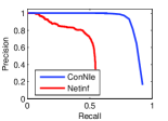
(a) PR Curve (PL)

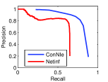
(b) PR Curve (Exp)

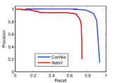
(c) PR Curve (WB)

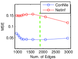
(d) MSE (PL)

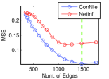
(e) MSE (Exp)

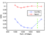
(f) MSE (WB)

Figure 1: (a)-(c): Precision and recall of ConNIe compared to NetInf for the SI diffusion model, run on a synthetical scale-free graph with synthetically generated cascades. Transmission time models used are power law (PL), exponential (Exp), and Weibull (WB). All networks contain 512 nodes, and the weight of each edge was sampled from a uniform random distribution between 0 and 1. For the MLE method, the PR curves were generated by varying the sparsity parameter $\rho$ between 0 and 1000. (d)-(f): Mean square error of the edge transmission probability of the two algorithms. The dotted green line indicates the number of edges in the true network.

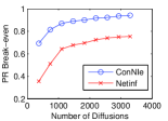
(a) PR Break-even (PL)

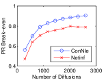
(b) PR Break-even (EXP)

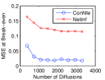
(c) MSE (PL)

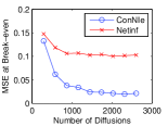
(d) MSE (EXP)

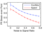
(e) PR vs. Noise/Signal

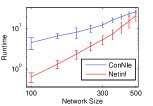
(f) Runtime vs. Network Size

Figure 2: (a)-(b): Precision-Recall break-even point for the two methods as a function of the number of observed cascades, with a power law (PL) and exponential (EXP) transmission distribution. (c)-(d): Mean Square Error at the PR-Break-even point as a function of the number of observed cascades. (e) PR Break-even point versus the perturbation size applied to the infection times.

Figure 1 shows the precision-recall curves for the scale-free synthetic network with the three transmission models $w(t)$. The results for the Erdős-Rényi random graph were omitted due to space restrictions, but they were very similar. Notice our approach achieves the break even point (point where precision equals recall) well above 0.85. This is a notable result: we were especially careful not to generate too many cascades, since more cascades mean more evidence that makes the problem easier. Also in Figure 1 we plot the Mean Squared Error of the estimates of the edge transmission probability $A_{ij}$ as a function of the number of edges in the inferred network. The green vertical line indicates the point where the inferred network contains the same number of edges as the real network. Notice that ConNIe estimates the edge weights with error less than 0.05, which is more than a factor of two smaller than the error of the NetInf algorithm. This, of course, is expected as NetInf assumes the network edge weights are homogeneous, which is not the case.

We also tested the robustness of our algorithm. Figure  2 shows the accuracy (Precision-Recall break-even point as well as edge MSE) as a function of the number of observed diffusions, as well as the effect of noise in the infection times. Noise was added to the cascades by adding independent normally distribution perturbations to each of the observed infection times, and the noise to signal ratio was calculated as the average perturbation over the average infection transmission time. The plot shows that ConNIe is robust against such perturbations, as it can still accurately infer the network with noise to signal ratios as high as 0.4.

3.2 Experiments on Real data

Real social networks. We also experiment with three real-world networks. First, we consider a small collaboration network between 379 scientists doing research on networks. Second, we experiment on a real email social network of 593 nodes and 2824 edges that is based on the email communication in a small European research institute.

For the edges in the collaboration network we simply randomly assigned their edge transmission probabilities. For the email network, the number of emails sent from a person $i$ to a person $j$ indicates the connection strength. Let there be a rumor cascading through a network, and assume the probability that any one email contains this rumor is fixed at $\xi$. Then if person $i$ sent person $j$ $m_{ij}$ emails, the probability of $i$ infecting $j$ with the rumor is $A_{ij}=1-(1-\phi)(1-\xi)^{m_{ij}}$. The parameter $\phi$ simply enforces a minimum edge weight between the pairs who have exchanged least one email. We set $\xi=.001$ and $\phi=.05$.

For the email network we generated cascades using the power-law transmission time model, while for the collaboration network we used the Weibull distribution for sampling transmission times. We then ran the network inference on cascades, and Figure 3 gives the results. Similarly as with synthetic networks our approach achieves break even points of around 0.95 on both datasets. Moreover, the edge transmission probability estimation error is less than 0.03. This is ideal: our method is capable of near perfect recovery of the underlying social network over which a relatively small number of contagions diffused.

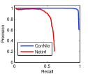
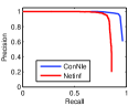
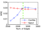
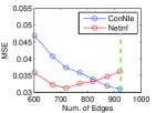
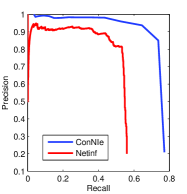
Network estimation	Edge weight error	Recommendation network

Figure 3: The precision-recall curve of the network estimation and the mean-square error (left) of predicted transmission probabilities as a function of number edges being predicted (middle). Top row shows the results for the email network, and the bottom row for the collaboration network. (Right) Precision-recall curve on inferring a real recommendation network based on real product recommendation data.

Real social networks and real cascades. Last, we investigate a large person-to-person recommendation network, consisting of four million people who made sixteen million recommendations on half a million products [14]. People generate cascades as follows: a node (person) $v$ buys product $p$ at time $t$, and then recommends it to nodes $\{w_{1},\dots,w_{n}\}$. These nodes $w_{i}$ can then buy the product (with the option to recommend it to others). We trace cascades of purchases on a small subset of the data. We consider a recommendation network of 275 users and 1522 edges and a set of 5,767 recommendations on 625 different products between a set of these users. Since the edge transmission model is unknown we model it with a power-law distribution with parameter $\alpha=2$.

We present the results in rightmost plot of Figure 3. Our approach is able to recover the underlying social network surprisingly accurately. The break even point of our approach is 0.74 while NetInf scores 0.55. Moreover, we also note that our approach took less than 20 seconds to infer this network. Since there are no ground truth edge transmission probabilities for us to compare against, we can not compute the error of edge weight estimation.

4 Conclusion

We have presented a general solution to the problem of inferring latent social networks from the network diffusion data. We formulated a maximum likelihood problem and by solving an equivalent convex problem, we can guarantee the optimality of the solution. Furthermore, the $l_{1}$ regularization can be used to enforce a sparse solution while still preserving convexity. We evaluated our algorithm on a wide set of synthetic and real-world networks with several different cascade propagation models. We found our method to be more general and robust than the competing approaches. Experiments reveal that our method near-perfectly recovers the underlying network structure as well as the parameters of the edge transmission model. Moreover, our approach scales well as it can infer optimal networks on thousand nodes in a matter of minutes.

One possible venue for future work is to also include learning the parameters of the underlying model of diffusion times $w(t)$. It would be fruitful to apply our approach to other datasets, like the spread of a news story breaking across the blogosphere, a SARS outbreak, or a new marketing campaign on a social networking website, and to extend it to additional models of diffusion. By inferring and modeling the structure of such latent social networks, we can gain insight into positions and roles various nodes play in the diffusion process and assess the range of influence of nodes in the network.

Acknowledgements. This research was supported in part by NSF grants CNS-1010921, IIS-1016909, LLNL grant B590105, the Albert Yu and Mary Bechmann Foundation, IBM, Lightspeed, Microsoft and Yahoo.

References

- [1] A. Ahmed and E. Xing. Recovering time-varying networks of dependencies in social and biological studies. PNAS, 106(29):11878, 2009.
- [2] N. T. J. Bailey. The Mathematical Theory of Infectious Diseases and its Applications. Hafner Press, 2nd edition, 1975.
- [3] A.-L. Barabási and R. Albert. Emergence of scaling in random networks. Science, 1999.
- [4] M. Choudhury, W. A. Mason, J. M. Hofman, and D. J. Watts. Inferring relevant social networks from interpersonal communication. In WWW ’10, pages 301–310, 2010.
- [5] N. Eagle, A. S. Pentland, and D. Lazer. Inferring friendship network structure by using mobile phone data. PNAS, 106(36):15274–15278, 2009.
- [6] J. Friedman, T. Hastie, and R. Tibshirani. Sparse inverse covariance estimation with the graphical lasso. Biostat, 9(3):432–441, 2008.
- [7] L. Getoor, N. Friedman, D. Koller, and B. Taskar. Learning probabilistic models of link structure. JMLR, 3:707, 2003.
- [8] Z. Ghahramani. Learning dynamic Bayesian networks. Adaptive Processing of Sequences and Data Structures, page 168, 1998.
- [9] L. Giot, J. Bader, C. Brouwer, A. Chaudhuri, B. Kuang, Y. Li, Y. Hao, C. Ooi, B. Godwin, et al. A protein interaction map of Drosophila melanogaster. Science, 302(5651):1727, 2003.
- [10] M. Gomez-Rodriguez, J. Leskovec, and A. Krause. Inferring networks of diffusion and influence. In KDD ’10, 2010.
- [11] S. Hill, F. Provost, and C. Volinsky. Network-based marketing: Identifying likely adopters via consumer networks. Statistical Science, 21(2):256–276, 2006.
- [12] R. Jansen, H. Yu, D. Greenbaum, et al. A bayesian networks approach for predicting protein-protein interactions from genomic data. Science, 302(5644):449–453, October 2003.
- [13] G. Kossinets and D. J. Watts. Empirical analysis of an evolving social network. Science, 2006.
- [14] J. Leskovec, L. A. Adamic, and B. A. Huberman. The dynamics of viral marketing. ACM TWEB, 1(1):2, 2007.
- [15] J. Leskovec, L. Backstrom, and J. Kleinberg. Meme-tracking and the dynamics of the news cycle. In KDD ’09, pages 497–506, 2009.
- [16] J. Leskovec and E. Horvitz. Planetary-scale views on a large instant-messaging network. In WWW ’08, 2008.
- [17] J. Leskovec, A. Singh, and J. M. Kleinberg. Patterns of influence in a recommendation network. In PAKDD ’06, pages 380–389, 2006.
- [18] D. Liben-Nowell and J. Kleinberg. The link prediction problem for social networks. In CIKM ’03, pages 556–559, 2003.
- [19] N. Meinshausen and P. Buehlmann. High-dimensional graphs and variable selection with the lasso. The Annals of Statistics, pages 1436–1462, 2006.
- [20] M. Middendorf, E. Ziv, and C. Wiggins. Inferring network mechanisms: the Drosophila melanogaster protein interaction network. PNAS, 102(9):3192, 2005.
- [21] M. Schmidt, A. Niculescu-Mizil, and K. Murphy. Learning graphical model structure using l1-regularization paths. In AAAI, volume 22, page 1278, 2007.
- [22] L. Song, M. Kolar, and E. Xing. Time-varying dynamic bayesian networks. In NIPS ’09.
- [23] B. Taskar, M. F. Wong, P. Abbeel, and D. Koller. Link prediction in relational data. NIPS ’03.
- [24] J. Vert and Y. Yamanishi. Supervised graph inference. NIPS ’05.
- [25] M. J. Wainwright, P. Ravikumar, and J. D. Lafferty. High-dimensional graphical model selection using -regularized logistic regression. In PNAS, 2006.
- [26] J. Wallinga and P. Teunis. Different epidemic curves for severe acute respiratory syndrome reveal similar impacts of control measures. Amer. J. of Epidemiology, 160(6):509–516, 2004.
- [27] S. Wasserman and K. Faust. Social Network Analysis : Methods and Applications. Cambridge University Press, 1994.