The Spatial Clustering of ROSAT All-Sky Survey AGNs
II. Halo Occupation Distribution Modeling of the Cross Correlation Function

Abstract

This is the second paper of a series that reports on our investigation of the clustering properties of AGNs in the ROSAT All-Sky Survey (RASS) through cross-correlation functions (CCFs) with Sloan Digital Sky Survey (SDSS) galaxies. In this paper, we apply the Halo Occupation Distribution (HOD) model to the CCFs between the RASS Broad-line AGNs with SDSS Luminous Red Galaxies (LRGs) in the redshift range $0.16<z<0.36$ that was calculated in paper I. In our HOD modeling approach, we use the known HOD of LRGs and constrain the HOD of the AGNs by a model fit to the CCF. For the first time, we are able to go beyond quoting merely a ‘typical’ AGN host halo mass, $M_{\rm h}$, and model the full distribution function of AGN host dark matter halos. In addition, we are able to determine the large-scale bias and the mean $M_{\rm h}$ more accurately. We explore the behavior of three simple HOD models. Our first model (Model A) is a truncated power-law HOD model in which all AGNs are satellites. With this model, we find an upper limit to the slope ($\alpha$) of the AGN HOD that is far below unity. The other two models have a central component, which has a step function form, where the HOD is constant above a minimum mass, without (Model B) or with (Model C) an upper mass cutoff, in addition to the truncated power-law satellite component, similar to the HOD that is found for galaxies. In these two models we find that the upper limits on $\alpha$ are still below unity, with $\alpha\lesssim 0.95$ and $\alpha\lesssim 0.84$ for Model B and C respectively. Our analysis suggests that the satellite AGN occupation increases slower than, or may even decrease with, $M_{\rm h}$ in contrast to the satellite HODs of luminosity-threshold samples of galaxies, which, in contrast, grow approximately as $\langle N_{\rm s}\rangle\propto M_{\rm h}^{\alpha}$ with $\alpha\approx 1$. These results are consistent with observations that the AGN fraction in groups and clusters decreases with richness.

1. Introduction

Investigating how active galactic nuclei (AGNs) are distributed in the Universe provides a clue as to the physical conditions in which accretion onto supermassive black holes (SMBH) takes place. After the formation of galaxies in the universe, at any given time in the history of the Universe, only a small fraction of galaxies show AGN activity. It is known that almost all galaxies with a spheroidal component contain a SMBH, and that the BH mass is closely related to the mass or the velocity dispersion of the spheroidal component (e.g., Ferrarese & Merritt 2000; Gebhardt et al. 2000; Marconi & Hunt 2003; Häring & Rix 2004; Shankar 2009 for review). This means that most galaxies have likely had one or more brief AGN periods, during which the central SMBH grows in such a way that the growth of the SMBH and the formation of the spheroidal component are tightly related. The question of when and under what physical conditions the accretion takes place is important in understanding not only the origin and evolution of SMBHs but also the origin and evolution of galaxies. Many models postulate that AGN activity is merger-driven, especially those with high luminosities (i.e., QSOs), (e.g., Wyithe & Loeb 2002; Hopkins et al. 2006). On the other hand, for lower-luminosity AGNs, processes internal to the galaxy such as galaxy disk instabilities, may be important (Kauffmann et al. 2007; Hasinger 2008). Different mechanisms may be responsible for triggering AGN activity at different redshifts or luminosities.

Large-scale clustering properties of AGNs provide important clues as to the physical process(es) that are responsible for the SMBH accretion. The large-scale clustering amplitude reflects, through the bias parameter $b$, the typical mass of the dark matter halos (DMH) in which AGN reside (Sheth & Tormen 1999; Sheth et al. 2001; Tinker et al. 2005). Thus exploring the clustering properties of AGNs at different redshifts, luminosities, and AGN types to probe the masses of the DMHs that host them, provides us with important clues in understanding constraints on SMBH growth in a cosmological context.

Clustering measurements of X-ray point sources have been made whenever new large-scale surveys have been completed, through angular correlation functions (e.g. Puccetti et al. 2006; Miyaji et al. 2007; Ueda et al. 2008; Plionis et al. 2008; Ebrero et al. 2009b). When redshifts for a complete sample become available, three-dimensional (3D) correlation functions can then be computed (e.g., Mullis et al. 2004; Yang et al. 2006; Gilli et al. 2009; Cappelluti et al. 2010). Redshift information provides a huge leap in clustering measurements both in terms of the statistical accuracy as well as in removing systematic errors associated with model assumptions in making Limber’s de-projection (Limber 1954). However, even with redshift information, small number statistics has limited the accuracy of correlation function (CF) measurements, especially through the auto-correlation function (ACF) of the AGNs themselves. The situation can be improved by measuring the cross-correlation function (CCF) of AGNs with a galaxy sample that has a much higher space density. In order to facilitate a CCF analysis, one needs an extensive galaxy redshift surveys with common sky and redshift coverage as the AGN redshift surveys. With recent large-scale survey projects, measurements of AGN clustering through CCF with galaxies are now emerging (e.g., Li et al. 2006; Coil et al. 2007, 2009; Hickox et al. 2009; Padmanabhan et al. 2009; Mountrichas et al. 2009).

While the ROSAT All Sky Survey (RASS) (Voges et al. 1999), most of which was conducted during the first half year of the ROSAT mission (mostly in 1990), produced a catalog of $\approx 120,000$ X-ray point sources, the availability of a comprehensive redshift survey of RASS-selected AGNs was limited until a RASS-Sloan Digital Sky Survey (SDSS) matched AGN catalog became available (Anderson et al. 2003, 2007). In view of this, we initiated a series of studies of the clustering properties of low redshift AGNs in the RASS-SDSS sample through the CCF analysis with SDSS galaxies. In Krumpe et al. (2010, hereafter paper I), we reported our results on our CCF analysis between broad-line AGNs in RASS that have been identified with SDSS (Anderson et al. 2007) and the SDSS Luminous Red Galaxies (LRGs) (Eisenstein et al. 2001) in the redshift range $0.16<z<0.36$.

Through these efforts to measure the AGN ACF/CCF, the masses of the DMHs where AGN activity occurs are being gradually uncovered. Most results measuring the 3D correlation functions of X-ray selected AGNs indicate that the typical DMH mass in which these AGN reside is in the range $12\lesssim\log M_{\rm h}[h^{-1}M_{\rm sun}]\lesssim 13.5$ at both low ($z\lesssim 0.4$) and high ($z\approx 1$) redshifts (e.g., paper I; Coil et al. 2009; Gilli et al. 2009; Cappelluti et al. 2010). Optically-selected QSOs, typically representing a high redshift, high luminosity AGN population, are associated with DMHs with a typical mass in the range $12\lesssim\log M_{\rm h}[h^{-1}M_{\rm sun}]\lesssim 13$ (e.g. Porciani et al. 2004; Coil et al. 2007; Shen et al. 2007; Ross et al. 2009). It appears that the luminosity dependence of AGN clustering may be different at different redshifts. In paper I, we show that among broad-line AGN, high X-ray luminosity AGNs are more strongly clustered than lower X-ray luminosity AGN at z$\approx 0.3$. At $z\approx 1$, however, low luminosity X-ray selected AGNs are more strongly clustered than optical QSOs (Coil et al. 2009). This apparent difference may be caused by a non-monotonic luminosity dependence and/or AGN type dependence of biasing rather than a dependence on redshift. What is needed is to explore AGN clustering across wider ranges in luminosity-redshift space to break this degeneracy.

In interpreting the correlation function measurements, most previous studies use the large scale bias ($b$) of AGNs to infer the associated typical DMH mass using linear growth and linear biasing schemes. Strictly speaking, this is only valid for the correlation function measurements on sufficiently large scales ($r\gtrsim 1-2h^{-1}$ Mpc). Non-linear modeling through the Halo Occupation Distribution (HOD) framework (e.g. Peacock & Smith 2000; Seljak 2000; Cooray & Sheth 2002) is imperative to accurately interpret and make full use of the correlation function measurements. In this framework, the mean number of the sample objects in the DMH ($\langle N\rangle$) is modeled as a function of the DMH mass ($M_{\rm h}$). Then the two-point correlation function is modeled as the sum of the contributions of pairs from the same DMH (1-halo term) and those from different DMHs (2-halo term). This method has been used extensively to interpret galaxy correlation functions (e.g. Hamana et al. 2004; Tinker et al. 2005; Phleps et al. 2006; Zheng et al. 2007; Zehavi et al. 2010; Zheng et al. 2009, hereafter Z09) to constrain how various galaxy samples are distributed among DMHs as well as whether these galaxies occupy the centers of the DMHs or are satellite galaxies (Kravtsov et al. 2004; Zheng et al. 2005).

Partially due to the low number density of AGNs, there have been few results in the literature interpreting AGN correlation functions using HOD modeling, where the small-scale clustering measurements are essential. Padmanabhan et al. (2009) discussed qualitative HOD constraints on their LRG-optical QSO CCF, where they argued that the acceptable models include those in which $>25$% of their QSOs are satellites and those in which QSOs are a random subsampling of a luminosity-threshold sample of galaxies. Shen et al. (2010) also used the HOD modeling approach to binary pairs of QSOs at $3\lesssim z\lesssim 4$ and conclude that they favor a model in which $\gtrsim 10$% of the QSOs are satellites.

In this paper, we apply the HOD model to the CCFs of the RASS broad-line AGNs (hereafter, simply referred to as AGNs) and SDSS LRGs obtained in paper I. The HOD modeling has allowed us to model the CCFs beyond simple power-law fits and to investigate constraints on how these AGNs are distributed among DMHs as a function of halo mass. While almost all previous HOD modeling studies apply the method to ACFs, here we apply the HOD modeling approach to the CCF. With this method, we use the previously estimated LRG HOD to model the AGN HOD by fitting to the measured AGN-LRG CCF. In our analysis, we take advantage of the LRG HOD of Z09, which is based on the well-measured LRG ACF from SDSS (Zehavi et al. 2005b). This approach was taken by Z09 in modeling LRG-$L_{*}$ galaxy CCFs, assuming that the LRGs are central galaxies of the DMHs and that the $L_{*}$ galaxies are satellite galaxies upon the calculation of the 1-halo term.

In this paper, we present a comprehensive explanation of the HOD analysis that can be applied to general cases, and then we apply the method to our AGN-LRG CCF.

The scope of the paper is as follows. In sect. 2, we summarize the samples used in paper I and the basic methods of CCF calculations. In Sect. 3, we explain our basic modeling procedure of the LRG ACF, which is used as a template to apply the HOD modeling to the AGN-LRG CCF. In Sect. 4, we show our results on the AGN HODs. Sect. 5 discusses our results, including a comparison with the results from paper I and the astrophysical implications of our constraints on the AGN HOD obtained here. Finally, Sect. 6 summarizes important consequences from our analysis and concludes our discussion.

Throughout the paper, all distances are measured in comoving coordinates and given in units of $h^{-1}$ Mpc, where $h=H_{\rm 0}/100$ km s^-1. We also use the symbol $h_{70}=H_{\rm 0}/70$ km s^-1 for X-ray luminosities, while $h=1$ is used to express optical absolute magnitudes, for consistency with referenced articles. We use a cosmology with $h=0.7$, $\Omega_{\rm M}=0.3$, $\Omega_{\rm\Lambda}=0.7$, $\sigma_{8}=0.8$, $\Omega_{\rm baryon}=0.047$ and $n_{\rm s}=1$, which are consistent with the most updated WMAP cosmology as of writing this paper (Spergel et al. 2003). The symbol $\log$ signifies a base-10 logarithm, while a natural logarithm is expressed by an $\ln$.

2. The RASS AGN-LRG CCF Measurements

In paper I, we calculate the CCFs between AGNs and the LRG, as well as the LRG ACF in the redshift range $0.16<z<0.36$. Basic properties of the sample used in that paper are repeated here in Table 1. The rationale and strategies of the sample selection are discussed in paper I in detail, including a redshift-$L_{\rm x}$ diagram of the AGN sample (Fig. 1 of paper I). Here we briefly summarize the sample selection and CF calculations below.

We use the AGN sample from the RASS-SDSS matched AGN catalog by Anderson et al. (2003, 2007), which is based on the SDSS Data Release (DR) 5. In order to make a well-defined, uniform AGN sample, we only include broad lines AGNs. For the reference sample, we extract LRGs from the SDSS Catalog Archive Server Jobs System using the flag “galaxy_red”, which is based on the selection criteria defined in (Eisenstein et al. 2001). We create a volume-limited spectroscopic LRG sample with $-23.2<M_{g}^{z=0.3}<-21.2$ and $0.16<z<0.36$. The AGN sample is also limited to this redshift range. In order to obtain the largest common geometry between the AGNs and LRGs with public geometry and completeness files (Blanton et al. 2005), we limit our sample to the SDSS DR4+ geometry . The selected geometry covers an area of 5468 deg². The AGN sample is further divided into high $L_{\rm X}$ and low $L_{\rm X}$ samples. The numbers of LRGs and AGNs used in our CCF measurements are listed in Table 1.

Table 1Properties of the LRG and RASS-AGN samples

sample	$z$	$M_{g}^{z=0.3}$ range		$<n_{\rm LRG}>$		$<M_{g}^{z=0.3}>$
name	range	[mag]	number	[$h^{3}$ Mpc-3]	$<z>$	[mag]
LRG sample	$0.16<z<0.36$	$-23.2<M_{g}^{z=0.3}<-21.2$	45899	$9.6\times 10^{-5}$	0.28	-21.71
		$\log L_{\rm X}$ range		$<n_{\rm AGN}>$		$\log<L_{\rm X}>$
	$z$-range	range [$h_{70}^{-2}$erg s-1]	number	[$h^{3}$ Mpc-3]	$<z>$	[$h_{70}^{-2}$ erg s-1]
All RASS-AGN sample	$0.16<z<0.36$	$43.7\lesssim\log L_{\rm X}\lesssim 44.7$	1552	$6.0\times 10^{-5}$	0.25	44.17 (44.16)
High $L_{\rm X}$ RASS-AGN sample	$0.16<z<0.36$	$44.3<\log L_{\rm X}\lesssim 44.9$	562	$1.2\times 10^{-6}$	0.28	44.58 (44.53)
Low $L_{\rm X}$ RASS-AGN sample	$0.16<z<0.36$	$43.6\lesssim\log L_{\rm X}\leq 44.3$	990	$5.8\times 10^{-5}$	0.24	43.95 (44.16)

In calculating the AGN-LRG CCFs and the LRG ACF, we use the classic Davis & Peebles (1983) estimator, in a two-dimensional (2D) grid in the $(r_{\rm p},\pi)$ space, where $r_{\rm p}$ is the projected distance and $\pi$ is the line-of-sight separation (both in comoving coordinates):

$$\xi(r_{\rm p},\pi)=\frac{D_{1}D_{2}(r_{\rm p},\pi)}{D_{1}R_{2}(r_{\rm p},\pi)}-1,$$ (1)

in which the subscripts 1 and 2 identify the sample, $D_{1}D_{2}$ is the number of pairs between real samples, and $D_{1}R_{2}(r_{\rm p},\pi)$ is the number of pairs between real sample 1 and random sample 2. For the AGN-LRG CCF, the sample 1 is the AGN sample and the sample 2 is the LRG sample, while for the LRG ACF, both sample 1 and sample 2 are the same LRG sample. We use Eq. 1 rather than that proposed by Landy & Szalay (1993) because Eq. 1 requires a random sample for only sample 2 (in our case, LRGs). This is important due of the difficulty in generating a random sample for a RASS-based AGN catalog. ROSAT is sensitive to soft X-rays, which are subject to absorption by neutral hydrogen. The variation in the column density across the sky due to neutral gas in our galaxy, combined with the diversity of the X-ray spectra of AGN, makes it very difficult to model the spatial variation in the detection limit of the AGNs, which is essential in generating a random sample.

We then calculate the projected correlation function:

$$w_{\rm p}(r_{\rm p})=2\int_{0}^{\pi_{\rm max}}\xi(r_{\rm p},\pi)d\pi,$$ (2)

where the upper bound of the integral ($\pi_{\rm max}$) is determined by the saturation of the integral. We take $\pi_{\rm max}=80$ and $40h^{-1}$ Mpc for the LRG ACF and AGN-LRG CCF respectively. The reasoning for these choices is explained in paper I.

In paper I, we further calculate the inferred AGN ACF, $w_{p}(AGN|AGN)$, from the AGN-LRG CCF $w_{p}(AGN|LRG)$ and LRG ACF $w_{p}(LRG|LRG)$, assuming a linear biasing scheme:

$$w_{p}(AGN|AGN)=\frac{\left[w_{p}(AGN|LRG)\right]^{2}}{w_{p}(LRG|LRG)}.$$ (3)

We then fit $w_{p}(AGN|AGN)$ with a power-law form and derive the AGN bias parameters and typical masses of the DMH in which the AGNs reside, based on the power-law fits.

In this paper, instead of using the inferred AGN ACF as in Paper I, we directly model the CCF, $w_{p}(AGN|LRG)$, with an HOD analysis, as $w_{p}(AGN|LRG)$ has been directly derived from the observations and does not depend on a linear biasing approximation. The comparison of results from paper I and this paper are discussed below in Sect. 5.1.

3. Modeling the Halo Occupation Distribution

3.1. Model Ingredients

In performing the HOD modeling, we consider that galaxies and AGNs are associated with DMHs, the mass function of which (per comoving volume per $dM_{\rm h}$) is denoted by $\phi(M_{\rm h})\,dM_{\rm h}$, where $M_{\rm h}$ is the dark matter halo mass. We use $\phi(M_{\rm h})$ based on Sheth & Tormen (1999), which is in good agreement with later analyses by Sheth et al. (2001) and Jenkins et al. (2001). A DMH may contain one or more galaxies and/or AGNs that are included in our samples. We then model the two-point projected correlation function as the sum of two terms,

$$w_{\rm p}(r_{\rm p})=w_{\rm p,1h}(r_{\rm p})+w_{\rm p,2h}(r_{\rm p}),$$ (4)

where the terms are:

• the 1-halo term (denoted by a subscript “1h”), where both of the objects occupy the same DMH, and

• the 2-halo term (denoted by a subscript “2h”), where each of the pair of objects occupies a different DMH.

Recent articles prefer to define $\xi_{\rm 1h}$ such that the total 3D correlation function is expressed by $\xi=(1+\xi_{\rm 1h})+\xi_{\rm 2h}$ (Tinker et al. 2005; Zheng et al. 2005; Blake et al. 2008), instead of $\xi=\xi_{\rm 1h}+\xi_{\rm 2h}$, as used in older articles. This is because $1+\xi$ represents a quantity that is proportional to the number of pairs, and allows one to express each of the 1- and 2-halo terms consistently. In this case, the number of pairs is $\propto 1+\xi=[1+\xi_{\rm 1h}]+[1+\xi_{\rm 2h}]$. In this new convention, our $w_{\rm p,1h}$ represents the projection of $1+\xi_{\rm 1h}$ rather than $\xi_{\rm 1h}$, i.e.,

$$w_{\rm p,1h}(r_{\rm p})=\int_{-\infty}^{\infty}\left[1+\xi_{\rm 1h}\left(r_{\rm p},\pi\right)\right]d\pi.$$ (5)

Similarly, we express the power spectrum of the distribution of the objects in terms of the 1- and 2-halo term contributions:

$$P(k)=P_{\rm 1h}(k)+P_{\rm 2h}(k),$$ (6)

with

$$w_{\rm p,1h}(r_{\rm p}) = \int\frac{k}{2\pi}P_{\rm 1h}(k)J_{0}(kr_{\rm p})dk$$

$$w_{\rm p,2h}(r_{\rm p}) = \int\frac{k}{2\pi}P_{\rm 2h}(k)J_{0}(kr_{\rm p})dk,$$ (7)

where $J_{0}(x)$ is the zeroth-order Bessel function of the first kind.

In the case of modeling the ACF of a sample, the 2-halo term of the power spectrum can be approximated by (Cooray & Sheth 2002)

$$P_{\rm 2h}(k)\approx b^{2}P_{\rm lin}(k,z),$$ (8)

where $b$ is the bias parameter of the sample, which we model as

$$b=\frac{\int b_{\rm h}(M_{\rm h})\langle N\rangle(M_{\rm h})\phi(M_{\rm h})dM_{\rm h}}{\int\langle N\rangle(M_{\rm h})\phi(M_{\rm h})dM_{\rm h}}.$$ (9)

For the linear power spectrum, $P_{\rm lin}(k,z)$, we use the primordial power spectrum with $n_{\rm s}=1$ and a transfer function calculated using the fitting formula of Eisenstein & Hu (1998) under our assumed cosmology (Sect. 1). For the mass-dependent bias parameter of DMHs, $b_{\rm h}(M_{\rm h})$, we use Eq. (8) of Sheth et al. (2001) with recalibrated parameter values by Tinker et al. (2005) (see their Appendix A).

In calculating the 1-halo term, the usual assumption is that the radial distribution of the involved objects that are not at the center of the halo – objects that are satellites – follows the mass profile of the DMH itself, i.e., there is no internal biasing. Following Zheng et al. (2009), whose results will be used later in this work, we use the Navarro et al. (1997) (NFW) profile for the DMH density distribution, which is still a popular choice for representing DMH profiles, although other parametrizations exist in the literature (e.g. Knollmann et al. 2008; Stadel et al. 2009). We express the Fourier transform of the NFW profile of the DMH with mass $M_{\rm h}$, normalized such that volume integral up to the virial radius is unity, by $y(k,M_{\rm h})$. Again, in the case of the ACF,

$$P_{\rm 1h}(k) = \frac{1}{(2\pi)^{3}n^{2}}\int\phi(M_{\rm h})[\langle N_{\rm c}N_{\rm s}\rangle(M_{\rm h})y(k,M_{\rm h})+$$ (10)

$$\langle N_{\rm s}(N_{\rm s}-1)\rangle(M_{\rm h})|y(k,M_{\rm h})|^{2}]dM_{\rm h},$$

where $N_{\rm c}$ and $N_{\rm s}$ are the numbers of the objects in the sample per DMH as a function of $M_{\rm h}$ for those that are at the center of the halos (central) and those that are off center (satellites) respectively, while $n=\int\langle N\rangle(M_{\rm h})\phi(M_{\rm h})dM_{\rm h}$ is their overall space density (Hamana et al. 2004; Seljak 2000).

The HOD model is calculated using a set of software we have developed, based partially on a code developed by J. Peacock for the use in Peacock & Smith (2000) and Phleps et al. (2006). Our software includes a number of improvements over their code, most notably by including the application of the HOD modeling to a CCF. We note, however, that in our analysis we do not include some recent improvements in modeling the 2-halo term (Zheng et al. 2005; Tinker et al. 2005; Zheng et al. 2009). The neglected factors include the convolution of the DMH profile to the 2-halo term and the scale-dependent bias. In addition, if a pair of objects are closer than the sum of the virial radii of their parent halos, the pair should not be counted in the 2-halo term; this effect is neglected. These improvements have enabled those authors to make accurate modelings of, e.g., the ACF of SDSS galaxies, where the correlation functions can be measured to a few percent level at $r_{\rm p}\approx 1h^{-1}$ Mpc. However, as AGNs have a much smaller number density, the errors on our CCF measurements are $\gtrsim 20$% (paper I) at this $r_{\rm p}$, where these improvements are important. Therefore the effects of these recent improvements by other authors are estimated to be within the 1$\sigma$ measurement errors of the CCF.

3.2. The HOD modeling of the AGN-LRG CCF

In this subsection, we explain the application of the HOD modeling to the CCF between AGNs and LRGs (or more generally, between any two different populations). Using the HOD of the LRGs as a template, which has been accurately constrained by Z09 using the LRG ACF measured by Zehavi et al. (2005b), we constrain the HOD of the AGNs by fitting to the AGN-LRG CCF. A similar approach has been made by Z09 to model the CCF between LRGs and $L_{*}$ galaxies, where they assumed that the LRGs are at the halo centers and the $L_{*}$ galaxies are satellites in the 1-halo term calculation. Since LRGs occupy the centers of almost all massive DMHs ($\log M_{\rm h}\gtrsim 14\,[h^{-1}M_{\sun}]$, Z09), this is a good approximation for their LRG-$L_{*}$ galaxy CCF as well as for our AGN-LRG CCF. However, for completeness, we develop a formulation of the HOD modeling that includes more general cases. Hereafter, the quantities for AGNs are represented by a subscript “A”, LRGs by “G” (representing galaxies), and CCF between the two by “AG”. We denote the LRG HODs at the halo center and of satellites by $\langle N_{\rm G,c}\rangle(M_{\rm h})$ and $\langle N_{\rm G,s}\rangle(M_{\rm h})$, respectively. Now $\langle N_{\rm G}\rangle(M_{\rm h})=\langle N_{\rm G,c}\rangle(M_{\rm h})+\langle N_{\rm G,s}\rangle(M_{\rm h})$. Likewise, the HODs of the AGNs at the halo centers, of satellites, and the sum of the two are denoted by $\langle N_{\rm A,c}\rangle(M_{\rm h})$, $\langle N_{\rm A,s}\rangle(M_{\rm h})$ and $\langle N_{\rm A}\rangle(M_{\rm h})$.

In our approximate treatment, the two halo term can be expressed as follows. Let the linear bias parameters of the LRGs and AGNs be $b_{\rm G}$ and $b_{\rm A}$ respectively:

$$b_{\rm G} = \frac{\int b_{\rm h}(M_{\rm h})\langle N_{\rm G}\rangle(M_{\rm h})\phi(M_{\rm h})dM_{\rm h}}{\int\langle N_{\rm G}\rangle(M_{\rm h})\phi(M_{\rm h})dM_{\rm h}}$$ (11)

$$b_{\rm A} = \frac{\int b_{\rm h}(M_{\rm h})\langle N_{\rm A}\rangle(M_{\rm h})\phi(M_{\rm h})dM_{\rm h}}{\int\langle N_{\rm A}\rangle(M_{\rm h})\phi(M_{\rm h})dM_{\rm h}}.$$ (12)

Then the two halo term of the power spectrum corresponding to the CCF (cross power spectrum) can be expressed by

$$P_{\rm AG,2h}(k)\approx b_{\rm A}b_{\rm G}P_{\rm lin}(k).$$ (13)

The 1-halo term is composed of three terms:

$$P_{\rm AG,1h}(k) = \frac{1}{(2\pi)^{3}n_{\rm A}n_{\rm G}}\int\phi(M_{\rm h})\times$$ (14)

$$[\langle N_{\rm A,c}N_{\rm G,s}+N_{\rm A,s}N_{\rm G,c}\rangle(M_{\rm h})\,\,y(k,M_{\rm h})+$$

$$\langle N_{\rm A,s}N_{\rm G,s}\rangle(M_{\rm h})\,\,|y(k,M_{\rm h})|^{2}]\,dM_{\rm h},$$

provided that no object is in common between the AGN and LRG samples (which is the case in our CCF). In this case, the relation

$$\langle N_{\rm A,x}N_{\rm G,y}\rangle(M_{\rm h})=\langle N_{\rm A,x}\rangle(M_{\rm h})\langle N_{\rm G,y}\rangle(M_{\rm h})$$ (15)

holds, where the subscripts x and y represent any combination of the subscripts s and c, except for the case both are c’s. This relation is exact even if $\langle N\rangle\lesssim 1$, where one has to use the exact Poisson distribution for the probability distribution of having exactly $N$ objects in a halo (sometimes called a sub-Poissonian case). The relation $\langle N_{\rm A,c}N_{\rm G,s}+N_{\rm A,s}N_{\rm G,c}\rangle=\langle N_{\rm A,c}N_{\rm G,s}\rangle+\langle N_{\rm A,s}N_{\rm G,c}\rangle$ also holds.

Even in cases where there are objects in common between the two samples, the above discussion does not change for the central-satellite pairs, because the two objects are surely different. However, the existence of the common objects makes assumptions behind the third term in the integrand of Eq. 14 invalid. A detailed discussion of this case is beyond the scope of the present paper, and will be made in a future paper.

3.2.1 The LRG HOD

The HOD of the LRGs has been extensively studied by Z09 based on the ACF measurements of the LRGs by Zehavi et al. (2005b) using SDSS Data Release (DR) 3. Their $\langle N_{\rm G,s}\rangle(M_{\rm h})$ model has essentially five parameters, which are the values at five $M_{\rm h}$ points, and they have spline-interpolation values between these points. They take an elaborate parametrization of $\langle N_{\rm G,c}\rangle(M_{\rm h})$, which is an integration of a luminosity-dependent smoothed step-function, where the value increases from 0 (at low $M_{\rm h}$) to 1 (at high $M_{\rm h}$), with a transition following a luminosity-dependent error function.

In paper I, we re-calculate the LRG ACF for the $0.16<z<0.36$, $-23.2<M_{g}<-21.2$ sample based on DR4+, using $\approx$46,000 LRGs, instead of $\approx$30,000 LRGs from DR3 used by Zehavi et al. (2005b). We obtain practically the identical ACF to that calculated by Zehavi et al. (2005b). Since we want to use exactly the same model and the same LRG sample between the LRG ACF and the LRG-AGN CCF, we derive the best-fit LRG HOD to our DR4+ sample using our software. However, instead of newly exploring the full parameter space, we take advantage of the analysis in Z09 to find the HODs that give the best fit to our data by tweaking their LRG HODs as follows. Fig. 1 (b) of Z09 shows the $\Delta\chi^{2}=4$ upper and lower bounds of the HODs separately for the central and satellite LRGs. For the satellites, we start with their $\Delta\chi^{2}=4$ upper and lower bounds, denoted by $N_{\rm Z,s}^{\rm u}$ and $N_{\rm Z,s}^{\rm l}$ respectively. We then interpolate between these curves:

$$\langle N_{\rm G,s}\rangle(M_{\rm h})=(1-f)\langle N_{\rm Z,s}^{\rm l}\rangle(M_{\rm h})+f\langle N_{\rm Z,s}^{\rm u}\rangle(M_{\rm h}),\\$$

where $f$ is a weight parameter in the linear interpolating procedure.

For the central LRGs, we shift their central HOD ($N_{\rm Z,c}$) horizontally by $d$ in $\log M_{\rm h}$:

$$\langle N_{\rm G,c}\rangle(M_{\rm h})=\langle N_{\rm Z,c}\rangle(M_{\rm h}10^{d})\\$$

We tweak $N_{\rm G,c}$ horizontally because of the $\langle N_{\rm G,c}\rangle(M_{\rm h})\leq 1$ constraint. In calculating $\langle N_{\rm s}(N_{\rm s}-1)\rangle(M_{\rm h})$ of the LRG ACF based on the above HODs, we calculate the mean value using the exact Poisson statistics in the small number case ($\langle N_{\rm s}\rangle\leq 10.0$), while we use $\langle N_{\rm s}\rangle(\langle N_{\rm s}\rangle-1)$ for larger values. As a whole, our model has two “tweak” parameters, $f$ and $d$.

We calculate a series of model ACFs at $z=0.28$ (the average redshift of our sample, see Table 1) in a parameter space grid exhaustively over a rectangular area in the $(f,d)$ space that is large enough to include all the region with $\Delta\chi^{2}\lesssim 5$. The grid spacings are 0.03 and 0.003 for $f$ and $d$ respectively.

Then we fit the model to the data by minimizing $\chi^{2}$, taking the correlation of errors and the total number density of LRGs ($n_{\rm LRG}$) into account:

$$\chi^{2} = \sum_{ij}\{[w_{\rm p}(r_{{\rm p},i})-w_{\rm p}^{\rm mdl}(r_{{\rm p},i})]M^{-1}_{ij}\times$$ (16)

$$[w_{\rm p}(r_{{\rm p},j})-w_{\rm p}^{\rm mdl}(r_{{\rm p},j})]\}+$$

$$(n_{\rm LRG}-n_{\rm LRG}^{\rm mdl})^{2}/\sigma_{n_{\rm LRG}}^{2},$$

where the quantities from the model are indicated by a superscript “mdl”, $M$ is the covariance matrix, and $\sigma_{n_{\rm LRG}}$ is the 1$\sigma$ error of the LRG number density. The covariance matrix and $\sigma_{n_{\rm LRG}}$ are estimated using the jackknife resampling method (see paper I). During the minimization process, the models $w_{\rm p}^{\rm mdl}(r_{{\rm p},i})$ are calculated by interpolating from the four nearest grid points in the parameter space computed above. The minimization is performed using the MINUIT package distributed as a part of the CERN program library. Including the number density term in $\chi^{2}$ gives important parameter constraints, not only on the overall normalization, but also the shape. This is because $N_{\rm G,c}$, by definition, has the absolute maximum value of unity (as there can not be more than one central galaxy in a halo), and for the LRGs, the value saturates at 1 for $M_{\rm h}\gtrsim 10^{\rm 14}h^{-1}\,M_{\odot}$. With this constraint, $n_{\rm LRG}$ becomes sensitive to the combination of the relative normalizations between $N_{\rm G,c}$ and $N_{\rm G,s}$ and the “cut-off” mass of $N_{\rm G,c}$. For the LRG sample defined in paper I, $n_{\rm LRG}=(9.56\pm 0.13)\times 10^{-5}h^{-3}$ Mpc^-3. In performing the fits, we use only the data points that are dominated by either the 1-halo or 2-halo terms, excluding the transition region ($0.46<r_{\rm p}[h^{-1}{\rm Mpc}]<2.8$). In this transition region, our model ACF becomes inaccurate due to our approximations, especially in neglecting the halo-exclusion effect in the 2-halo term, as described above in Sect 3.1. We use the data points down to $r_{\rm p}=0.2\,[h^{-1}{\rm Mpc}]$, which is slightly below the lower $r_{\rm p}$ limit used in paper I. Our measurements to this scale are consistent with those measure by Masjedi et al. (2006).

Our best fit model has ‘tweak’ parameter values of $f=1.21(1.12;1.29)$ and $d=-0.087(-0.095;-0.083)$, where the 68% confidence ranges for two interesting parameters ($\Delta\chi^{2}<2.3$) are given in parentheses. Our HODs are slightly higher than those measured by Z09, probably because we include a data point at $r_{\rm p}=0.2\,[h^{-1}{\rm Mpc}]$ and we use a slightly different linear power spectrum. The best-fit model $w_{\rm p}(r_{\rm p})$ is compared with the observation as well as the Z09 model in Fig. 1(a). The corresponding HODs ($\langle N_{\rm G,s}(M_{\rm h})\rangle$, $\langle N_{\rm G,c}(M_{\rm h})\rangle$ and the total) are shown in Fig. 1(b), and confidence contours in the ($d$,$f$) space are shown in Fig. 1(c).

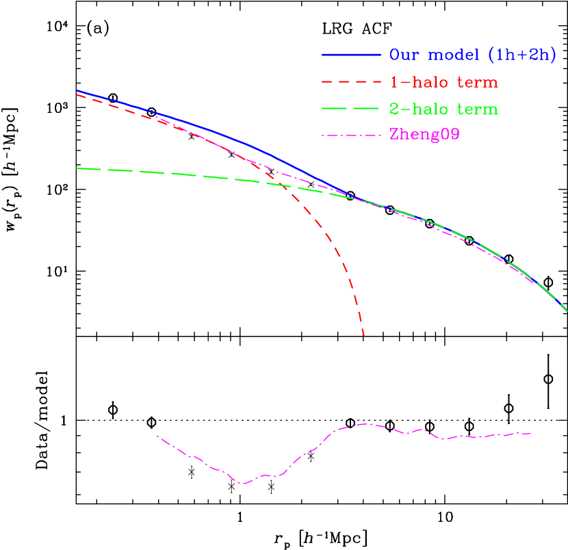
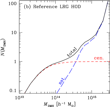
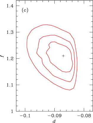
Figure 1.— (a) The ACF of the luminous red galaxy (LRG) sample and the best-fit HOD model (upper panel) with residuals (lower panel). The data points and error bars show our measurements of the LRG ACF. The circles show the data points used for the fit, while the crosses show those excluded. The dashed (green), long-dashed (green) and thick-dashed lines show the 1-halo term, 2-halo term, and the total respectively. The dot-dashed (magenta) curve represents the best-fit model by Z09. Our simplified model fits well in the regimes where the 1-halo term and 2-halo terms dominate. (b) Our best fit HODs for the central LRGs (red dashed line), satellite LRGs (blue long-dashed line), and the total. (c) Confidence contours in the $d$-$f$ space (see text for details). The confidence levels are $\Delta\chi^{2}=1.0,2.3$ and 4.6. The cross shows the best-fit values.

3.2.2 The AGN HOD

With the LRG HOD in hand, we come to our main purpose of obtaining constraints on the HOD of the AGNs in the RASS-SDSS survey.

As a parametrized form of the AGN HOD, we first try a simple truncated power-law form, assuming that all the AGNs are satellites (Model A):

$$\langle N_{\rm A,s}\rangle\propto M_{\rm h}^{\alpha}\Theta(M_{\rm h}-M_{\rm cr}),\,\,\langle N_{\rm A,c}\rangle=0$$ (17)

where $\Theta(x)$ is the step function ($=1$ at $x\geq 0$; $=0$ at $x<0$), $M_{\rm cr}$ is a critical DMH mass below which the HOD is zero, and $\alpha$ is a power-law slope of the HOD above $M_{\rm cr}$. While formally we are assuming that all AGNs are satellites, the HOD constraints obtained from this assumption can be applied fairly to the sum of the central and satellite AGNs in cases where the AGN activity in the central galaxy of high mass $\log\,M_{\rm h}[h^{-1}M_{\sun}]\gtrsim 13.5$ DMHs is suppressed. For simplicity of explanation, we visualize the HOD of the central LRG as a step function with a step at $\log\,M_{\rm h}[h^{-1}M_{\sun}]=13.5$, and refer the DMH mass roughly above (below) this cut as higher (lower) mass. There is no contribution to the 1-halo term at lower mass DMHs, since the 1-halo term requires both AGNs and LRGs to reside at the same DMH mass. Since there is in practice no distinction between central and satellite AGNs in the 2-halo term (Eq. 13), whether the AGNs in low mass DMHs are satellites or central makes no difference to the CCF, and indeed this model can fairly accommodate a case where a low-mass halo represents one galaxy (halo) at the center. At higher masses, among the three terms in Eq. 14 the satellite AGN-central LRG pairs dominate the 1-halo term, because, as we show later, the present HOD analysis is sensitive at $\log\,M_{\rm h}[h^{-1}M_{\sun}]<14.0$, where there are in practice no satellite LRGs (Fig. 1), and therefore the central AGN-satellite LRG term as well as the satellite AGN-satellite LRG term are negligible. Thus Eq. 17 represents the sum of the central and satellite AGN HOD if there is no central AGN at higher masses.

The underlying assumption in Model A is partially motivated by observations of AGN “downsizing” (Ueda et al. 2003; Hasinger 2008; Ebrero et al. 2009a; Yencho et al. 2009), where the number density of high luminosity AGNs peaks earlier in the history of the universe and drops rapidly towards low redshift, while lower luminosity AGN activity peaks later. (We note, however, that a recent work by Aird et al. (2010) reports that this trend might be weaker than those reported previously.) One possible implication of this trend is that black holes at the centers of massive galaxies occupying the centers of (higher mass) DMHs stopped accreting long before $z\sim 0.3$, while accretion occurs more frequently in lower mass galaxies in satellites or at the centers of lower mass halos in the redshift range of our sample. Thus model A can be a demonstrative case of this scenario. Additionally, central galaxies of massive halos are mostly early-type luminous galaxies, where AGN activity is reported to be suppressed (Schawinski et al. 2010).

In Sect. 4.3 we consider in detail other models (Models B and C) which uses well-studied galaxy HODs (central plus satellites) as templates and treat the separate central and satellite HODs explicitly.

Using a fixed set of $\langle N_{\rm G,c}\rangle(M_{\rm h})$ and $\langle N_{\rm G,s}\rangle(M_{\rm h})$ derived in the previous subsection and the formulations developed earlier in this section, we calculate the expected $w_{\rm p,AG}(r_{\rm p})$ in the two parameter ($M_{\rm cr}$,$\alpha$) model of $\langle N_{\rm A}\rangle(M_{\rm h})$. Due to much smaller errors of the LRG ACF compared with those in the AGN-LRG CCF, we fixed the tweak parameter $f$ and $d$ at the best-fit values during the fits to the CCF. Shifting the tweak parameters to any point on the $\Delta\chi^{2}=2.3$ contour in Fig. 1(c) causes a shift of only $\Delta\chi^{2}<0.05$ to the same AGN HOD model. This justifies the use of fixed LRG HODs during the fit to the CCF.

We calculate a series of model CCFs in a parameter grid at $z=0.28$ with the spacings of 0.1 and 0.05 for $\log\,M_{\rm cr}$ and $\alpha$, respectively, over the rectangular region that we are interested in (see confidence contours in the next section). While the mean redshift of the AGN samples range from $z=0.24$ to $z=0.28$, the 1-halo and 2-halo terms vary by only $\approx 2$% and $\approx 0.1$% respectively between these redshifts, justifying our single redshift calculations. We search for the best-fit model by minimizing the correlated $\chi^{2}$:

$$\chi^{2} = \sum_{ij}\{[w_{\rm p,AG}(r_{{\rm p},i})-w_{\rm p,AG}^{\rm mdl}(r_{{\rm p},i)}]M^{-1}_{ij}\times$$ (18)

$$[w_{\rm p,AG}(r_{{\rm p},j})-w_{\rm p,AG}^{\rm mdl}(r_{{\rm p},j})]\},$$

where the errors and covariance matrix are estimated using the jackknife resampling method (paper I). Unlike in the case of LRGs, here we do not include the number density term in determining $\chi^{2}$, because the CCF depends only on $\alpha$ and $M_{\rm cr}$ in Eq. 17 but not the normalization. Thus the CCF constraints on $\alpha$ and $M_{\rm cr}$ and the density constraints on the normalization can be separated. After the constraints of these two parameters are made, the normalization can be determined by matching to the number density of the AGNs. We use only data points with $r_{\rm p}>0.3h^{-1}$Mpc, as smaller scale bins contain only a small number of AGN-LRG pairs ($<15$ pairs for the total and much less in the high and low $L_{\rm X}$ RASS-AGN samples), which would not warrant the applicability of the $\chi^{2}$ statistic. Unlike in the case of the LRG ACF, we use all the data points in $0.3\lesssim r_{\rm p}[h^{-1}{\rm Mpc}]\lesssim 40$. Due to the smaller mass for the DMH occupied by the AGN compared to satellite LRGs, the transition between 1-halo and 2-halo dominated regimes is very narrow for the AGN-LRG CCFs, as will be seen in the next section. Even within this small transition region, the effects of the major source of inaccuracy in our approximation, i.e., halo-exclusion in the 2-halo term, is estimated be a few times smaller than our CCF measurement errors, based on the comparison of our LRG 2-halo term and that calculated by Z09.

4. Results from the HOD Modeling

4.1. Fit Results

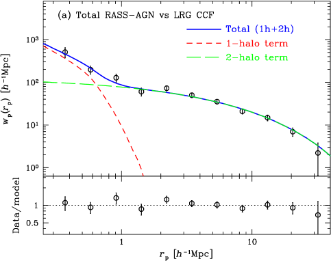
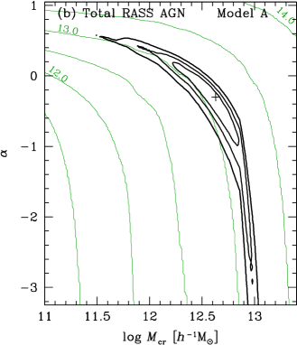
Figure 2.— (a) The AGN-LRG CCF (for the total RASS-AGN sample) and our best-fit HOD model for Model A. The symbols and line styles are the same as in Fig. 1(a). (b) The confidence contours of the Model A parameters ($\log\,\,M_{\rm cr}$,$\alpha$). The confidence contours (thick contours) are at the $\Delta\chi^{2}=1.0,2.3$ and $4.6$ levels. The thin-contours (green) show the mean halo mass $\log\,\langle M_{\rm h}[h^{-1}{\rm M_{\sun}}]\rangle$ derived from the model parameters. Every other contour level is labeled. The contours show that the parameter constraints are almost along a constant $\log\,\langle M_{\rm h}\rangle$ line.

Using the methods described above, we obtain constraints on the AGN HOD parameters $\log\,M_{\rm cr}$ and $\alpha$ in Eq. 17. For each point in this two parameter space, we can also calculate the mean dark matter halo mass occupied by the AGN sample,

$$\langle M_{\rm h}\rangle=\frac{\int M_{\rm h}\langle N_{\rm A}\rangle(M_{\rm h})\phi(M_{\rm h})dM_{\rm h}}{\int\langle N_{\rm A}\rangle(M_{\rm h})\phi(M_{\rm h})dM_{\rm h}},$$ (19)

as well as the effective bias parameter of AGNs $b_{\rm A}$ (Eq. 12).

Figure 2(a) compares our AGN-LRG CCF for the total RASS-AGN sample and our best-fit model.

Figure 2(b) shows the confidence contours in the $\log\,M_{\rm cr}$ – $\alpha$ space, overlaid on underlying thin (green) contours showing the mean halo mass $\langle M_{\rm h}\rangle$. A line of constant bias, $b_{\rm A}$, roughly follows a constant $\langle M_{\rm h}\rangle$ contour, with small deviations caused by the non-linearity of the $b_{\rm h}(M_{\rm h})$ function. The degree of the deviation is such that $\log\langle M_{\rm h}\rangle$ for a given $b$ decreases typically by $\approx 0.4$ when $\alpha$ is decreased from $\approx 1$ to $\approx-3$. Figures 3 and 4 show our HOD fits and confidence contours, respectively, for the high $L_{\rm X}$ and low $L_{\rm X}$ RASS-AGN samples, with an emphasis on the comparison between the two.

Figures 2(b) and 4 show that the parameter pair $(\log\,M_{\rm cr},\alpha)$ is tightly constrained roughly along the constant $\langle M_{\rm h}\rangle$ line. This primary constraint comes from the amplitude of the 2-halo term, which is proportional to the bias parameter of the AGN sample (for the fixed bias of the LRG sample). In the HOD analysis, however, the inclusion of the 1-halo term adds additional constraints in the two-parameter space.

In any of the total, high $L_{\rm X}$ and low $L_{\rm X}$ RASS-AGN samples, models where the number occupation of AGNs is proportional to $M_{\rm h}$ above $M_{\rm cr}$ ($\alpha=1$) are excluded, while a constant number of AGNs per halo above $M_{\rm cr}$ is preferred. Figs 2(b) and 4 put constraints on the values of $M_{\rm cr}$ for each sample. Using the $\Delta\chi^{2}=2.3$ contour (68% confidence level for two parameters), the minimum mass is constrained to be $\log\,M_{\rm cr}[h^{-1}{\rm M}_{\sun}]\gtrsim$ 11.9, 11.9, & 10.7 for the total, high $L_{\rm X}$ and low $L_{\rm X}$ RASS-AGN samples respectively. For the total RASS-AGN sample, the contour is constrained to have $\alpha>-3.0$, while for the high $L_{\rm X}$ and low $L_{\rm X}$ RASS-AGN samples, the contour allows the smallest $\alpha$ that we have explored ($\alpha=-3.25$). This essentially gives constraints on the width of the HOD, and at least for the total RASS-AGN sample, a delta-function type HOD could be marginally excluded.

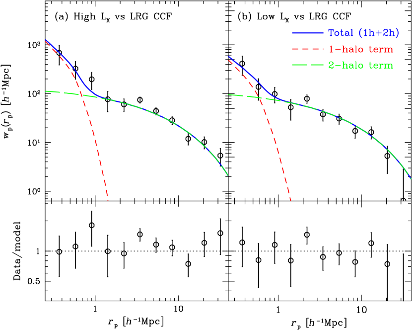
Figure 3.— The AGN-LRG CCFs and the best-fit HOD models (Model A) for the (a) high $L_{\rm X}$ and (b) low $L_{\rm X}$ RASS-AGN samples. The meanings of line styles and symbols are the same as those in Fig. 2(a).

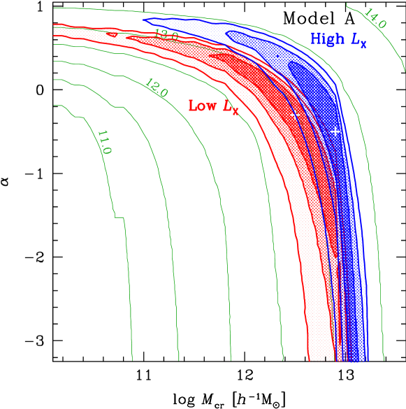
Figure 4.— The confidence contours of the fits to the CCFs to Model A for the high $L_{\rm X}$ (thick blue lines) and the low $L_{\rm X}$ (thick red lines) RASS-AGN samples. The contours are at $\Delta\chi^{2}=1.0,2.3$ and $4.6$ levels. The confidence contours are shaded for the ease of the visibility of the difference between the two samples. The $\log\,\langle M_{\rm h}\rangle$ contours are shown in the same way as in Fig. 2(b).

Table 2The HOD parameters for RASS AGNs at $z\approx 0.28$ (Model A)

RASS-AGN	$\log M_{\rm cr}$	$\alpha$	$\langle N_{\rm A}\rangle(M_{\rm cr})$	$\log\,\langle M_{\rm h}\rangle$	$b_{\rm A}$	$\chi^{2}$
Sample	[$h^{-1}{\rm M}_{\sun}$]			[$h^{-1}{\rm M}_{\sun}$]
Total	12.6 (11.9; 13.0)	-0.3 (0.4;-3.0)	8$\times 10^{-2}$	13.09$\pm$0.08	1.30$\pm$0.09	6.9
High $L_{\rm X}$	12.9 (11.9; 13.2)	-0.5 (0.7;-3.25)	3.3$\times 10^{-3}$	13.26${}^{+0.07}_{-0.09}$	1.44${}^{+0.04}_{-0.11}$	10.9
Low $L_{\rm X}$	12.5 (10.7; 13.0)	-0.3 (0.7;-3.25)	5.5$\times 10^{-2}$	12.97${}^{+0.17}_{-0.13}$	1.22$\pm$0.15	12.5

The best fit HOD parameters, the mean DMH mass occupied by the AGNs, and the linear bias from the fits are summarized in Table 2. For the fitting parameters $\log\,M_{\rm cr}$ and $\alpha$, we show the full range corresponding to 68% confidence range in the 2D parameter space ($\Delta\chi^{2}=2.3$). As shown in Figs. 2 and 4, these two parameters are highly correlated and the confidence contours are skewed, thus one should be cautious in interpreting these ranges. On the other hand, if we project the probability distribution on the variable $\langle M_{\rm h}\rangle$ or the variable $b$ (bias), both of which are unique functions of our two fitting parameters, the projected probability distribution becomes roughly Gaussian. Thus we take the $\Delta\chi^{2}<1$ range (68% error for one parameter) to estimate the 1$\sigma$ errors of these derived quantities, $\langle M_{\rm h}\rangle$ and $b_{\rm A}$, in Table 2.

We note that because of the exponential drop of the DMH mass function the HOD at very high $M_{\rm h}$ contributes little to the CCF. In order to check the maximum $M_{\rm h}$ that our analysis can reasonably constrain, we recalculate the CCF with the truncated power-law model with an upper mass cutoff:

$$\langle N_{\rm A}\rangle\propto M_{\rm h}^{\alpha}\;\Theta(M_{\rm h}-M_{\rm cr})\Theta(M_{\rm cut}-M_{\rm h})$$

We recalculate $\chi^{2}$ with varying $M_{\rm cut}$ while fixing ($M_{\rm cr}$,$\alpha$) at the best-fit value above. The change of $\chi^{2}$ from the $M_{\rm cut}=\infty$ is larger than unity at $\log M_{\rm h}[h^{-1}M_{\sun}]<14.0$. Thus our HOD analysis is sensitive up to $M_{\rm h}\approx 10^{14}h^{-1}M_{\rm\sun}$, i.e., the mass of a poor cluster.

4.2. HODs and Space Densities

In order to illustrate the range of acceptable HODs, we plot a number of representative AGN HOD models accepted by our fits ($\langle N_{\rm A}\rangle(M_{\rm h})$) as function of DMH mass in Fig. 5(a). In Fig. 5(b), we also show the same sets of models in units of the spatial density per comoving volume per log of the DMH mass:

$$\langle N_{\rm A}\rangle(M_{\rm h})\frac{d\phi(M_{\rm h})}{d\log\,M_{\rm h}}\equiv\langle N_{\rm A}\rangle(M_{\rm h})\cdot\ln(10)M_{\rm h}\phi(M_{\rm h}).$$ (20)

These models have been normalized to the observed number densities (see Table 1). In each panel, three curves are plotted, representing the best-fit case and two extreme cases. These are (1) for the best-fit values (solid lines), (2) the point on the $\Delta\chi^{2}=2.3$ contour that has the smallest $M_{\rm cr}$ value (i.e., the upper left tip of the two-parameter 68% confidence area in Fig. 2(b) or 4) (dotted lines), and (3) the smallest $\alpha$ point on the $\Delta\chi^{2}=2.3$ (the bottom of the confidence region and narrowest possible HOD distribution, dashed lines). The best-fit model with $\alpha=-3.25$ (the smallest $\alpha$ in our search grid) is used for the high $L_{\rm X}$ and low $L_{\rm X}$ RASS-AGN samples, for which the $\Delta\chi^{2}=2.3$ contour continues below $\alpha=-3.25$. These three models have been plotted to illustrate the almost full range of possible HODs statistically accepted by our analysis. In order to illustrate the DHM mass range that can be occupied by both LRGs and AGNs, and therefore contributes to the 1-halo term of the CCF, we also show the HODs of the LRGs for reference. Of course, these plots are for our rather restrictive truncated power-law model and by no means are intended to illustrate an exhaustive set of possible HODs. However, this illustrates that these three models have roughly the same average $M_{\rm h}$, with varied widths of the HOD. An important constraint is that the AGN HOD can be no wider than the dotted line in 5(a)(b), which represents the point corresponding to the lowest extreme of $M_{\rm cr}$ and the roughly highest extreme of $\alpha$, among acceptable models with $\Delta\chi^{2}<2.3$. The meaning of this constraint is discussed in Sect. 5.2.

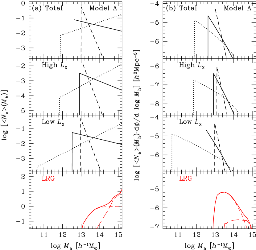
Figure 5.— (a) The HODs ($\langle N_{\rm A}\rangle(M_{\rm h})$) of Model A for three representative points in the parameter space that are acceptable ($\Delta\chi^{2}<2.3$) from our fits for each of the total (top panel), high $L_{\rm X}$ (upper middle panel) and low $L_{\rm X}$ (lower middle panel) AGN samples. The solid, dotted, and dashed lines represent the (1) best-fit, (2) lowest $M_{\rm cr}$ extreme, and (3) lowest $\alpha$ extreme respectively (see text). For reference, the bottom panel shows the LRG HODs for the central galaxies (short-dashed line), satellites (long-dashed line), and their sum (solid line). (b) The same set of models are shown in terms of the spatial number density per $\log\,M_{\rm h}$. The meaning of the line styles is the same as those in panel (a).

4.3. Effects of Central AGNs

In this section we explore models in which central AGNs are explicitly included, using galaxy HODs as a template. Galaxy HODs have been extensively investigated using, e.g., SDSS data, with a high statistical accuracy. A simple model for luminosity-threshold galaxy samples (i.e. more luminous than a given limit), introduced by (Zehavi et al. 2005a) is a three parameter model including a step function for the central HOD and a truncated power-law satellite HOD. We express the AGN HODs here with the same form, except that the global normalization is also a free parameter (Model B):

$$\langle N_{\rm A,c}\rangle = f_{\rm A}\Theta(M_{\rm h}-M_{\rm min}),$$

$$\langle N_{\rm A,s}\rangle = f_{\rm A}\Theta(M_{\rm h}-M_{\rm min})(M_{\rm h}/M_{1})^{\alpha_{\rm s}},$$ (21)

where $f_{\rm A}$ is the AGN fraction (duty cycle) among central galaxies at $M_{\rm h}\gtrsim M_{\rm min}$. We use the symbol $\alpha_{\rm s}$ to emphasize that it represents the HOD slope for satellites. $M_{1}$ is the DMH mass at which the number of central AGNs is equal to that of satellite AGNs. For luminosity-threshold galaxy samples, it is usually assumed that the central galaxy HOD saturates at unity at the high $M_{\rm h}$ end (i.e., $f_{\rm A}=1$ in Eq. 21), because central galaxies in the highest mass DMHs are expected to be luminous enough to be included in the sample (e.g. Sect. 3.2.1). Since only a small fraction of galaxies contain an AGN, this has to be multiplied by a factor $f_{\rm A}(<<1)$, the value of which does not affect the CCF as discussed above. The value of $f_{\rm A}$ can be determined by normalizing the HOD to $n_{\rm AGN}$.

It is important to note the underlying physical assumption of Eq. 21, which is that the AGN duty cycle among central galaxies does not depend on the DMH mass. We explore the consequences of this model as an illustrative contrast to Model A, which assumes a suppression of the AGN duty cycle in central galaxies of high mass DMHs.

We investigate the behavior of $\chi^{2}$ (Eq. 18) in the space of $M_{\rm min}$, $M_{1}$, and $\alpha_{\rm s}$. Due to the low signal-to-noise ratio of the CCFs for our luminosity-divided subsamples, we limit our discussion to the total sample. Even with the total sample, our statistics do not allow us to constrain all three parameters; therefore we investigate the constraints on two parameters by fixing the remaining parameter. The HOD analysis of luminosity-threshold samples with $-21.5\leq M_{r}^{\rm max}\leq-21.0$, studied by Zehavi et al. (2005a) found $M_{1}/M_{\rm min}\approx 23$ and $\alpha_{\rm s}\approx 1.2$. We consider the typical HOD of SDSS galaxy samples in this luminosity threshold range as a template because their $M_{\rm min}$ range ($12.0\lesssim\log M_{\rm min}[h^{-1}M_{\sun}]\lesssim 12.7$) roughly coincides with the minimum DMH range for our AGNs, as we see from the range of $M_{\rm cr}$ in the confidence contour in Fig. 2(b), which approximately coincide with the range of $M_{\rm min}$ as we see below. We therefore (i) fix $M_{1}/M_{\rm min}=23$ and obtain constraints in the $(\log\,M_{\rm min},\alpha_{\rm s})$-space, and (ii) fix $\alpha=1.2$ and obtain constraints in the $(\log\,M_{\rm min},M_{1}/M_{\rm min})$-space.

Figure 6.— (a) The confidence contours of the Model B parameters in the ($\log\,\,M_{\rm min}$,$\alpha_{\rm s}$) space for $M_{1}/M_{\rm min}=23$. (b) The confidence contours of the same set of parameters for Model C, for $\log M_{\rm cc}[h^{-1}M_{\sun}]=13.0$ and $M_{1}/M_{\rm min}=23$. The contours are at $\Delta\chi^{2}=1.0,2.3$ and $4.6$ levels.

Table 3The HOD parameters for the RASS AGNs (Models B & C)

Model	RASS-AGN	$\log M_{\rm min}$	$M_{\rm cc}$	$\log M_{1}/M_{\rm min}$	$\alpha_{\rm s}$	$f_{\rm A}$	$\chi^{2}$
	Sample	[$h^{-1}{\rm M}_{\sun}$]	[$h^{-1}{\rm M}_{\sun}$]
B	Total	12.5 (12.2;13.0)	…	1.36 (fixed)	0.55 (0.95;-1.50)	2.9$\times 10^{-2}$	6.9
B	Total	12.4 (11.9;12.6)	…	1.65 (1.51;1.83)	1.20 (fixed)	3.3$\times 10^{-2}$	8.4
B	Total	12.3 (12.1;12.7)	…	1.55 (1.36;1.81)	1.00 (fixed)	2.6$\times 10^{-2}$	7.7
C	Total	12.6 (12.2;13.0)	13.0 (fixed)	1.36 (fixed)	0.0 (0.84;-1.50)	3.7$\times 10^{-2}$	6.8

The resulting confidence contours for (i) are shown in Fig. 6(a). The best-fit parameters and $\chi^{2}$ values are summarized in Table 3 for both (i) and (ii), where we also show the $\alpha_{\rm s}=1.0$ case for (ii), in which the number of satellites is proportional to the DMH mass.

For the $M_{1}/M_{\rm min}=23$ case, the best-fit slope for the satellite is below unity ($\alpha_{\rm s}=0.55$) and $\chi^{2}=6.9$ is identical to that of Model A. The best-fit model with $\alpha_{\rm s}=1.0$ is marginally rejected ($\Delta\chi^{2}=3.6$) and the model with $\alpha_{\rm s}=1.2$ is significantly rejected ($\Delta\chi^{2}=18$). Models that are consistent with $\alpha_{\rm s}=1.2$ can be found at $M_{1}/M_{\rm min}\geq 30$, but they are not consistent with the HOD of luminosity threshold galaxy samples in the $-21.5\leq M_{r}^{\rm max}\leq-21.0$ range.

We also explore a model (Model C) where only lower mass DMHs contain a central AGN, where the physical picture is explained at the introduction of Model A (Sect. 3.2.2). In this model, the central HOD in Model B is replaced by

$$\langle N_{\rm A,c}\rangle=f_{\rm A}\Theta(M_{\rm h}-M_{\rm min})\Theta(M_{\rm cc}-M_{\rm h}),$$ (22)

while the form of $\langle N_{\rm A,c}\rangle$ stays the same. As a representative case, we choose $\log M_{\rm cc}[h^{-1}M_{\sun}]=13.0$, below which the DMH center is more frequently occupied by blue galaxies than red galaxies in the HOD analysis of color-separated samples by Zehavi et al. (2005a), while we keep $M_{1}/M_{\rm min}=23$ (but see also Zehavi et al. (2010), which use a different parametrization on color-separated samples). The confidence contours are shown in Fig. 6(b) and the best-fit parameters and $\chi^{2}$ values are shown in Table 3. In this scenario, the best-fit slope for the satellite is $\alpha_{\rm s}=0$, while $\alpha_{\rm s}=1.0$ is rejected at the $\Delta\chi^{2}=4.8$ level.

5. Discussion

5.1. Comparison with Results from Paper I

Table 4Comparion of Results from Paper I

(1)	(2)	(3)	(4)	(5)	(6)	(7)	(8)
RASS-AGN	$b_{\rm A}$	$b_{\rm A}$	$b_{\rm A}$	$\log\langle M_{\rm h}\rangle$	$\log(M_{\rm h,typ})$	$\log(M_{\rm h,typ})$	$\log(M_{\rm h,typ})$
Sample	HOD	PL	PL,$>1.5$	HOD,tin05	HOD,tin05	PL,smt01	PL,tin05
				[$h^{-1}{\rm M}_{\sun}$]
Total	1.32$\pm$0.08	1.11${}^{+0.10}_{-0.12}$	1.52$\pm 0.21$	13.09$\pm$0.08	13.00$\pm$0.12	12.58${}^{+0.20}_{-0.33}$	12.70${}^{+0.19}_{-0.30}$
High $L_{\rm X}$	1.44${}^{+0.04}_{-0.11}$	1.44${}^{+0.22}_{-0.27}$	1.56 $\pm 0.23$	13.26${}^{+0.07}_{-0.09}$	13.19${}^{+0.05}_{-0.12}$	13.10${}^{+0.24}_{-0.43}$	13.27${}^{+0.22}_{-0.41}$
Low $L_{\rm X}$	1.23$\pm$0.15	0.88${}^{+0.14}_{-0.17}$	1.6${}^{+2.1}_{-0.6}$	12.97${}^{+0.17}_{-0.13}$	12.87${}^{+0.13}_{-0.30}$	11.83${}^{+0.55}_{-\infty}$	12.03${}^{+0.39}_{-1.48}$

Table 4 compares our results with those from paper I. The meanings of the table columns are: (1) sample, (2) the bias parameter from the HOD analysis (Eq. 12), (3) the bias parameter from paper I, i.e. for the power-law fit in $0.3<r_{\rm p}[h^{-1}{\rm Mpc}]<15$, (4) the bias parameter for the power-law fit in $1.5<r_{\rm p}[h^{-1}{\rm Mpc}]<15$ calculated in the same way as paper I (see below), (5) the “mean” DMH mass from Eq. 19, (6) the “typical” DMH mass calculated from $b_{\rm A}$ from the HOD model, defined by $b_{\rm h}(M_{\rm typ})=b_{\rm A}$ calculated with the $b_{\rm h}(M_{\rm h})$ by Tinker et al. (2005) (see Sect. 3.1). (7) the “typical” DMH mass from paper I (i.e. from power-law fits) calculated with the $b_{\rm h}(M_{\rm h})$ by Sheth et al. (2001), and (8) the “typical” DMH mass from the paper I bias parameter re-calculated using the $b_{\rm h}(M_{\rm h})$ relation by Tinker et al. (2005). While the results from the the HOD analysis presented here and the simple analysis of paper I agree well for the high $L_{\rm X}$ RASS-AGN sample, the HOD analysis gives larger bias parameters than those derived in paper I for the total and low $L_{\rm X}$ RASS-AGN samples at the level of 1.5 $\sigma$. Since these bias parameters have been derived from the same dataset with different methods, the discrepancies are systematic rather than statistical. One of the major findings of paper I is the detection of the X-ray luminosity dependence of the correlation function. The difference in correlation lengths ($r_{0}$), between the high $L_{\rm X}$ and low $L_{\rm X}$ RASS-AGN samples measured in paper I is $\approx 2.5\sigma$, based on power-law fits with a fixed slope of $\gamma=1.9$. The differences of the AGN bias parameters $b_{\rm A}$ and associated typical DMH mass $M_{\rm h,typ}$ derived from power-law fits are $\approx 1.8\sigma$. In the HOD analysis, the significance of the difference in $b_{\rm A}$ decreases to $1.1\sigma$, because it is constrained mainly by measurements at large scales where the 2-halo term dominates (see below). However, in terms of $M_{\rm h,typ}$ derived from the HOD analysis, the difference is $\approx 1.8\sigma$ because of the additional constraints from the 1-halo term.

There are a number of differences in the processes used to derive the bias parameter between paper I and this work. In paper I, the bias parameters are based on the power-law fits to Eq. 3 over scales of $0.3<r_{\rm p}[h^{-1}{\rm Mpc}]<15$, assuming a linear bias over the entire scale range. Then the power-law models are converted into the rms fluctuations over 8 $h^{-1}$ Mpc spheres ($\sigma_{\rm 8,AGN}$), and the bias parameter is calculated using $\sigma_{\rm 8,AGN}/[\sigma_{0}D(z)]$, where $D(z)$ is the linear growth factor. The main source of discrepancy is that, while paper I also uses data points down to a scale of $r_{\rm p}=0.3h^{-1}$ Mpc to obtain $b$, in the HOD analysis presented here the constraints on $b$ mainly come from the 2-halo term dominated region ($r_{\rm p}\gtrsim 1.5h^{-1}$), while smaller scale data constrain other variables. Fig. 3 shows that the difference between the high $L_{\rm X}$ and low $L_{\rm X}$ RASS-AGN samples is more prominent in the 1-halo term dominated regime, at $r_{\rm p}\lesssim 1h^{-1}$, than in the 2-halo term dominated regime. This means that, for the AGN-LRG CCF, the 1-halo term is more sensitive to differences in the AGN HOD. The reason for this is that while $b_{\rm h}(M_{\rm h})$ increases only weakly with increasing with $M_{\rm h}$, the 1-halo term is directly proportional to the number of AGNs that are in the same DMHs as those occupied by LRGs, i.e., very massive ones ($\log M_{\rm h}\gtrsim 13.5[h^{-1}{\rm M_{\sun}}]$), i.e. the 1-halo term is more sensitive to the existence of AGNs in high mass halos.

In the literature, relative or absolute bias parameters are often calculated based on results from power-law fits (e.g., paper I; Mullis et al. 2004; Yang et al. 2006; Miyaji et al. 2007; Coil et al. 2009). The power-law models of $\xi(r)$ are usually converted to the rms fluctuation over 8$h^{-1}$ Mpc spheres or are averaged up to the distance of 20$h^{-1}$ Mpc ($\bar{\xi}(<20h^{-1}{\rm Mpc})$). While some authors use only large scales ($r_{\rm p}>1-2h^{-1}$Mpc) to ensure that only the linear regime is used, others include smaller scales. Usually the rationale for including smaller scales is to have better statistics, combined with the empirical observation that the correlation functions are well fit with a power-law model over the scale of $0.1-0.3\lesssim r_{\rm p}\lesssim 10-20h^{-1}$Mpc ($0.3<r_{\rm p}<15h^{-1}$ Mpc in the case of paper I). As a check, we have re-calculated the bias parameter for power-law fits to the $w_{p}(AGN|AGN)$ used in Paper I on scales of $1.5<r_{\rm p}<15h^{-1}$ Mpc, to limit ourselves to the linear regime. These are shown in column (4) of Table 4. The bias parameters obtained in this manner carry large statistical errors, but the values are consistent with those derived from the HOD analysis within 1$\sigma$ in all three samples, while they are more than $\approx 1\sigma$ above the bias parameters derived in paper I for the total and low $L_{\rm X}$ RASS-AGN samples. The AGN bias parameters in our total and high $L_{\rm x}$ samples from the HOD analysis, as well as the power-law fit $1.5<r_{\rm p}<15h^{-1}$ Mpc, are consistent within combined 1$\sigma$ errors with those measured by Padmanabhan et al. (2009) for their QSO samples ALL0 and LSTAR0, which covers a similar redshift range as ours ($0.25<z<0.35$). However, their bias parameters for their higher redshift QSO samples, ALL1 & LSTAR1 ($0.33<z<0.50$) as well as ALL2 & LSTAR2 ($0.45<z<0.60$) are lower.

Using the power-law fit results including the non-linear regime is useful to detect the different clustering properties between, e.g., different source populations, luminosities, or types. In our case, this gives the most statistically significant difference between the clustering properties of the high $L_{\rm X}$ and low $L_{\rm X}$ RASS-AGN samples. However, one has to be careful in interpreting the results, e.g., in terms of the DMH mass based on the bias parameter. In principle, the HOD analysis overcomes this limitation, because we are able to derive the pure linear bias parameter, while at the same time utilizing the data in the non-linear regime.

5.2. Implications for the Environments of AGN Accretion

With the HOD analysis, we can also obtain constraints on at least one additional variable which is independent from the “mean” DMH mass, thanks to the constraints from the 1-halo term. The importance of the 1-halo term constraints has also been noted by Padmanabhan et al. (2009) using a similar CCF analysis between photometric-redshift LRG samples and optically-selected QSOs in SDSS at $z\sim 0.5$. They qualitatively concluded that at least some QSOs must be satellites and also that models of the form of our Model B (Eq. 21) with $M_{1}/M_{\rm min}=20$ and $\alpha_{\rm s}=0.9$ are also acceptable, while lower $\alpha$ values are also possible. Our analysis here gives qualitatively similar results.

The acceptable parameter space for Model A is always in the $\alpha<1$ regime for all of our three AGN samples: the total, high $L_{\rm X}$, and low $L_{\rm X}$ RASS-AGN samples. This means that the average number of AGNs in a DMH does not increase proportionally with mass. Figs. 2(b) and 4 show that models with $\alpha\lesssim 0$ are preferred. It is interesting to compare this result with HOD analyses of galaxies, that find $\alpha_{\rm s}\approx 1-1.2$ for a wide range of absolute magnitudes and redshifts at least up to $z\approx 1.2$ (Zehavi et al. 2005a; Zheng et al. 2007; Zehavi et al. 2010). In principle, neither the results nor the assumptions of Model A say anything about the central fraction among AGNs at the lower mass DMHs (see Sect. 3.2.2), and thus they do not directly constrain the slope of the satellite AGN HOD $\alpha_{\rm s}$. However, if we take the extreme case where all the AGNs are satellites, $\alpha_{\rm s}<0.4$, this would imply that AGN fraction among satellite galaxies strongly decrease with $M_{\rm h}$. In Model B, where the central galaxy component is included explicitly under the assumption that the AGN duty cycle in central galaxies is constant against varying $M_{\rm h}$ above $M_{\rm min}$, the best-fit slope is still less than unity ($\alpha_{\rm s}=0.55$), and models with $\alpha_{\rm s}\approx 1$ are only marginally rejected for $M_{1}/M_{\rm min}=23$ (a representative value of luminosity-threshold galaxy samples). In case of Model C, where only $\log\,M_{\rm h}[h^{-1}M_{\sun}]<13.0$ DMHs can contain a central AGN, the best-fit solution is $\alpha_{\rm s}=0$, while $\alpha_{\rm s}\approx 1$ is rejected at a $\sim 2\sigma$ level for $M_{1}/M_{\rm min}=23$. On the whole, our results tend to favor models in which the AGN fraction among satellite galaxies decreases with increasing DMH mass (or the richness of groups and clusters), in the mass range $12-13\lesssim\log\,M_{\rm h}[h^{-1}{\rm M_{\sun}}]\lesssim 14.0$.

Since our AGN sample is selected from X-ray point sources in RASS, and since clusters of galaxies (which represent the most massive DMHs) are also X-ray sources, an observational bias that might affect our results is that AGNs in the clusters are selected against in the RASS-AGN sample due to confusion, especially considering that the mean point spread function (PSF) has a FWHM$\approx 2$ arcminutes (La Barbera et al. 2009), which is not negligible when compared to the extent of the cluster X-ray emission. We have estimated the significance of this effect as follows. The detection limit of the cluster diffuse X-ray emission is higher than that of point sources. A typical flux limit for clusters in RASS is $S_{\rm X}\approx 2\times 10^{-12}$ erg s^-1 cm^-2, (0.1-2.4 keV)(Böhringer et al. 2001; Popesso et al. 2004), corresponding to $\log\,L_{\rm X}\gtrsim 44.3$ $[h_{70}^{-2}{\rm erg\,s^{-1}}]$ at the lower bound of our redshift range of $z\approx 0.16$. This scales to a cluster virial mass of $\log\,M_{\rm h}\gtrsim 14.5\,h^{-1}{\rm M_{\sun}}$ (Reiprich & Böhringer 2002). As we found at the end of Section 4.1, our CCF is only sensitive to the HOD behavior at $\log\,M_{\rm h}\lesssim 14.0\,h^{-1}{\rm M_{\sun}}$, and thus this selection effect should play negligible role in our results. Additionally, a confusion due to two or more X-ray AGN point sources being artifically blended into a single source by the RASS point spread function (PSF) is not important either, as $\langle N_{\rm A}\rangle$ is much less than unity over all masses (see Fig. 5). Thus we can state with a good degree of confidence that our limits on $\alpha$ (Model A) or $\alpha_{\rm s}$ (Model B/C) are not an artifact of X-ray source confusion.

Our results of $\alpha_{\rm s}<1$, found in our extensive explorations in the parameter space of the models that we consider, may be interpreted in view of the long-suggested deficiency of emission line diagnostic-selected AGNs in rich clusters (e.g. Gisler 1978; Dressler et al. 1985). While our CCF analysis is not sensitive to rich clusters (Sect. 4.1), a more recent work by Popesso & Biviano (2006) verified that this trend extends to the group scale by finding an anti-correlation between AGN fraction and the galaxy velocity dispersion in nearby ($z<0.08$) groups/clusters of galaxies down to the velocity dispersion of $\sigma_{\rm v}\sim 200\,[{\rm km\,s^{-1}}]$. Arnold et al. (2009) also found that the X-ray selected AGN ($\log\,L_{\rm X}\gtrsim 41h_{70}^{-1}$erg s^-1, representing a much lower luminosity population than our AGNs) fraction is larger in groups than in clusters by a factor of two at low redshifts ($0.02<z<0.06$). Various physical mechanisms have been suggested to explain the deficiency of star-formation galaxies in clusters of galaxies, and similar processes might be responsible for the lack of AGNs as well. These include ram-pressure stripping (Gunn & Gott 1972) or evaporation (Cowie & Songaila 1977) of a galaxy’s interstellar medium, which is a required ingredient of the AGN activity in galaxies, by the hot intracluster medium. Also, if AGN activity is triggered by mergers between two gas-rich galaxies, another possible mechanism for this trend is the decreased cross-section for galaxy mergers in the galaxy-galaxy close encounters at high relative velocities (Makino & Hut 1997). In high mass DMHs, representing richer groups/clusters, the velocity dispersion is higher and thus one may expect that there are fewer mergers than in groups of galaxies (Popesso & Biviano 2006), although the density of galaxies increase at the center. Other mechanisms such as the accretion of small gas-rich dwarf galaxies (minor mergers) may play a role in fueling the AGN host, but it is not clear how this would affect the slope $\alpha_{\rm s}$.

In order to fully understand the growth history of SMBHs as well as the physical processes responsible for the AGN activity in groups and clusters, we need to explore the statistics at different redshifts, luminosities, and AGN types. The results mentioned above that investigate AGNs in groups/clusters are concerned with AGN at lower redshifts and with lower luminosities than the AGNs in our CCF analysis. In the AEGIS field, Georgakakis et al. (2008) found that AGNs at $z\approx 1$ are more frequently found in the group environment than the overall galaxy population. However, deep field surveys such as AEGIS do not contain a large enough volume to explore the richness dependence of the AGN fraction in groups/clusters. Martini et al. (2009) investigate Chandra images of a sample of 33 clusters at $0.05<z<1.3$, finding that the luminous AGN ($\log\,L_{\rm X}\gtrsim 43h_{70}^{-1}$erg s^-1) fraction increases with redshift. They explore the redshift dependence of the AGN fraction, but not the richness dependence. At $z<0.4$, where the luminosity range of their AGNs is closer to ours, they have only two AGNs in 17 clusters in the redshift range that is similar to our sample. A much larger sample of groups/clusters is needed to explore the richness dependence of the AGN fraction in a sufficiently narrow redshift range to avoid any degeneracy with the redshift dependence.

In general, directly investigating AGN prevalence in individual groups and clusters is observationally and analytically intensive. The HOD analysis of galaxy-AGN CCF provides a strong statistical tool with which to probe the AGN population in groups and clusters, which can be made without identifying individual groups and clusters. Thus it is important to extend the HOD analysis to AGN clustering measurements at higher redshift, especially in view that the fraction of star-forming galaxies in clusters increase with redshift (Butcher & Oemler 1984). It is also important to have larger numbers of AGNs for the CCF measurements, which will enable measurements of small-scale clustering and produce stronger constraints on $\alpha_{\rm s}$, as well as to break the model degeneracy. Using non-LRG galaxies for the CCF to obtain the 1-halo term constraints in the lower $M_{\rm h}$ regime would also improve the analysis.

Linked to our constraints on $\alpha$ in Model A, we also have weak constraints on the range of $M_{\rm cr}$. The range of $M_{\rm cr}$ is similar to that of $M_{\rm min}$ in Model B. Using the scaling relations and the luminosity range of our RASS-AGN samples, we can make an interesting comparison. Figure 1 of paper I shows that the minimum 0.1-2.4 keV luminosities of the total and high $L_{\rm X}$ RASS-AGN samples are $\log\,L_{\rm X}\,[h_{70}^{-2}{\rm erg\,s^{-1}}]\approx 43.7$ & 44.3 respectively, while the low $L_{\rm X}$ sample has the same minimum luminosity as the total RASS-AGN sample. Converting the 0.1-2.4 keV luminosity to a 0.5-2 keV luminosity, assuming a power-law spectrum with photon index $\Gamma=2.5$ and applying the luminosity-dependent bolometric correction from Eq. (2) of Hopkins et al. (2007), the corresponding bolometric luminosities are $\log\,L_{\rm bol}\,[h_{70}^{-2}{\rm erg\,s^{-1}}]\approx$ 44.5 and 45.4 for the total and high $L_{\rm X}$ RASS-AGN samples. The mass of the SMBH ($M_{\bullet}$) corresponding to the minimum luminosity is then $M_{\bullet}\approx 2\times 10^{6}/\lambda$ and $2\times 10^{7}/\lambda$ $[{\rm M_{\sun}}]$, where $\lambda\equiv L_{\rm bol}/L_{\rm Edd}$ and $L_{\rm Edd}$ is the Eddington Luminosity.

The relation between the black hole mass $M_{\bullet}$ and the DMH of its host galaxy is explored by Ferrarese (2002) by comparing the rotation curves of spiral galaxies. While their $M_{\bullet}$-DMH mass relation is subject to uncertainties due to different assumptions of the circular velocity and virial velocity by a factor of a few, using their Eq. (6) with Bullock et al. (2001)’s recipe, the above black hole mass corresponds to a galaxy halo mass of $4\times 10^{11}$ ($1.5\times 10^{12}$) $\cdot\lambda^{-0.6}[{\rm M_{\sun}}]$ (for $h=0.7$). These masses are comparable or slightly lower than the lower bounds of $M_{\rm cr}$ derived above for those AGNs emitting at the Eddington luminosity and are an order of magnitude lower than our best-fit values. In general, the concept of the DMH of a galaxy explored by Ferrarese (2002) is different from the DMH derived in our CCF/HOD analysis, since the large-scale correlation function reflects the DMH mass as the largest virialized structure the object belongs to. If the largest virialized structure represents a group or cluster of galaxies, then there are multiple objects in a DMH, and the DMH that is related to Ferrarese (2002)’s scaling relation represents a sub-halo in a larger mass halo. While our statistics do not allow for strong constraints, if $M_{\rm cr}$ is close to our nominal value, then the lowest luminosity AGNs among our samples should be accreting at a sub-Eddington rate ($\lambda<0.1$) or reside in groups.

6. Conclusion

We have applied a halo occupation distribution (HOD) model to the two-point cross-correlation function (CCF) between broad-line RASS-AGN and luminous red galaxies (LRGs) at $0.16<z<0.36$ measured in paper I. We have developed a method of applying the HOD model directly to the CCF, where we have used the well-determined HOD of the LRG as a reference to constrain the HOD of the AGNs. Our findings are summarized as follows:

1. From our HOD analysis of the AGN-LRG CCF, we have found constraints on the HOD of AGNs. We have modeled the AGN HOD as a truncated power-law model (Model A) with two parameters: the critical dark matter halo (DMH) mass ($M_{\rm cr}$) below which the AGN HOD is zero (i.e, there are no AGN in halos below this mass threshold), and the slope $\alpha$, where the HOD $\propto M_{\rm h}^{\alpha}$ for $M_{\rm h}\geq M_{\rm cr}$. We have obtained joint constraints in this two-parameter space, $M_{\rm cr}-\alpha$ under the scenario that there is no central AGNs in high mass halos.

2. The constraints in this $M_{\rm cr}-\alpha$ space lie mainly along lines of constant large-scale bias and constant mean DMH mass. These provide a more accurate determination of the mean mass of the DMHs in which AGNs reside than the analysis based on power-law fits provided in Paper I. The mean DMH mass we derive is $\langle M_{\rm h}\rangle[h^{-1}{\rm M_{\sun}}]$ $=13.09\pm 0.08$, 13.26${}^{+0.07}_{-0.09}$, and 12.97${}^{+0.17}_{-0.13}$ for the total, high $L_{\rm X}$ and low $L_{\rm X}$ RASS-AGN samples respectively. The 2-halo term of the CCF primarily constrains the mean DMH mass.

3. In all three of our RASS-AGN samples, we have detected a significant contribution of the 1-halo term in the AGN-LRG CCF, indicating that some AGNs are in the same DMHs occupied by LRGs. This gives additional constraints on the AGN HOD beyond the mean DMH mass.

4. The range of acceptable HODs of high $L_{\rm X}$ and low $L_{\rm X}$ RASS-AGN samples are significantly different in the $M_{\rm cr}-\alpha$ space, confirming the paper I’s results on the X-ray luminosity dependence of AGN clustering properties at the $\approx 2\sigma$ level.

5. The most important constraint we have obtained using Model A is an upper limit (corresponding to $\Delta\chi^{2}=2.3$), of $\alpha\lesssim 0.4$ for the total AGN sample, rejecting $\alpha=1$. In the extreme case where all AGNs are satellites, the results show a sharp contrast with previously derived HODs of galaxies, which show $\alpha\approx 1-1.2$ (i.e., the number of satellite galaxies approximately $\propto M_{\rm h}$), across a range of galaxy luminosity and redshift. Taken at face value, this implies that the AGN fraction among satellite galaxies decreases with increasing $M_{\rm h}$. This is consistent with previous observations that the AGN fraction is smaller in clusters than in groups in the nearby Universe. Possible explanations include the ram-pressure stripping and/or evaporation of galactic gas by the hot intracluster medium and a decreased cross-section for galaxy merging in the high velocity dispersion environment of richer groups/clusters.

6. We also investigated a model (Model B) which is composed of central and satellite AGNs, where the central HOD is constant ($=f_{\rm A}$) and the satellite HOD has a power-law form $=f_{\rm A}(M/M_{\rm 1})^{\alpha_{\rm s}}$, both at masses above $M_{\rm min}$. This model is based on the results of HOD analyses of galaxies. For $M_{1}/M_{\rm min}=23$, which is appropriate for galaxies, we obtain $\alpha_{\rm s}\lesssim 0.95$, finding a marginal preference for a picture in which the AGN fraction among satellite galaxies decrease with DMH mass. With another model (Model C), which has the same form as Model B except that only $\log M_{\rm h}[h^{-1}M_{\sun}]<13.0$ DMHs are allowed to contain a central AGN, we obtain slightly stronger constraints ($\alpha_{\rm s}\lesssim 0.84$) that give preference to this picture.

7. We have also obtained a lower limit (corresponding to $\Delta\chi^{2}=2.3$) of $\log\,M_{\rm cr}[h^{-1}{\rm M_{\sun}}]\lesssim 11.9$ for the total AGN RASS-sample. If the lowest luminosity AGNs in our sample are emitting at the Eddington luminosity, the black hole mass can be scaled to the DMH mass of the galaxy that is comparable to this lower limit of $M_{\rm cr}$. If the critical DMH mass is at the best-fit value ($\log\,M_{\rm cr}\,[h^{-1}{\rm M_{\sun}}]\approx 12.6$), then the lowest $L_{\rm X}$ AGNs in our sample contain SMBHs that accrete at low Eddington ratios and/or reside in group environments.

References

- Aird et al. (2010) Aird, J., et al. 2010, MNRAS, 401, 2531
- Anderson et al. (2003) Anderson, S.F., Voges, W., Margon, B., et al., 2003, AJ, 126, 2209
- Anderson et al. (2007) Anderson, S.F., Margon, B., Voges, W., et al., 2007, AJ, 133, 313
- Arnold et al. (2009) Arnold, T. J., Martini, P., Mulchaey, J. S., Berti, A., & Jeltema, T. E. 2009, ApJ, 707, 1691
- Böhringer et al. (2001) Böhringer, H., et al. 2001, A&A, 369, 826
- Blake et al. (2008) Blake, C., Collister, A., & Lahav, O. 2008, MNRAS, 385, 1257
- Blanton et al. (2005) Blanton, M. R., et al. 2005, AJ, 129, 2562
- Bullock et al. (2001) Bullock, J. S., Kolatt, T. S., Sigad, Y., Somerville, R. S., Kravtsov, A. V., Klypin, A. A., Primack, J. R., & Dekel, A. 2001, MNRAS, 321, 559
- Butcher & Oemler (1984) Butcher, H., & Oemler, A., Jr. 1984, ApJ, 285, 426
- Cappelluti et al. (2010) Cappelluti, N., Ajello, M., Burlon, D., Krumpe, M., Miyaji, T., Bonoli, S., & Greiner, J. 2010, ApJ, 716, L209
- Coil et al. (2007) Coil, A.L., Hennawi, J.F., Newman, J.A, et al. 2007, ApJ, 654, 115
- Coil et al. (2009) Coil, A.L., Georgakakis, A., Newman, J.A., et al. 2009, ApJ, 701, 1484
- Cooray & Sheth (2002) Cooray, A., & Sheth, R. 2002, Phys. Rep., 372, 1
- Cowie & Songaila (1977) Cowie, L. L., & Songaila, A. 1977, Nature, 266, 501
- Davis & Peebles (1983) Davis, M., Peebles, P.J.E., 1983, ApJ, 267, 465
- Dressler et al. (1985) Dressler, A., Thompson, I. B., & Shectman, S. A. 1985, ApJ, 288, 481
- Ebrero et al. (2009a) Ebrero, J., et al. 2009, A&A, 493, 55
- Ebrero et al. (2009b) Ebrero, J., Mateos, S., Stewart, G. C., Carrera, F. J., & Watson, M. G. 2009, A&A, 500, 749
- Eisenstein & Hu (1998) Eisenstein, D. J., & Hu, W. 1998, ApJ, 496, 605
- Eisenstein et al. (2001) Eisenstein, D.J., Annis, J., Gunn, J.E., et al., 2001, AJ, 122, 2267
- Ferrarese & Merritt (2000) Ferrarese, L., & Merritt, D. 2000, ApJ, 539, L9
- Ferrarese (2002) Ferrarese, L. 2002, ApJ, 578, 90
- Gebhardt et al. (2000) Gebhardt, K., et al. 2000, ApJ, 539, L13
- Georgakakis et al. (2008) Georgakakis, A., Gerke, B. F., Nandra, K., Laird, E. S., Coil, A. L., Cooper, M. C., & Newman, J. A. 2008, MNRAS, 391, 183
- Gilli et al. (2009) Gilli, R., Zamorani, G., Miyaji, T., et al. 2009, A&A, 494, 33
- Gisler (1978) Gisler, G. R. 1978, MNRAS, 183, 633
- Gunn & Gott (1972) Gunn, J. E., & Gott, J. R., III 1972, ApJ, 176, 1
- Hickox et al. (2009) Hickox, R. C., et al. 2009, ApJ, 696, 891
- Hamana et al. (2004) Hamana, T., Ouchi, M., Shimasaku, K., Kayo, I., & Suto, Y. 2004, MNRAS, 347, 813
- Häring & Rix (2004) Häring, N., & Rix, H.-W. 2004, ApJ, 604, L89
- Hasinger et al. (2005) Hasinger, G., Miyaji, T., & Schmidt, M. 2005, A&A, 441, 417
- Hasinger (2008) Hasinger, G. 2008, A&A, 490, 905
- Hopkins et al. (2006) Hopkins, P. F., Hernquist, L., Cox, T. J., Di Matteo, T., Robertson, B., & Springel, V. 2006, ApJS, 163, 1
- Hopkins et al. (2007) Hopkins, P. F., Richards, G. T., & Hernquist, L. 2007, ApJ, 654, 731
- Jenkins et al. (2001) Jenkins, A., Frenk, C. S., White, S. D. M., Colberg, J. M., Cole, S., Evrard, A. E., Couchman, H. M. P., & Yoshida, N. 2001, MNRAS, 321, 372
- Kauffmann et al. (2007) Kauffmann, G., et al. 2007, ApJS, 173, 357
- Knollmann et al. (2008) Knollmann, S. R., Power, C., & Knebe, A. 2008, MNRAS, 385, 545
- Kravtsov et al. (2004) Kravtsov, A. V., Berlind, A. A., Wechsler, R. H., Klypin, A. A., Gottlöber, S., Allgood, B., & Primack, J. R. 2004, ApJ, 609, 35
- Krumpe et al. (2010) Krumpe, M., Miyaji, T., & Coil, A. L. 2010, ApJ, 713, 558 (Paper I)
- La Barbera et al. (2009) La Barbera, F., de Carvalho, R. R., de la Rosa, I. G., Sorrentino, G., Gal, R. R., & Kohl-Moreira, J. L. 2009, AJ, 137, 3942
- Landy & Szalay (1993) Landy, S.D., Szalay, A.S., 1993, ApJ, 412, 64
- Li et al. (2006) Li, C., Kauffmann, G., Wang, L., White, S. D. M., Heckman, T. M., & Jing, Y. P. 2006, MNRAS, 373, 457
- Limber (1954) Limber, D. N. 1954, ApJ, 119, 655
- Martini et al. (2009) Martini, P., Sivakoff, G. R., & Mulchaey, J. S. 2009, ApJ, 701, 66
- Makino & Hut (1997) Makino, J., & Hut, P. 1997, ApJ, 481, 83
- Marconi & Hunt (2003) Marconi, A., & Hunt, L. K. 2003, ApJ, 589, L21
- Masjedi et al. (2006) Masjedi, M., et al. 2006, ApJ, 644, 54
- Miyaji et al. (2007) Miyaji, T., Zamorani, G., Cappelluti, N., et al., 2007, ApJS, 172, 396
- Mullis et al. (2004) Mullis, C.R., Henry, J.P., Gioia, I.M., et al., 2004, AJ, 617, 192
- Mountrichas et al. (2009) Mountrichas, G., Sawangwit, U., Shanks, T., Croom, S. M., Schneider, D. P., Myers, A. D., & Pimbblet, K. 2009, MNRAS, 394, 2050
- Navarro et al. (1997) Navarro, J. F., Frenk, C. S., & White, S. D. M. 1997, ApJ, 490, 493
- Padmanabhan et al. (2009) Padmanabhan, N., White, M., Norberg, P., & Porciani, C. 2009, MNRAS, 397, 1862
- Peacock & Smith (2000) Peacock, J. A., & Smith, R. E. 2000, MNRAS, 318, 1144
- Porciani et al. (2004) Porciani, C., Magliocchetti, M., & Norberg, P. 2004, MNRAS, 355, 1010
- Phleps et al. (2006) Phleps, S., Peacock, J. A., Meisenheimer, K., & Wolf, C. 2006, A&A, 457, 145
- Plionis et al. (2008) Plionis, M., Rovilos, M., Basilakos, S., Georgantopoulos, I., & Bauer, F. 2008, ApJ, 674, L5
- Popesso et al. (2004) Popesso, P., Böhringer, H., Brinkmann, J., Voges, W., & York, D. G. 2004, A&A, 423, 449
- Popesso & Biviano (2006) Popesso, P., & Biviano, A. 2006, A&A, 460, L23
- Puccetti et al. (2006) Puccetti, S., et al. 2006, A&A, 457, 501
- Reiprich & Böhringer (2002) Reiprich, T. H., Böhringer, H. 2002, ApJ, 567, 716
- Ross et al. (2009) Ross, N. P., et al. 2009, ApJ, 697, 1634
- Stadel et al. (2009) Stadel, J., Potter, D., Moore, B., Diemand, J., Madau, P., Zemp, M., Kuhlen, M., & Quilis, V. 2009, MNRAS, 398, L21
- Schawinski et al. (2010) Schawinski, K., et al. 2010, ApJ, 711, 284
- Seljak (2000) Seljak, U. 2000, MNRAS, 318, 203
- Shankar (2009) Shankar, F. 2009, New Astronomy Reviews, 53, 57
- Shen et al. (2007) Shen, Y., et al. 2007, AJ, 133, 2222
- Shen et al. (2010) Shen, Y., et al. 2010, ApJ, 719, 1693
- Sheth & Tormen (1999) Sheth, R. K., & Tormen, G. 1999, MNRAS, 308, 119
- Sheth et al. (2001) Sheth, R.K., Mo, H.J., Tormen, G. 2001, MNRAS, 323, 1
- Spergel et al. (2003) Spergel, D.N., Verde, L., Peiris, H.V., et al. 2003, ApJS, 148, 175
- Strauss et al. (2002) Strauss, M.A., Weinberg, D.H, Lupton, R.H., et al., 2002, AJ, 124, 1824
- Tinker et al. (2005) Tinker, J. L., Weinberg, D. H., Zheng, Z., & Zehavi, I. 2005, ApJ, 631, 41
- Ueda et al. (2003) Ueda, Y., Akiyama, M., Ohta, K., & Miyaji, T. 2003, ApJ, 598, 886
- Ueda et al. (2008) Ueda, Y., et al. 2008, ApJS, 179, 124
- Voges et al. (1999) Voges, W., Aschenbach, B., Boller, T., et al., 1999, A&A, 349, 389
- Wyithe & Loeb (2002) Wyithe, J. S. B., & Loeb, A. 2002, ApJ, 581, 886
- Yang et al. (2006) Yang, Y., Mushotzky, R. F., Barger, A. J., & Cowie, L. L. 2006, ApJ, 645, 68
- Yencho et al. (2009) Yencho, B., Barger, A. J., Trouille, L., & Winter, L. M. 2009, ApJ, 698, 380
- York et al. (2000) York, D.G., Adelman, J., Anderson, Jr., J.E., et al., 2000, AJ, 120, 1579
- Zehavi et al. (2005a) Zehavi, I., Eisenstein, D.J., Nichol, R.C., et al., 2005, ApJ, 621, 22
- Zehavi et al. (2005b) Zehavi, I., et al. 2005, ApJ, 621, 22
- Zehavi et al. (2010) Zehavi, I., et al. 2010, arXiv:1005.2413
- Zheng et al. (2005) Zheng, Z., et al. 2005, ApJ, 633, 791
- Zheng et al. (2007) Zheng, Z., Coil, A. L., & Zehavi, I. 2007, ApJ, 667, 760
- Zheng et al. (2009) Zheng, Z., Zehavi, I., Eisenstein, D. J., Weinberg, D. H., & Jing, Y. P. 2009, ApJ, 707, 554 (Z09)