Monte Carlo simulation with Tensor Network States

Abstract

We demonstrate that Monte Carlo sampling can be used to efficiently extract the expectation value of projected entangled pair states with a large virtual bond dimension. We use the simple update rule introduced by Xiang et al. in Phys. Rev. Lett 101, 090603 (2008) to obtain the tensors describing the ground state wavefunction of the Antiferromagnetic Heisenberg model and evaluate the finite size energy and staggered magnetization for square lattices with periodic boundary conditions of linear sizes up to $L=16$ and virtual bond dimensions up to $D=16$. The finite size magnetization errors are $0.003(2)$ and $0.013(2)$ at $D=16$ for a system of size $L=8,16$ respectively. Finite $D$ extrapolation provides exact finite size magnetization for $L=8$, and reduces the magnetization error to $0.005(3)$ for $L=16$, significantly improving the previous state of the art results.

The efficient simulation of strongly correlated quantum many body systems presents one of the major open problems and challenges in condensed matter physics. A major step forward was made by Steven White  whitedmrg in the case of 1 dimensional quantum spin chains by introducing the density matrix renormalization group (DMRG), which soon became the method of choice for simulating 1 dimensional manybody systems at zero temperature. By reformulating DMRG as a variational method within the class of matrix product states (MPS) ostlundandrommer ; nishinovariational ; VerstraetePorrasCirac , it has become clear how DMRG can be generalized to deal with systems in two dimensions nishino-pre64-016705 ; frank0407066 ; the quantum states of the corresponding variational class are known as projected entangled pair states (PEPS) and are part of the class called tensor product states which also includes the multiscale entanglement renormalization ansatz vidal-prl101-110501 and infinite PEPS  jordan-prl101-250602 . More recently, it has also been demonstrated how the PEPS class can take into account fermionic anti-commutation relations  kraus-pra81-052338 ; corboz-pra81-010303 ; corboz-prb80-165129 ; corboz-prb81-165104 ; barthel-pra80-042333 ; pizorn-prb-81-245110 ; gu-arxiv10042563 . Numerical algorithms based on these ansatze, such as variational minimization of the ground state energy and imaginary time evolution are also developing fast  frank0407066 ; frank-advphy57-143 ; jordan-prl101-250602 ; jiang-prl101-090603 ; gu-prb78-205116 , and a wide range of applications has been studied murg-prl95-057206 ; murg-pra75-033605 ; jordan-prb79-174515 ; murg-prb79-195119 ; xiang-prb81-174411 ; evenbly-arxiv09043383 ; bauer-jstatmech-09006 ; zhou-arxiv10013343 ; li-prb81-184427 .

The computational complexity of algorithms based on the PEPS ansatz with virtual bond dimension $D$ scales as $D^{12}$ for the finite PEPS algorithm with open boundary condition frank-advphy57-143 , $\chi^{3}D^{4}$ for the infinite PEPS (iPEPS) algorithm jordan-prl101-250602 , $\chi^{6}$ for the tensor entanglement renormalization (TERG) algorithm for square lattices gu-prb78-205116 and $\chi^{5}$ for honeycomb lattices gu-prb78-205116 ; jiang-prl101-090603 , where $\chi$ is the number of Schmidt coefficients kept in the various approximations. The large scaling power presents the main bottleneck in scaling up the number of variational parameters, which is necessary near second order phase transitions  liu-prb82-060410 . The common characteristics of all these algorithms is that the tensor network is always contracted over the physical indices, which effectively squares the computational cost of contracting the tensor network as compared to a tensor network corresponding to a classical spin system. As first shown in schuch-prl100-040501 ; anders-prl99-220602 for the case of matrix product states and string bond states, a square root speed up can be obtained by using importance sampling over the physical indices. We will show how to adapt an importance sampling technique to PEPS. The efficiency will depend on the contraction algorithm chosen. In this paper we demonstrate it using the TERG method.

The Antiferromagnetic Heisenberg model on a square lattice with length $L$ has been well studied by stochastic series expansions (SSE) andersprb1997 , however it is notoriously hard for tensor network wavefunctions to precisely capture the ground state order parameter (staggered magnetization) bauer-jstatmech-09006 . Various attempts have been made to extract the right magnetization, e.g. using iPEPS algorithm on square lattice bauer-jstatmech-09006 and the second renormalization of tensor network state (SRG) on honeycomb lattice xiang-prb81-174411 . However, all those attempts indicated that a tensor product state (TPS) with a finite $D$ has much larger staggered magnetization in the thermodynamic limit. The main reason for that is probably the fact that all TPS methods favour states with a small amount of entanglement, and a larger local order parameter indeed leads to states with a smaller amount of entanglement due to the monogamy property of entanglement monogamy .

The simple update proposed in Ref. jiang-prl101-090603 is an extremely fast imaginary time evolution (projection) method, which makes a simple estimation of the entanglement between the sub-system and the environment and integrates it in the evolution step. The evolution does not aim at the time dependent state at imaginary time $\tau$; it aims at that, in the long run, the accumulative effect of many non-sufficient improvements will eventually drive the system to the ground state. Since there is no notion of the lattice size in this update, one can claim the ground state obtained must be that of an infinite lattice. Given a tensor product description of the wavefunction with virtual bond dimension $D$ and its correlation length $\xi(D)$, no local observable will have any notion the lattice size if $L>\xi(D)$. We take the tensors obtained from the simple update describing the ground state of Antiferromagnetic on an infinite lattice and evaluate the finite size energy and staggered magnetization with Monte Carlo (MC) sampling technique. We show that the magnetization indeed reaches the correct value when larger bond dimensions are used.

The paper is organized as following: in Sec. I we give a brief introduction to the TERG algorithm, in Sec. II we illustrate the sampling procedure using the TERG contraction method, in Sec. III we apply the ground state tensor obtained via the simple update (poorman’s update) jiang-prl101-090603 to finite size lattices and evaluate finite size expectation values via MC sampling, and finally a summary is given in Sec. IV.

I Tensor entanglement renormalization algorithm

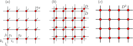
The tensor network ansatz describes quantum many-body states in an exponentially large Hilbert space in terms of local tensors $\mathbf{T}$ describing local degrees of freedom. A graphical representation of a tensor network state for a spin model on a square lattice is presented in Fig. 1(a), for which the wavefunction is written as

$$|\psi\rangle=\sum_{\{\sigma\}}{\mbox{tTr}\{\mathbf{T}^{[1],s_{1}}\mathbf{T}^{[2],s_{2}}\cdots\mathbf{T}^{[N],s_{N}}\}|s_{1},s_{2},\cdots,s_{N}\rangle},$$

where $\mathbf{T}^{[i],s_{i}}$ denotes the tensor of spin $s_{i}$ on site $i$ and $|\sigma\rangle\equiv|s_{1},s_{2},\cdots,s_{N}\rangle$ represents manybody spin configurations. The notation tTr is used to represent tensorial trace, generalization of the matrix trace to tensor networks where tensors are traced over the virtual modes.

Figure 1: (a) The tensor network wavefunction of a spin system on a square lattice, (b) The contraction of physical indices for calculating expectation values of a tensor network wavefunction, (c) this results in a tensor network of bond dimension $D^{2}$.

Figure 2: (a) First decompose each 4-index tensor (in open diamonds on dash lines) into two 3-index tensors (in black dots), then contract every 4 tensors in the shaded area into a 4-index tensor (in open square in (b)). (b) Repeat the decomposition-contraction procedure on a reduced and rotated lattice (in gray solid line). (c) The total effect is that each 2 $\times$ 2 cluster on a fine lattice (in dash lines) is coarse grained into a super site (in open diamond) on a coarse grained lattice; note that the lattice orientation can be restored after every two iterations.

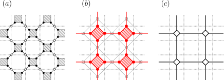
If one were to calculate an expectation value for a given observable given a PEPS state, it would require contraction of a double layer tensor network obtained by contracting over the physical bonds first as depicted on Fig. 1(b). This results in a tensor network with a squared bond dimension as shown on Fig. 1(c). The effort for contracting a tensor network either as Fig. 1(a) for single layer or as Fig. 1(c) for double layer grows exponentially with the system size. One way of exact contraction is to successively renormalize a $2\times 2$ block of sites into one super-site, as pointed out in Ref. ling-plq . Without approximation, the dimension of the virtual bond of a super-site in a double layer picture will grow as $D^{4n_{r}}$, where $n_{r}$ is the depth of the renormalization iteration (the linear size of the system is $L\sim 2^{n_{r}}$), thus approximate contraction becomes necessary. One of the ways to contract the tensor network approximately is the tensor renormalization method levinandnave , which was first proposed to contract a classical tensor network. Later on this method was generalized to deal with quantum systems gu-prb78-205116 ; jiang-prl101-090603 . The contraction method on a square lattice can be described in Fig. 2. First each 4-index $\mathbf{T}$-tensor is decomposed into two 3-index $\mathbf{S}$-tensors,

$$T^{\textrm{B}}_{ijkl}=\sum_{\alpha}S^{1}_{ij\alpha}{S^{3}}_{kl\alpha},$$ (2)

$$T^{\textrm{A}}_{jkli}=\sum_{\alpha}S^{2}_{jk\alpha}{S^{4}}_{li\alpha},$$ (3)

where $\mathbf{T}^{\textrm{ B,A}}$ denote two ways of tensor decomposition according to Eq.(2)(3) respectively. In the next step the four $\mathbf{S}$-tensors in the shaded area in Fig. 2(a) are contracted to form a coarse tensor on a reduced and rotated lattice,

$$T^{\prime}_{\alpha\beta\gamma\delta}=\sum_{ijkl}S^{2}_{jk\alpha}S^{3}_{kl\beta}S^{4}_{li\gamma}S^{1}_{ij\delta}.$$ (4)

This decomposition-contraction procedure can be applied once again on the rotated lattice (Fig. 2(b)) to obtain a coarse lattice of half the length (Fig 2(c)), and whose orientation of the lattice is equal to the original one.

A singular value decomposition (SVD) is then done to decompose a $\mathbf{T}$-tensor into two $\mathbf{S}$-tensors,

$$T^{\textrm{B}}_{ijkl}=\sum_{\alpha=1}^{D^{2}}U_{ij\alpha}\Lambda_{\alpha}V_{kl\alpha}.$$ (5)

To prevent an exponential increase of the computational cost, one only keeps the largest $D_{\textrm{cut}}$ (also referred to as $\chi$) singular values; this approximation maximizes the 2-norm of vectorized $\mathbf{T}$ for a fixed $D_{\textrm{cut}}$,

$$\widetilde{T}^{\textrm{B}}_{ijkl}\approx\sum_{\alpha=1}^{D_{\textrm{cut}}}\bar{U}_{ij\alpha}\bar{\Lambda}_{\alpha}\bar{V}_{kl\alpha},$$ (6)

where $\bar{\mathbf{M}}$ denotes taking the leading $D_{\textrm{cut}}$ columns of a matrix $\mathbf{M}$ (or leading singular values of a diagonal matrix). A common strategy is to absorb the diagonal matrix $\bar{\mathbf{\Lambda}}$ into isometries $\bar{\mathbf{U}}$ and $\bar{\mathbf{V}}$ to obtain the $\mathbf{S}$-tensors, $\mathbf{S}^{1}=\bar{\mathbf{U}}\sqrt{\bar{\mathbf{\Lambda}}}$ and $\mathbf{S}^{3}=\bar{\mathbf{V}}\sqrt{\bar{\mathbf{\Lambda}}}$, the same applies to $\mathbf{S}^{2},\mathbf{S}^{4}$.

II Variational Quantum Monte Carlo sampling and update

A variational quantum Monte Carlo (vQMC) method with tensor network states can now be based on the TERG contraction method to calculate the importance weight and the energy derivative. Following the notation of Ref. anders-prl99-220602 , we extract several key equations regarding measuring and updating. For a chosen configuration $|\sigma\rangle\equiv|s_{1},s_{2},\cdots,s_{N}\rangle$ we define a coefficient $W(\sigma)=\langle\sigma|\psi\rangle$, which is calculated by contracting a single layer tensor network as

$$W(\sigma)=\mbox{tTr}\{\mathbf{T}^{[1],s_{1}}\mathbf{T}^{[2],s_{2}}\cdots\mathbf{T}^{[N],s_{N}}\}.$$ (7)

The energy expectation value reads

$$\langle E\rangle=\frac{\sum_{\sigma}W^{2}(\sigma)E(\sigma)}{\sum_{\sigma}W^{2}(\sigma)},$$ (8)

where

$$E(\sigma)=\sum_{\sigma^{\prime}}\frac{W(\sigma^{\prime})}{W(\sigma)}\langle\sigma^{\prime}|H|\sigma\rangle.$$ (9)

The energy derivatives with respect to tensor elements $T^{\uparrow(\downarrow)}_{ijkl}$ are obtained via

$$\Big{<}\frac{\partial E}{\partial T^{\uparrow(\downarrow)}_{ijkl}}\Big{>}=2\langle\Delta^{\uparrow(\downarrow)}_{ijkl}(\sigma)E(\sigma)\rangle-2\langle\Delta^{\uparrow(\downarrow)}_{ijkl}(\sigma)\rangle\langle E(\sigma)\rangle,$$ (10)

the $\langle\rangle$ denotes Monte Carlo average and

$$\Delta^{\uparrow(\downarrow)}_{ijkl}=\frac{1}{W(\sigma)}\frac{\partial W(\sigma)}{\partial T^{\uparrow(\downarrow)}_{ijkl}}.$$ (11)

Let us define $\mathbf{B}(m)$ as the contraction of the tensor network for all sites except a site $m$:

$$\mathbf{B}(m)=\mbox{tTr}\{\cdots\mathbf{T}^{[m-1],s_{m-1}}\mathbf{T}^{[m+1],s_{m+1}}\cdots\},$$ (12)

in terms of which we can express the derivative of the weight (7) with respect to $T^{\uparrow(\downarrow)}_{ijkl}$ as

$$\frac{\partial W(\sigma)}{\partial T^{\uparrow(\downarrow)}_{ijkl}}=\sum_{m}B(m)_{ijkl}\delta_{s_{m},{\uparrow(\downarrow)}},$$ (13)

where we assume translation invariance symmetry, i.e. $\mathbf{T}^{[i],s}=\mathbf{T}^{[j],s}$ ($s=\uparrow,\downarrow$) for all sites $i,j$ in the lattice.

The program starts by randomly generating a spin configuration $|\sigma\rangle$ satisfying $\sum_{i}s_{i}=0$, i.e. we initialize our state to live in total spin 0 sector. Given $|\sigma\rangle$, one initializes and stores all the intermediate $\mathbf{T}^{\textrm{q},\textrm{p}}$-tensor at the site q of the $\textrm{p}^{\textrm{th}}$ coarse grained lattice. During the contraction, we also calculate and store scalars $f^{\textrm{q},\textrm{p}}\equiv\textrm{max}\{|{T}^{\textrm{q},\textrm{p}}_{ijkl}|\}$ for all $\mathbf{T}^{\textrm{q},\textrm{p}}$, then divide $T^{\textrm{q},\textrm{p}}_{ijkl}$ by $f^{\textrm{q},\textrm{p}}$ to avoid too large or too small singular values in the next iteration. If we define the tensor trace of the final contraction step as $g\equiv\mbox{tTr}\{\mathbf{T}^{[1],n_{r}}\mathbf{T}^{[2],n_{r}}\mathbf{T}^{[3],n_{r}}\mathbf{T}^{[4],n_{r}}\}$, where $n_{r}$ is the number of iterations of a tensor network contraction ($L=2^{\frac{n_{r}}{2}+1}$), then weight (7) can be written as

$$W(\sigma)=g\prod_{\textrm{q},\textrm{p}}f^{\textrm{q},\textrm{p}}.$$ (14)

Since we do not need to update the variational parameters $T^{\uparrow(\downarrow)}_{ijkl}$ in this work, we will discuss how to update a tensor network using energy derivatives with MC sampling technique elsewhere lingetal .

While describing the sampling procedure, we take the nearest neighbor Antiferromagnetic Heisenberg interaction as an example. Generalization to other Hamiltonian is straight forward. Starting from site 1 of the original tensor network, one looks for a pair of nearest neighbor spins that align anti-parallel with each other and flip them.

The trial configuration, which we denote as $|\sigma^{\prime}\rangle$, is accepted with probability

$$P=\mbox{min}\left[1,\frac{W^{2}(\sigma^{\prime})}{W^{2}(\sigma)}\right],$$ (15)

where the ratio is given by

$$\frac{W(\sigma^{\prime})}{W(\sigma)}=\frac{g^{\prime}}{g}\prod_{\textrm{q},\textrm{p}}\frac{f^{\prime\textrm{q},\textrm{p}}}{f^{\textrm{q},\textrm{p}}}.$$ (16)

To calculate the ratio (16), one needs to recompute some $\mathbf{T}^{\prime\textrm{q},\textrm{p}}$ tensors together with the corresponding scalars $f^{\prime\textrm{q},\textrm{p}}$ and $g^{\prime}$, store them in separate arrays for later updates. If a random number $r$ drawn from an uniform distribution on the interval $[0,1)$ satisfies $r<P$, the trial state $|\sigma^{\prime}\rangle$ is accepted, in which case $\mathbf{T}^{\textrm{q},\textrm{p}}$, $f^{\textrm{q},\textrm{p}}$ and $g$ are replaced by $\mathbf{T}^{\prime\textrm{q},\textrm{p}}$, $f^{\prime\textrm{q},\textrm{p}}$ and $g^{\prime}$, otherwise $|\sigma^{\prime}\rangle$ is rejected and the original configuration $|\sigma\rangle$ is kept. Moving through all the sites on the original lattice, one attempts to flip all encountered anti-parallel pairs, accepting or rejecting according to probability (15). This procedure is called a MC sweep. After each MC sweep, the energy and other observables of interest are measured. Flipping two neighboring spins does not require recomputing many $\mathbf{T}^{\prime\textrm{q},\textrm{p}}$ tensors, which makes the contraction fast. On the other hand, the update is local. To reduce the auto correlation length, one needs to complete a MC sweep before making a measurement, and the computational effort scales linearly with the system size $N=L^{2}$.

III The Antiferromagnetic Heisenberg model on square lattice

We use the simple update method of Xiang et al. jiang-prl101-090603 to obtain the converged wavefunction with various virtual bond dimension ($D=3,4,\cdots,20$). The simple update is an imaginary time evolution method to obtain the ground state wavefunction of an infinite lattice.

To implement the imaginary time evolution, we first make the Trotter decomposition of the partition function $e^{-\beta H}=[e^{-\tau\sum_{j}H_{j}}]^{\textrm{M}}$ for $\tau=\beta/{\textrm{M}}$, then we apply an evolution operator $e^{-\tau H_{j}}$ to the two nearest neighbor sites $\textrm{A},\textrm{B}$ as in Fig. 3(a). It is crucial to put the weight $\sqrt{\Lambda_{i}}$ to the open auxiliary modes to take into account the entanglement of the sub-system with the environment. The weights $\sqrt{\Lambda_{i}}$ are the singular values obtained in the previous evolution step on the corresponding bond. According to Ref. jiang-prl101-090603 an SVD is done to the joint tensor $\widetilde{\mathbf{T}}^{\textrm{A}}\widetilde{\mathbf{T}}^{\textrm{B}}$ to introduce a cut over the enlarged bond, and only the leading $D$ singular values and the corresponding left and right eigenvectors are kept as a projection to the sub-manifold of the Hilbert space where the wavefunction manifests. Here we made a crucial modification that drastically reduces the computational cost of decomposing the joint matrix $\widetilde{\mathbf{T}}^{\textrm{A}}\widetilde{\mathbf{T}}^{\textrm{B}}$ that is of size $d\textrm{D}^{3}\times d\textrm{D}^{3}$. As illustrated in Fig. 3(b), we first make QR(LQ) factorization of tensor $\widetilde{\mathbf{T}}^{\textrm{A(B)}}$ as $\widetilde{\mathbf{T}}^{\textrm{A}}=\mathbf{Q}^{\textrm{A}}\mathbf{R}^{\textrm{A}}$ and $\widetilde{\mathbf{T}}^{\textrm{B}}=\mathbf{L}^{\textrm{B}}\mathbf{Q}^{\textrm{B}}$, where $\mathbf{R}^{\textrm{A}}$ and $\mathbf{L}^{\textrm{B}}$ are right- and left-triangular matrices. Instead of a large tensor $\widetilde{\mathbf{T}}^{\textrm{A}}\widetilde{\mathbf{T}}^{\textrm{B}}$, the singular value decomposition is done on $\mathbf{R}^{\textrm{A}}\mathbf{L}^{\textrm{B}}$, which is essentially of size $d{\textrm{D}}\times d\textrm{D}$, as $\mathbf{R}^{\textrm{A}}\mathbf{L}^{\textrm{B}}=\mathbf{U\Lambda V}^{\textrm{T}}$. The leading computational cost is now the QR(LQ) decomposition that scales only to $D^{5}$. To obtain the evolved tensors on sites A and B, one has to remove the weight $\sqrt{\Lambda_{i}}$ from the decomposed tensors as described in Ref. jiang-prl101-090603 .

Figure 3: (a) A evolution operator is applied to the nearest neighbor sites A,B with weight $\sqrt{\Lambda_{i}}$ putting on the open bonds, (b) QR and LQ decompositions are done separately on $\widetilde{\mathbf{T}}^{\textrm{A}}$ and $\widetilde{\mathbf{T}}^{\textrm{B}}$ prior to the SVD step taken over the evolved bond between sites A,B. The computational cost is thus reduced from $D^{9}$ to $D^{5}$.

In the thermodynamic limit, the ground state of the Antiferromagnetic Heisenberg model spontaneously breaks the SU(2) symmetry, i.e. the magnetization is locked in one direction. To achieve a significant acceptance ratio for the Markov process with local spin flips, we intentionally break the SU(2) symmetry into the XY plane. To do this, we first attach a small ($h_{a}=0.001J$) staggered magnetic field in the $x$ direction to the isotropic Heisenberg Hamiltonian,

$$H=J\sum_{\langle i,j\rangle}{\bm{S}}_{i}\cdot{\bm{S}}_{j}+h_{a}\sum_{i}(-1)^{i_{x}+i_{y}}S_{i}^{x},\quad(J>0),$$ (17)

here $i_{x},i_{y}$ are $x,y$ coordinates of site $i$. We update the tensor network wavefunction using this modified Hamiltonian until it converges. Then we use the converged wavefunction to initialize a new update without the field. The Trotter steps of the imaginary time evolution is gradually reduced from $\tau=10^{-2}$ to $10^{-5}$. A convergence is reached when $\frac{\|\mathbf{T}^{\textrm{A(B)}}(\tau+100)-\mathbf{T}^{\textrm{A(B)}}(\tau)\|}{\|\mathbf{T}^{\textrm{A(B)}}(\tau)\|}<10^{-7}$, where $\mathbf{T}^{\textrm{A,B}}(\tau)$ is the vectorized tensor at time slice $\tau$, and is rescaled such that the largest magnitude of the tensor elements is 1. We then take these converged tensors of various bond dimension $D$ for the infinite lattice to compute expectation values of finite lattices with periodic boundary condition using MC sampling method.

One way to define the staggered magnetization is through the spin-spin correlation at the longest distance reger-prb37-5978

$$M^{2}=\sum_{\alpha}C^{\alpha}(L/2,L/2),$$ (18)

where $\alpha=x,y,z$, and

$$C^{\alpha}(L/2,L/2)=\frac{1}{L^{2}}\sum_{i}S^{\alpha}(i_{x},i_{y})S^{\alpha}(i_{x}+\frac{L}{2},i_{y}+\frac{L}{2}).$$

In Fig. 4, we present the staggered magnetization as a function of inverse virtual bond dimension $D$ for system sizes $L=4,8,16$. The solid lines represents the magnetization results for finite lattices obtained via SSE andersprb1997 and resonating valence bond (RVB) projection andersprb82-024407 methods. For a small size $L=4$, large bond dimension $D\geq 8$ gives the exact magnetization within the statistical error. For larger sizes $L=8,16$, the magnetization error at $D=16$ is 0.003(2) 0.013(2) respectively. Finite $D$ extrapolation gives the exact finite size magnetization for $L=8$, and reduces the magnetization error to 0.005(3) for $L=16$.

Figure 4: Staggered magnetization as a function of $1/D$ for $L=4,8,16$. The solid lines are finite size expectation value from SSE and RVB projection methods. The dashed lines are linear fits for all bond dimensions $D$ for sizes $L=8,16$ respectively.

Figure 5: Absolute error of the energy per bond as a function of the bond dimension $D$ for system sizes $L=4,8,16$ on a normal scale.

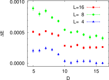
In Fig. 5 we present the absolute error of the finite size energy divided by the number of bonds as a function of virtual bond dimension $D$ for system sizes $L=4,8,16$. For all system sizes the energy error drops significantly at $D=10$ and at $D\in[10:16]$ plateaus seem to set in.

Figure 6: Spin-spin correlation $C^{\alpha}(L/2,L/2)$ ($\alpha=x,y,z$) as a function of $D$ for system sizes $L=4,8,16$. Solid lines are the $x,y$ components, dash lines show the $z$ component. Note that $C^{x}=C^{y}$ for the $U(1)$ symmetry.

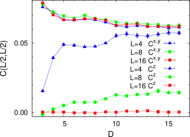
In Fig. 6 we show all three components of the spin-spin correlation at the longest distance $C^{\alpha}(L/2,L/2)$, $\alpha=x,y,z$. One can see that the $x,y$ components for different system sizes almost fall on top of each other. The $x,y$ components slightly drop at $D=5,10$ then followed by plateaus. The $z$ component, on the other hand, largely deviates from the $x$ and $y$ components. For $L=4$, the SU(2) symmetry is gradually restored with increasing bond dimension $D$; for $L=8$, there is a partial growth of $C^{z}(L/2,L/2)$ for increasing $D$; however for $L=16$, the $z$ component is zero for all available bond dimension $D$. Asymptotically, as $D$ increase, one could expect $C^{z}(L/2,L/2)$ grows to different values for different system sizes $L$, and for sufficiently large system size $C^{z}(L/2,L/2)\to 0$ due to automatic symmetry breaking.

Figure 7: Overlap of TPS $|\psi\rangle$ of various bond dimensions $D$ with the exact ground state wavefunction $|\psi\rangle_{0}$ obtained by exact diagonalization for system size $L=4$. For $D=16$ the overlap is 0.99979.

In Fig. 7 we calculate the overlap of the TPS wavefunction $|\psi\rangle$ for various bond dimensions $D$ with the exact ground state $|\psi\rangle_{0}$ obtained by an exact diagonalization for a $4\times 4$ system. For $D=16$ the overlap is 0.99979.

For all the data presented, the maximum number of singular values kept at each iteration step during the contraction is $D_{\textrm{cut}}=2D$ for all bond dimensions $D$.

IV Summary and discussion

In this paper, we proposed a variational Quantum Monte Carlo (vQMC) algorithm to evaluate a tensor network state of relative large bond dimensions. We illustrated the Monte Carlo (MC) sampling procedure in terms of the tensor entanglement renormalization group (TERG) contraction algorithm. We applied this method to the well studied Antiferromagnetic Heisenberg model on square lattice. Upon obtaining the ground state wavefunction via imaginary time evolution with essentially no notion of the lattice size, we evaluated the ground state energy and the staggered magnetization for systems on finite square lattices using MC sampling method. Not surprisingly, we found that the converged tensors obtained for the infinite lattice give very accurate results also when used for considered finite size lattices. The wavefunction of a finite bond dimension $D$ thus can be used to reliably extrapolate the expectation values in the thermodynamic limit through finite $D$ scaling followed by finite size scaling. We have shown that the tensor network ansatz based vQMC method is a promising way to go to a very large bond dimension and thus allowing reliable study of many interesting models.

We do not claim that the tensor product state (TPS) describing the ground state wavefunction for an infinite lattice obtained via the simple update is the ultimate solution for a finite lattice. One still need further optimization for a finite lattice if initializing from a TPS describing the infinite lattice. Many previous studies of 1 dimensional systems had used the matrix product state (MPS) obtained from an infinite chain algorithm itebd to initialize the optimization for a finite chain and obtained remarkably good results shi1d ; bogdan1d . We will discuss how to update tensors for a finite 2 dimensional system elsewhere lingetal . Another advantage of the MC sampling method is the possibility of incorporate lattice and spin symmetries into the MC sampling scheme to improve accuracy, which has been demonstrated in Ref. sandvik2dmps in the case of simulating 2 dimensional system via scale-renormalized MPSs. Since we obtained tensor directly from the simple update, we did not employ symmetries in the sampling procedure.