Finite motions from periodic frameworks with added symmetry

Abstract

Recent work from authors across disciplines has made substantial contributions to counting rules (Maxwell type theorems) which predict when an infinite periodic structure would be rigid or flexible while preserving the periodic pattern, as an engineering type framework, or equivalently, as an idealized molecular framework. Other work has shown that for finite frameworks, introducing symmetry modifies the previous general counts, and under some circumstances this symmetrized Maxwell type count can predict added finite flexibility in the structure.

In this paper we combine these approaches to present new Maxwell type counts for the columns and rows of a modified orbit matrix for structures that have both a periodic structure and additional symmetry within the periodic cells. In a number of cases, this count for the combined group of symmetry operations demonstrates there is added finite flexibility in what would have been rigid when realized without the symmetry. Given that many crystal structures have these added symmetries, and that their flexibility may be key to their physical and chemical properties, we present a summary of the results as a way to generate further developments of both a practical and theoretic interest.

Key Words: framework rigidity, periodic, symmetry, crystal systems, orbits

1 Introduction

The theory of periodic frameworks has undergone rapid and extensive development in the last four years (BorceaStreinuII; BorceaStreinuI; Theran; Ross). We now have necessary conditions (call them Maxwell counts) for such frameworks to be rigid, either with a fixed lattice of translations or with a flexible lattice of translations. Underlying much of the recent work are finite ‘lattice rigidity matrices’ for the equivalence classes of vertices and edges under the infinite group of translations $\mathbb{Z}^{d}$ in $d$-space. With the corresponding count of periodicity-preserving trivial motions under these constraints (typically $d$ translations), the number of rows, $e$, and columns, $dv+l$ (where $l$ is the number of lattice parameters) of these ‘orbit matrices’ lead to necessary Maxwell type counts for a framework to be infinitesimally rigid (BorceaStreinuI; Theran; Ross): $e\geq dv+l-d$.

The theory of finite symmetric frameworks has also experienced some breakout results, building on a decade or more of initial Maxwell type necessary conditions for frameworks of various symmetry groups (FGsymmax; FG4; cfgsw). In some key cases, these symmetry conditions predict finite motions for frameworks realized generically within the symmetry constraints, but whose graphs would be generically rigid without symmetry (KG1; bricard). Recently, key results of this work have been expressed in terms of ‘orbit rigidity matrices’ for the equivalence classes of vertices and edges under the group of symmetry operations ${\cal S}$ (BS4; BS6; BSWWorbit). With modified counts for the symmetry-preserving trivial motions $t_{\cal S}$, and with $e_{0}$ and $v_{0}$ denoting the number of edge orbits and vertex orbits under the group action of $\mathcal{S}$, respectively, these matrices lead to Maxwell type necessary counts for frameworks to be infinitesimally rigid: $e_{0}\geq dv_{0}-t_{\cal S}$.

Given that many crystal structures combine both periodic structure and symmetry within the unit cells, it is natural to investigate the interactions of these two types of group operations. So we will consider frameworks with ‘combined symmetry groups’ of the form $\mathbb{Z}^{d}\rtimes\cal S$, where $\mathbb{Z}^{d}$ is the group of translations of the framework, $\cal S$ is the group of additional symmetries of the framework, and $\rtimes$ denotes the semi-direct product of $\cal S$ acting on $\mathbb{Z}^{d}$. Note that every symmetry operation in such a group can be written as a unique product of an element of $\mathbb{Z}^{d}$ and an element of $\cal{S}$. However, since $\cal S$ is typically not normal in $\mathbb{Z}^{d}\rtimes\cal S$, the groups $\mathbb{Z}^{d}\rtimes\cal S$ are in general not direct products. Details on the semi-direct product can be found in any abstract algebra text, such as DummitFoote. In Section 6 we will introduce combined ‘orbit matrices’ for the groups $\mathbb{Z}^{d}\rtimes\cal S$. Combined with the counts of the trivial motions which preserve both symmetry and periodicity, this will provide extended Maxwell type necessary counts for infinitesimal rigidity. In this setting we:

1. count the rows of the combined orbit matrix: one row per orbit of edges $r=e_{0}$;

2. count the columns of the combined orbit matrix: one vector column per orbit of vertices plus columns for symmetry-preserving lattice deformations: $c=dv_{0}+\ell_{\cal S}$;

3. the dimension of the space of trivial motions (translations) left by symmetries: $t_{\cal S}$.

The minimum dimension of the space of non-trivial symmetry-preserving infinitesimal periodic motions of the periodic structure is:

$$m=c-t_{\cal S}\ \ -r\quad\text{or}\quad m=dv_{0}+\ell_{\cal S}-t_{\cal S}\ \ -e_{0}.$$

This is compared with the corresponding count on the graph without symmetry, where with orbits of size $k_{{\cal S}}$ and no fixed edges or vertices, for the fully flexible lattice, we would anticipate:

$$m=d(k_{{\cal S}}v_{0})+{d+1\choose 2}-d\ \ -(k_{{\cal S}}e_{0}).$$

In addition, if we choose the positions of the vertices generically within the symmetry (i.e., make one generic choice for each orbit of vertices) then the predicted infinitesimal motions will be finite flexes (asiroth; BS6; BSWWorbit).

The results are a surprise – adding symmetry can sometimes cause additional flexibility beyond what the original graph without symmetry would exhibit in the periodic lattice. These more flexible examples include symmetries such as inversive symmetry, or half-turn symmetry with a mirror, found in a number of crystals, such as zeolites. Recent studies have confirmed that flexibility is a feature of natural zeolites (Thorpe) and contributes to their physical and chemical properties. In turn, this suggests that predicted flexibility in a computer designed theoretical  ‘zeolite’ would be a criterion for selecting which theoretical compounds should be synthesized for further testing.

When adding symmetry to a periodic lattice structure, we must consider the flexibility that this symmetry allows in the lattice structure. Inversive symmetry will be a key example, as it fits all possible lattice deformations (it occurs in ‘triclinic lattices’), and the addition of this symmetry to the framework generates flexes from frameworks that previously were minimally rigid, while preserving the full range of possible flexes of the lattice itself.

In contrast, only certain types of lattices leave open the addition of a half-turn symmetry in $3$-space. A half-turn parallel to a side of the lattice requires that side to be perpendicular to the remaining parallelogram face. This leaves only four of the six possible flexes of the lattice (monoclinic lattices), but it does predict additional flexes. Similarly, mirrors of symmetry can fit parallel to faces of the lattice, and restrict the shapes to monoclinic lattices, with the variable angle now parallel to the mirror.

We can also have a larger symmetry group, with several generators. For example, monoclinic prismatic crystals, such as some forms of zeolite, have the symmetry group $\mathcal{C}_{2h}$ which has both a half-turn symmetry and a mirror. These restrict the possible lattice shapes to lattices with a parallelogram base (perpendicular to the axis, parallel to the mirror) and the vertical prism at right angles to the base. Other forms of zeolite have the added symmetry of $D_{2h}$, forcing the base to be a rectangle. Each symmetry group for the crystal structure and the associated crystal system requires some specific terms in the analysis, although patterns emerge, and we will present tables with rows for the combinations.

In the larger theory of rigidity of frameworks, infinitesimal flexes of ‘generic frameworks’ transfer to finite flexes, for appropriate versions of generic. This holds for generic frameworks without symmetry, for frameworks generic within the symmetry class, and for periodic frameworks. That property extends to these combined symmetry periodic frameworks, so we are talking about flexibility on a finite scale, at generic realizations for representatives of the orbits of the expanded group.

The outline of the paper is as follows. In §2, §3, and §4, we present the basic definitions and associated rigidity matrices for: (i) finite frameworks (§2); (ii) finite frameworks with symmetry and the orbit matrices (§3); and (iii) periodic frameworks with the associated lattice matrices (§4).

In §5, we introduce our method of inserting symmetry into the analysis of a periodic framework in dimensions $2$ and $3$. This includes a short summary of the wallpaper pattern types (dimension $2$) and crystal systems (dimension $3$) which arise as the possible lattices and restricted lattice variations for various symmetry groups in the corresponding dimension. §6 then presents some key examples in the plane for the groups $\mathbb{Z}^{2}\rtimes{\cal C}_{2}$ and $\mathbb{Z}^{2}\rtimes{\cal C}_{s}$ with various lattice flexibilities, as well as summary tables over all plane groups of the form $\mathbb{Z}^{2}\rtimes{\cal S}$. §7 presents key examples in $3$-space, with corresponding tables.

In §8 we briefly describe a range of extensions which are accessible using these methods, including: extensions to include fixed vertices and edges; extensions to additional plane and space groups; extensions to higher dimensions; and the companion static analysis of the frameworks.

The analysis is not complete. While we have covered groups of the form $\mathbb{Z}^{d}\rtimes{\cal S}$, some plane and space groups are not covered, namely those with 6-fold symmetry, or with glide reflections. As §8 illustrates, there is lots of room for additional exploration. We hope that this introduction, and the follow-up papers with detailed proofs for what is claimed here, will offer interested researchers tools to explore the range of examples of interest in their context.

2 Preliminaries on the rigidity of (finite) frameworks

A framework in $\mathbb{R}^{d}$ is a pair $(G,p)$, where $G$ is a finite simple (no loops or multiple edges) graph with vertex set $V(G)$ and edge set $E(G)$, and $p:V(G)\to\mathbb{R}^{d}$ is a map such that $p(i)\neq p(j)$ for all $\{i,j\}\in E(G)$. We also say that $(G,p)$ is a $d$-dimensional realization of the underlying graph $G$ (W1). For $i\in V(G)$, we say that $p_{i}:=p(i)$ is the joint of $(G,p)$ corresponding to $i$, and for $\{i,j\}\in E(G)$, we say that $p_{\{i,j\}}:=p(\{i,j\})$ is the bar of $(G,p)$ corresponding to $\{i,j\}$. Moreover, we let $v:=|V(G)|$ and $e:=|E(G)|$. It is often useful to identify $p$ with a vector in $\mathbb{R}^{dv}$ by using the order on $V(G)$. In this case we also refer to $p$ as a configuration of $v$ points in $\mathbb{R}^{d}$.

A framework $(G,p)$ in $\mathbb{R}^{d}$ is flexible if there exists a continuous path, called a finite flex or mechanism, $p(t):[0,1]\to\mathbb{R}^{dv}$ such that

• $p(0)=p$;

• $\|p(t)_{i}-p(t)_{j}\|=\|p_{i}-p_{j}\|$ for all $0\leq t\leq 1$ and all $\{i,j\}\in E(G)$;

• $\|p(t)_{k}-p(t)_{l}\|\neq\|p_{k}-p_{l}\|$ for all $0<t\leq 1$ and some pair $\{k,l\}$ of vertices of $G$.

Otherwise $(G,p)$ is said to be rigid. For some alternate equivalent definitions of a rigid and flexible framework see asiroth, for example.

An infinitesimal motion of a framework $(G,p)$ in $\mathbb{R}^{d}$ is a function $u:V(G)\to\mathbb{R}^{d}$ such that

$$(p_{i}-p_{j})\cdot(u_{i}-u_{j})=0\quad\textrm{ for all }\{i,j\}\in E(G)\textrm{,}$$ (1)

where $u_{i}$ denotes the vector $u(i)$ for each $i$.

An infinitesimal motion $u$ of $(G,p)$ is an infinitesimal rigid motion (or trivial infinitesimal motion) if there exists a skew-symmetric matrix $S$ (a rotation) and a vector $t$ (a translation) such that $u_{i}=Sp_{i}+t$ for all $i\in V(G)$. Otherwise $u$ is an infinitesimal flex (or non-trivial infinitesimal motion) of $(G,p)$.

$(G,p)$ is infinitesimally rigid if every infinitesimal motion of $(G,p)$ is an infinitesimal rigid motion. Otherwise $(G,p)$ is said to be infinitesimally flexible (W1).

While an infinitesimally rigid framework is always rigid, the converse does not hold in general. asiroth however, showed that for ‘generic’ configurations, infinitesimal rigidity and rigidity are in fact equivalent.

The rigidity matrix of $(G,p)$ (which in structural engineering is also known as the compatibility matrix of $(G,p)$ (KG2; cfgsw)) is the $e\times dv$ matrix

$$\mathbf{R}(G,p)=\bordermatrix{&&&&i&&&&j&&&\cr&&&&&&\vdots&&&&&\cr\{i,j\}&0&\ldots&0&(p_{i}-p_{j})&0&\ldots&0&(p_{j}-p_{i})&0&\ldots&0\cr&&&&&&\vdots&&&&&}\textrm{,}$$

that is, for each edge $\{i,j\}\in E(G)$, $\mathbf{R}(G,p)$ has the row with $(p_{i}-p_{j})_{1},\ldots,(p_{i}-p_{j})_{d}$ in the columns $d(i-1)+1,\ldots,di$, $(p_{j}-p_{i})_{1},\ldots,(p_{j}-p_{i})_{d}$ in the columns $d(j-1)+1,\ldots,dj$, and $0$ elsewhere (W1). See also Example 3.1.

Note that if we identify an infinitesimal motion $u$ of $(G,p)$ with a column vector in $\mathbb{R}^{dv}$ (by using the order on $V(G)$), then the equations in (1) can be written as $\mathbf{R}(G,p)u=0$. So, the kernel of the rigidity matrix $\mathbf{R}(G,p)$ is the space of all infinitesimal motions of $(G,p)$. It is well known that the infinitesimal rigid motions arising from $d$ translations and $\binom{d}{2}$ rotations of $\mathbb{R}^{d}$ form a basis of the space of infinitesimal rigid motions of $(G,p)$, provided that the points $p_{1},\ldots,p_{v}$ span an affine subspace of $\mathbb{R}^{d}$ of dimension at least $d-1$ (W1). Thus, for such a framework $(G,p)$, we have $\textrm{nullity }\big{(}\mathbf{R}(G,p)\big{)}\geq d+\binom{d}{2}=\binom{d+1}{2}$ and $(G,p)$ is infinitesimally rigid if and only if $\textrm{nullity }\big{(}\mathbf{R}(G,p)\big{)}=\binom{d+1}{2}$ or equivalently, $\textrm{rank }\big{(}\mathbf{R}(G,p)\big{)}=dv-\binom{d+1}{2}$.

In particular, it follows that we can sometimes detect infinitesimal flexes in frameworks - and, by the result of asiroth, even predict finite flexes in generic frameworks - by simply counting vertices and edges:

Theorem 2.1 (Maxwell’s rule)

Let $(G,p)$ be a $d$-dimensional framework whose joints span an affine subspace of $\mathbb{R}^{d}$ of dimension at least $d-1$. If

$$e<dv-\binom{d+1}{2}\textrm{,}$$ (2)

then $(G,p)$ has an infinitesimal flex.

If the joints of $(G,p)$ are in generic position, then there even exists a finite flex of $(G,p)$.

3 Symmetry in frameworks

3.1 Symmetric frameworks and motions

Given a finite simple graph $G$ with vertex set $V(G)=\{1,\ldots,n\}$, and a map $p:V(G)\to\mathbb{R}^{d}$, a symmetry operation of the framework $(G,p)$ in $\mathbb{R}^{d}$ is an isometry $s$ of $\mathbb{R}^{d}$ such that for some $\alpha_{s}\in\textrm{Aut}(G)$, we have

$$s(p_{i})=p_{\alpha_{s}(i)}\quad\textrm{for all }i\in V(G)\textrm{, }$$

where $\textrm{Aut}(G)$ denotes the automorphism group of the graph $G$ (Hall; BS2; BS1). The set of all symmetry operations of a framework $(G,p)$ forms a group under composition, called the point group of $(G,p)$ (bishop; Hall; BS2; BS1). Since translating a framework does not change its rigidity properties, we may assume wlog that the point group of a framework is always a symmetry group, i.e., a subgroup of the orthogonal group $O(\mathbb{R}^{d})$ (BS2; BS1).

Throughout this paper, we will highlight the Schoenflies notation for the symmetry operations and symmetry groups, as this is one of the standard notations in the literature (see bishop; cfgsw; FGsymmax; FG4; Hall; KG1; KG2; BS2; BS4; BS1, for example). In the later tables for crystallographic groups, we will show three notations in parallel, to ensure clearer communication with multiple audiences.

In the Schoenflies notation, the groups we will focus on in our examples and tables are denoted by $\mathcal{C}_{s}$, $\mathcal{C}_{n}$, $\mathcal{C}_{nv}$, $\mathcal{C}_{nh}$, $\mathcal{C}_{i}$, $\mathcal{D}_{n}$, and $\mathcal{D}_{nh}$. For dimension $2$ and $3$, $\mathcal{C}_{s}$ is a symmetry group consisting of the identity $Id$ and a single reflection $s$, and $\mathcal{C}_{n}$ is a cyclic group generated by an $n$-fold rotation $C_{n}$. The only other possible type of symmetry group in dimension $2$ is the group $\mathcal{C}_{nv}$ which is a dihedral group generated by a pair $\{C_{n},s\}$. In dimension $3$, $\mathcal{C}_{nv}$ denotes any symmetry group that is generated by a rotation $C_{n}$ and a reflection $s$ whose corresponding mirror contains the rotational axis of $C_{n}$, whereas a symmetry group $\mathcal{C}_{nh}$ is generated by a rotation $C_{n}$ and the reflection $s$ whose corresponding mirror is perpendicular to the $C_{n}$-axis. The group $\mathcal{C}_{i}$ consists of the identity $Id$ and an inversion $i$ in $3$-space. Finally, $\mathcal{D}_{n}$ is generated by an $n$-fold rotation $C_{n}$ and a $2$-fold rotation $C_{2}$ whose rotational axes are perpendicular to each other, and $\mathcal{D}_{nh}$ is generated by the generators $C_{n}$ and $C_{2}$ of a group $\mathcal{D}_{n}$ and by a reflection $s$ whose mirror is perpendicular to the $C_{n}$-axis.

Given a symmetry group $\mathcal{S}$ in dimension $d$ and a graph $G$, we let $\mathscr{R}_{(G,\mathcal{S})}$ denote the set of all $d$-dimensional realizations of $G$ whose point group is either equal to $\mathcal{S}$ or contains $\mathcal{S}$ as a subgroup (BS2; BS1). In other words, the set $\mathscr{R}_{(G,\mathcal{S})}$ consists of all frameworks $(G,p)$ for which there exists a map $\phi:\mathcal{S}\to\textrm{Aut}(G)$ so that

$$s\big{(}p_{i}\big{)}=p_{\Phi(s)(i)}\textrm{ for all }i\in V(G)\textrm{ and all }s\in\mathcal{S}\textrm{.}$$ (3)

If a framework $(G,p)\in\mathscr{R}_{(G,\mathcal{S})}$ satisfies the equations in (3) for the map $\Phi:\mathcal{S}\to\textrm{Aut}(G)$, we say that $(G,p)$ is of type $\Phi$. It is shown in BS4; BS1 that if the map $p$ of a framework $(G,p)\in\mathscr{R}_{(G,\mathcal{S})}$ is injective, then $(G,p)$ is of a unique type $\Phi$ and $\Phi$ is necessarily also a homomorphism. For simplicity, we therefore assume that the map $p$ of any framework $(G,p)$ considered in this paper is injective (i.e., $p_{i}\neq p_{j}$ if $i\neq j$). In particular, this allows us (with a slight abuse of notation) to use the terms $p_{s(i)}$ and $p_{\Phi(s)(i)}$ interchangeably, where $i\in V(G)$ and $s\in\mathcal{S}$. In general, if the type $\Phi$ is clear from the context, we often simply write $s(i)$ instead of $\Phi(s)(i)$.

An infinitesimal motion $u$ of a framework $(G,p)\in\mathscr{R}_{(G,\mathcal{S})}$ is $\mathcal{S}$-symmetric if

$$s\big{(}u_{i}\big{)}=u_{s(i)}\textrm{ for all }i\in V(G)\textrm{ and all }s\in\mathcal{S}\textrm{,}$$ (4)

i.e., if $u$ is unchanged under all symmetry operations in $\mathcal{S}$ (see also Figure 1(a) and (b)).

Figure 1: Infinitesimal motions of frameworks in the plane: (a) a $\mathcal{C}_{s}$-symmetric infinitesimal flex; (b) a $\mathcal{C}_{s}$-symmetric infinitesimal rigid motion; (c) an infinitesimal flex which is not $\mathcal{C}_{s}$-symmetric.

Note that if for $(G,p)\in\mathscr{R}_{(G,\mathcal{S})}$, we choose a set of representatives $\{1,\ldots,v_{0}\}$ for the orbits $\mathcal{S}(i)=\{s(i)|\,s\in\mathcal{S}\}$ of vertices of $G$ under the group action of $\mathcal{S}$, then the positions of all joints of $(G,p)$ are uniquely determined by the positions of the joints $p_{1},\ldots,p_{v_{0}}$ and the symmetry constraints imposed by $\mathcal{S}$. Similarly, an $\mathcal{S}$-symmetric infinitesimal motion $u$ of $(G,p)$ is uniquely determined by the velocity vectors $u_{1},\ldots,u_{v_{0}}$ for the representative vertices.

The following extension of the theorem of asiroth shows that an analysis of the ‘$\mathcal{S}$-symmetric’ infinitesimal rigidity properties of a symmetric framework can be used to also detect finite flexes in the framework, provided that its joints are positioned generically within the symmetry.

Theorem 3.1

(BS6) (see also BS4) Let $\mathcal{S}$ be a symmetry group in dimension $d$, and let $(G,p)\in\mathscr{R}_{(G,\mathcal{S})}$ be a framework whose joints span all of $\mathbb{R}^{d}$, in an affine sense. If $(G,p)$ is generic modulo the symmetry group $\mathcal{S}$, i.e., the vertices of a set of representatives for the vertex orbits under the action of $\mathcal{S}$ are placed in ‘generic’ positions (see BS6; BS1; BSWWorbit for details), and $(G,p)$ also possesses an $\mathcal{S}$-symmetric infinitesimal flex, then $(G,p)$ also has a finite flex which preserves all the symmetries in $\mathcal{S}$ throughout the path.

3.2 Orbit rigidity matrices for symmetric frameworks

To determine whether a given framework $(G,p)\in\mathscr{R}_{(G,\mathcal{S})}$ possesses an $\mathcal{S}$-symmetric infinitesimal flex, we can use the techniques from group representation theory described in FGsymmax; KG2; BS6; BS2. In the recent paper BSWWorbit the ‘orbit matrix’ was introduced as a simplifying alternative to detect symmetric infinitesimal motions in symmetric frameworks and to predict finite flexes for configurations which are generic within the symmetry. In fact, it is shown in BSWWorbit that the orbit matrix is equivalent to the submatrix block $\widetilde{\mathbf{R}}_{1}(G,p)$ studied in BS6, but the construction is transparent, and the entries in the matrix can be explicitly derived, without using techniques from group representation theory.

For a $d$-dimensional framework $(G,p)\in\mathscr{R}_{(G,\mathcal{S})}$ which has no joint that is ‘fixed’ by a non-trivial symmetry operation in $\mathcal{S}$ (i.e., $(G,p)$ has no joint $p_{i}$ with $s(p_{i})=p_{i}$ for some $s\in\mathcal{S}$, $s\neq id$), the construction of the orbit matrix becomes particularly easy (see Definition 3.1), because, in this case, the orbit matrix has a set of $d$ columns for each orbit of vertices under the group action of $\mathcal{S}$.

Definition 3.1

(BSWWorbit) Let $\mathcal{S}$ be a symmetry group in dimension $d$ and let $(G,p)\in\mathscr{R}_{(G,\mathcal{S})}$ be a framework which has no joint that is ‘fixed’ by a non-trivial symmetry operation in $\mathcal{S}$. Further, let $\mathscr{O}_{V(G)}=\{1,\ldots,v_{0}\}$ be a set of representatives for the orbits $\mathcal{S}(i)=\{s(i)|\,s\in\mathcal{S}\}$ of vertices of $G$. For each edge orbit $\mathcal{S}(e)=\{s(e)|\,s\in\mathcal{S}\}$ of $G$, the orbit matrix $\mathbf{O}(G,p,\mathcal{S})$ of $(G,p)$ has the following corresponding ($dv_{0}$-dimensional) row vector:

Case 1:

If the two end-vertices of the edge $e$ lie in distinct vertex orbits, then there exists an edge in $\mathcal{S}(e)$ that is of the form $\{a,s(b)\}$ for some $s\in\mathcal{S}$, where $a,b\in\mathscr{O}_{V(G)}$. The row we write in $\mathbf{O}(G,p,\mathcal{S})$ is:

$$\bordermatrix{&&a&&b&\cr&0\ldots 0&\big{(}p_{a}-s(p_{b})\big{)}&0\ldots 0&\big{(}p_{b}-s^{-1}(p_{a})\big{)}&0\ldots 0}\textrm{.}$$

Case 2:

If the two end-vertices of the edge $e$ lie in the same vertex orbit, then there exists an edge in $\mathcal{S}(e)$ that is of the form $\{a,s(a)\}$ for some $s\in\mathcal{S}$, where $a\in\mathscr{O}_{V(G)}$. The row we write in $\mathbf{O}(G,p,\mathcal{S})$ is:

$$\bordermatrix{&&a&\cr&0\ldots 0&\big{(}2p_{a}-s(p_{a})-s^{-1}(p_{a})\big{)}&0\ldots 0}\textrm{.}$$

Example 3.2.1 To illustrate the above definition, we consider the $2$-dimensional framework $(G,p)$ with point group $\mathcal{C}_{2}=\{id,C_{2}\}$ depicted in Figure 2 as an example. If we denote $p_{1}=(a,b)$, $p_{2}=(c,d)$, $p_{3}=(-a,-b)$, and $p_{4}=(-c,-d)$, then the rigidity matrix of $(G,p)$ is

$$\bordermatrix{&1&2&{3}=C_{2}(1)&{4}=C_{2}(2)\cr\{1,2\}&(a-c,b-d)&(c-a,d-b)&0\ 0&0\ 0\cr\{1,C_{2}(2)\}&(a+c,b+d)&0\ 0&0\ 0&(-a-c,-b-d)\cr C_{2}(\{1,2\})&0\ 0&0\ 0&(c-a,d-b)&(a-c,b-d)\cr C_{2}(\{1,C_{2}(2)\})&0\ 0&(a+c,b+d)&(-a-c,-b-d)&0\ 0}$$

The orbit matrix $\mathbf{O}(G,p,\mathcal{C}_{2})$ of $(G,p)$ will only have two rows, one for each representative of the edge orbits under the action of $\mathcal{C}_{2}$. (Note that if we are only interested in infinitesimal motions and self-stresses of $(G,p)$ that are $\mathcal{C}_{2}$-symmetric, then it indeed suffices to focus on the first two rows of the rigidity matrix of $(G,p)$. The other two rows are clearly redundant in this symmetric context!). Further, $\mathbf{O}(G,p,\mathcal{C}_{2})$ will have only four columns, because $G$ has only two vertex orbits under the action of $\mathcal{C}_{2}$, represented by the vertices $1$ and $2$, for example, and each of the joints $p_{1}$ and $p_{2}$ has two degrees of freedom in the plane. Since both edge orbits satisfy Case 2 in Definition 3.1, $\mathbf{O}(G,p,\mathcal{C}_{2})$ has the following form:

$$\bordermatrix{&1&2\cr\{1,2\}&(p_{1}-p_{2})&(p_{2}-p_{1})\cr\{1,C_{2}(2)\}&\big{(}p_{1}-C_{2}(p_{2})\big{)}&\big{(}p_{2}-C_{2}^{-1}(p_{1})\big{)}\cr}=\bordermatrix{&1&2\cr&(a-c,b-d)&(c-a,d-b)\cr&(a+c,b+d)&(c+a,d+b)\cr}$$

$\square$

Figure 2: The framework $(G,p)\in\mathscr{R}_{(G,\mathcal{C}_{2})}$ (a) and its corresponding symmetric orbit graph (b).

We can use the ‘symmetric orbit graph’ to describe the underlying combinatorial structure for the orbit matrix of a symmetric framework (see also Figure 2 (b)):

Definition 3.2

The symmetric orbit graph $G_{\mathcal{S}}$ of a framework $(G,p)\in\mathscr{R}_{(G,\mathcal{S})}$ is a labeled multigraph (it may contain loops and multiple edges) whose vertex set $\{1,\ldots,v_{0}\}$ is a set of representatives of the vertex orbits of $G$ under the action of $\mathcal{S}$, and whose edge set is defined as follows. For each edge orbit of $G$ under the action of $\mathcal{S}$, there exists one edge in $G_{\mathcal{S}}$: for an edge orbit satisfying Case 1 of Definition 3.1, $G_{\mathcal{S}}$ has a directed edge connecting the vertices $a$ and $b$. If the edge is directed from $a$ to $b$, it is labeled with $s$, and if the edge is directed from $b$ to $a$, it is labeled with $s^{-1}$. For simplicity we omit the label and the direction of the edge if $s=id$. Similarly, for an edge orbit satisfying Case 2 of Definition 3.1, $G_{\mathcal{S}}$ has a loop at the vertex $a$ which is labeled with $s$.

The key result for the orbit matrix is the following:

Theorem 3.2

(BSWWorbit) Let $S$ be a symmetry group and let $(G,p)$ be a framework in $\mathscr{R}_{(G,\mathcal{S})}$. Then the solutions to $\mathbf{O}(G,p,\mathcal{S})u=0$ are isomorphic to the space of $\mathcal{S}$-symmetric infinitesimal motions of the original framework $(G,p)$.

As an immediate consequence of Theorems 3.1 and 3.2, we have the following Maxwell type counting rule for detecting finite ‘symmetry-preserving’ flexes in symmetric frameworks:

Theorem 3.3

(BS4; BS6; BSWWorbit) Let $\mathcal{S}$ be a symmetry group in dimension $d$ and let $(G,p)$ be a framework in $\mathscr{R}_{(G,\mathcal{S})}$ which has no joint that is ‘fixed’ by a non-trivial symmetry operation in $S$. Further, let $e_{0}$ and $v_{0}$ denote the number of edge orbits and vertex orbits under the action of $\mathcal{S}$, respectively, and let $triv_{\mathcal{S}}$ denote the dimension of the space of $\mathcal{S}$-symmetric infinitesimal rigid motions of $(G,p)$. If

$$e_{0}<dv_{0}-triv_{\mathcal{S}}\textrm{,}$$ (5)

then $(G,p)$ has an $\mathcal{S}$-symmetric infinitesimal flex. If the joints of $(G,p)$ also span all of $\mathbb{R}^{d}$ (in an affine sense) and are in generic position modulo $\mathcal{S}$, then there even exists a finite flex of $(G,p)$ which preserves the symmetries in $\mathcal{S}$ throughout the path.

The dimension $triv_{\mathcal{S}}$ of the space of $\mathcal{S}$-symmetric infinitesimal rigid motions of $(G,p)\in\mathscr{R}_{(G,\mathcal{S})}$ can easily be computed using the techniques described in BS4; BS2. In particular, in dimension 2 and 3, $triv_{\mathcal{S}}$ can be deduced immediately from the character tables given in cfgsw. Thus, in order to check condition (5), it is only left to determine the size of the orbit matrix $\mathbf{O}(G,p,\mathcal{S})$, which in turn requires only a simple count of the vertex orbits and edge orbits of the graph $G$ under the action of $\mathcal{S}$ (see also Example 3.2.1 and Table 1).

Note that for a symmetry group $\mathcal{S}$ in any dimension $d$, the dimension $t_{\mathcal{S}}$ of the space of $S$-symmetric infinitesimal translations can also be obtained in a very intuitive way, without using the techniques in BS4; BS2: if for a symmetry operation $s\in\mathcal{S}$, we let $F_{s}$ denote the symmetry element corresponding to $s$ (i.e., $F_{s}=\{a\in\mathbb{R}^{d}\,|s(a)=a\}$), then $t_{\mathcal{S}}$ is simply the dimension of the symmetry element of the group $\mathcal{S}$, i.e., the dimension of the linear subspace $\bigcap_{s\in\mathcal{S}}F_{s}$ of $\mathbb{R}^{d}$, because the initial velocity vectors of an $\mathcal{S}$-symmetric infinitesimal translation must all be contained in the space $\bigcap_{s\in\mathcal{S}}F_{s}$.

For example, for the ‘reflectional’ symmetry group $\mathcal{C}_{s}=\{id,\sigma\}$ in dimension $d$, it is easy to see that the space of $\mathcal{C}_{s}$-symmetric infinitesimal translations is of dimension $(d-1)$, since it consists of those translations whose velocity vectors are elements of the $(d-1)$-dimensional mirror-plane $F_{\sigma}=\mathbb{R}^{d}\cap F_{\sigma}=F_{id}\cap F_{\sigma}=\bigcap_{s\in\mathcal{C}_{s}}F_{s}$ corresponding to $\sigma$ (see also Figure 1 (b)).

However, finding the dimension of the space of $\mathcal{S}$-symmetric infinitesimal rotations heuristically, without the techniques in BS4; BS2, becomes increasingly hard, if not impossible, in dimensions $>3$.

Example 3.2.2 Let’s apply Theorem 3.3 to the framework $(G,p)$ we considered in Example 3.2.1 (see also Figures 2 (a) and 3). We clearly have $dv_{0}=2\cdot 2=4$ and $e_{0}=2$. Further, we have $triv_{\mathcal{C}_{2}}=1$, since the only infinitesimal rigid motions that are $\mathcal{C}_{2}$-symmetric are the ones that correspond to rotations about the origin (see BS4; BS2 for details). Thus, we have

$$e_{0}=2<3=dv_{0}-triv_{\mathcal{C}_{2}}\textrm{.}$$

So, by Theorem 3.3, we may conclude that any realization of $G$ which is ‘generic’ modulo the half-turn symmetry has a symmetry-preserving finite flex (Figure 3). $\square$

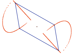
Figure 3: A $\mathcal{C}_{2}$-symmetric infinitesimal flex of the framework from Example 3.2.1 (a) and the path taken by the joints of the framework under the corresponding symmetry-preserving finite flex (b).

Note that the standard (non-symmetric) Maxwell count also detects a finite flex for the framework in Example 3.2, since for the graph $G$, we have $e=4<5=2v-3$. However, as shown in BSWWorbit, there exist a range of interesting and famous examples in $3$-space, including the Bricard octahedra (bricard; Stachel) and the flexible cross-polytopes (Stachel4D), which can be shown to be flexible via the symmetric count in Theorem 3.3, but not with the standard non-symmetric Maxwell-Laman type counts for rigidity.

The following table shows the symmetric Maxwell type counts for a selection of point groups $\mathcal{S}$ in $3$-space. For simplicity at this stage, we assume that no joint and no bar is fixed by a non-trivial element in $\mathcal{S}$, so that all vertex orbits and edge orbits under the action of $\mathcal{S}$ have the same size $k_{\mathcal{S}}$. (Recall that a joint $p_{i}$ is fixed by $s\in\cal S$ if $s(p_{i})=p_{i}$; a bar $\{p_{i},p_{j}\}$ is fixed by $s\in\cal S$ if either $s(p_{i})=p_{i}$ and $s(p_{j})=p_{j}$ or $s(p_{i})=p_{j}$ and $s(p_{j})=p_{i}$). So, in particular, both the number of joints, $v$, and the number of bars, $e$ are divisible by $k_{\mathcal{S}}$. A necessary condition for rigidity in $3$-space is $e\geq 3v-6$ (recall Theorem 2.1). For each group $\mathcal{S}$ in Table 1, $e$ is chosen to be the smallest number which satisfies $e\geq 3v-6$ and is divisible by $k_{\mathcal{S}}$; that is, $e$ is chosen to be the least number of edges for the framework to be rigid without symmetry and to be compatible with the symmetry constraints given by $\mathcal{S}$. The integer $f_{\mathcal{S}}$ in the final column indicates an $f_{\mathcal{S}}$-dimensional space of $\mathcal{S}$-symmetric infinitesimal flexes if $f_{\mathcal{S}}>0$, and a $(-f_{\mathcal{S}})$-dimensional space of $\mathcal{S}$-symmetric self-stresses if $f_{\mathcal{S}}<0$. (See Section LABEL:subsec:Stresses for more on self-stresses.)

Table 1: Impact of some $3$-space point groups on counts for rigidity.

$$\begin{array}[]{|c|c|c|c|c|c|c|}\hline\cr\text{{\color[rgb]{.5,.5,.5}$\mathcal{S}$}}&{\color[rgb]{.5,.5,.5}k_{\cal S}}&{\color[rgb]{.5,.5,.5}triv_{{\cal S}}}&{\color[rgb]{.5,.5,.5}e}&\text{{\color[rgb]{.5,.5,.5}$e_{0}$ }}&\text{{\color[rgb]{.5,.5,.5}$3v_{0}-triv_{{\cal S}}$}}&\text{{\color[rgb]{.5,.5,.5}$f_{\mathcal{S}}$}}\\ \hline\cr\mathcal{C}_{1}&1&6&3v-6&3v_{0}-6&3v_{0}-6&0\\ \hline\cr\mathcal{C}_{i}&2&3&3v-6&3v_{0}-3&3v_{0}-3&0\\ \hline\cr\mathcal{C}_{2}&2&2&3v-6&3v_{0}-3&3v_{0}-2&1\\ \hline\cr\mathcal{C}_{s}&2&3&3v-6&3v_{0}-3&3v_{0}-3&0\\ \hline\cr\mathcal{C}_{2h}&4&1&3v-4&3v_{0}-1&3v_{0}-1&0\\ \hline\cr\mathcal{D}_{2h}&8&0&3v&3v_{0}&3v_{0}-0&0\\ \hline\cr\mathcal{C}_{4}&4&2&3v-4&3v_{0}-1&3v_{0}-2&(-1)\\ \hline\cr\mathcal{C}_{3}&3&2&3v-6&3v_{0}-2&3v_{0}-2&0\\ \hline\cr\end{array}$$

The final column of Table 1 indicates that at ‘generic’ configurations, the frameworks with $\mathcal{C}_{2}$ symmetry always have a finite flex, while those with $\mathcal{C}_{4}$ symmetry are always stressed.

4 Periodic frameworks

4.1 From infinite periodic frameworks to a finite orbit graph

Let $\widetilde{G}$ be a simple infinite graph with finite degree at each vertex. Let $\widetilde{p}$ be a placement of the vertices $V(\widetilde{G})$ in $\mathbb{R}^{3}$, such that the resulting framework $(\widetilde{G},\widetilde{p})$ is invariant with respect to three linearly independent translations ${\bf t}_{1},{\bf t}_{2},{\bf t}_{3}\in\mathbb{R}^{3}$. We assume without loss of generality that ${\bf t}_{1}$ lies on the $x$-axis, and ${\bf t}_{2}$ lies in the $xy$-plane. Let $L$ be the matrix whose rows are these translations:

$$L=\left[\begin{array}[]{c}{\bf t}_{1}\\ {\bf t}_{2}\\ {\bf t}_{3}\end{array}\right]=\left[\begin{array}[]{ccc}t_{11}&0&0\\ t_{21}&t_{22}&0\\ t_{31}&t_{32}&t_{33}\end{array}\right].$$

We call the pair $(\langle\widetilde{G},L\rangle,\widetilde{p})$ a periodic framework. This definition can be adapted to describe periodic objects in $d$ dimensions, but here our focus will be on crystal-like structures in two and three dimensions. In two dimensions,

$$L=\left[\begin{array}[]{c}{\bf t}_{1}\\ {\bf t}_{2}\end{array}\right]=\left[\begin{array}[]{cc}t_{11}&0\\ t_{21}&t_{22}\end{array}\right],$$

and the other definitions are similarly adapted.

The three translations ${\bf t}_{1},{\bf t}_{2},{\bf t}_{3}$ define a parallelepiped called the unit cell. This can be equivalently described by three lengths $a,b,c$, and three angles $\alpha,\beta,\gamma$, as illustrated in Figure 4. These coordinates are standard in crystallography texts (Wiki). We may obtain one representation from the other by a change of coordinates.

Figure 4: The unit cell defined by the translations ${\bf t}_{1},{\bf t}_{2},{\bf t}_{3}$. The unit cube (all side lengths $1$) is shown in the dashed lines.

A copy of the unit cell centered at the origin is given by

$$U=\left\{a_{1}{\bf t}_{1}+a_{2}{\bf t}_{2}+a_{3}{\bf t}_{3}\ |\ -\frac{1}{2}\leq a_{i}<\frac{1}{2}\right\},$$

with its boundary defined to be the boundary of the closed parallelepiped:

$$\overline{U}=\left\{a_{1}{\bf t}_{1}+a_{2}{\bf t}_{2}+a_{3}{\bf t}_{3}\ |\ |a_{i}|\leq\frac{1}{2}\right\}.$$

We assume without loss of generality that no vertex of $V(\widetilde{G})$ lies on the boundary of the unit cell (we may simply translate the framework $(\langle\widetilde{G},L\rangle,\widetilde{p})$ until no vertex lies on the boundary).

The translations ${\bf t}_{1},{\bf t}_{2},{\bf t}_{3}$ generate a crystalline lattice ${\bf t}_{1}\mathbb{Z}\times{\bf t}_{2}\mathbb{Z}\times{\bf t}_{3}\mathbb{Z}$. This lattice partitions $\mathbb{R}^{3}$ into copies of the unit cell, each containing exactly one lattice point. Let each cell be centered at that lattice point, and let the cells be indexed by $\mathbb{Z}^{3}$ according to the lattice point they contain.

We now use this partition to define a finite labeled graph $G$ which represents the periodic framework, and can be used to study its rigidity. The edges of this graph are labeled invertibly by elements of the group $\mathbb{Z}^{3}$ in a way that captures the periodic structure of $(\langle\widetilde{G},L\rangle,\widetilde{p})$. Figure 5 illustrates this process for the analogous 2-dimensional case, in which edges are labeled by elements of the group $\mathbb{Z}^{2}$.

(a) $(\langle\widetilde{G},L\rangle,\widetilde{p})$

(b) $\langle G,n\rangle$

Figure 5: A 2-dimensional periodic framework (a) with the $(0,0)$-cell indicated. The periodic orbit graph is shown in (b).

Definition 4.1

The periodic orbit graph $\langle G,n\rangle$ of a periodic framework $(\langle\widetilde{G},L\rangle,\widetilde{p})$ is a labeled multigraph whose vertex set $V(G)=\{1,\ldots,v\}$ consists of the vertices appearing in the $(0,0,0)$-cell of $(\langle\widetilde{G},L\rangle,\widetilde{p})$. The edge set $E(G)$ and the labelling $n:E(G)\rightarrow\mathbb{Z}^{3}$ on these edges are defined as follows:

Case 1:

An edge $\widetilde{e}\in E(\widetilde{G})$ whose length is completely contained within the $(0,0,0)$-cell must connect two distinct vertices of $V(\widetilde{G})$ which also lie in the $(0,0,0)$-cell. For every such edge $\widetilde{e}$, define $e\in E(G)$ to be the edge connecting the corresponding vertices of $V(G)$. Assign this edge an arbitrary direction, and label it with $(0,0,0)$. For visual simplicity in our diagrams, edges labeled by the zero (identity) element appear as unlabeled, undirected edges.

Case 2:

Let $\widetilde{e}\in E(\widetilde{G})$ be an edge that crosses the boundary of the $(0,0,0)$-cell. In particular, suppose $\widetilde{e}$ connects the vertex $v$ in the $(0,0,0)$-cell with the vertex $w$ in the $(n_{1},n_{2},n_{3})$-cell. Then define $e\in E(G)$ to be a directed edge of $G$ that originates in the vertex $v$, terminates at the vertex $w$. Assign this directed edge the label $(n_{1},n_{2},n_{3})\in\mathbb{Z}^{3}$.

The periodic orbit graph $\langle G,n\rangle$ contains a set of representatives of the vertex and edge orbits of $(\langle\widetilde{G},L\rangle,\widetilde{p})$ under the action of $\mathbb{Z}^{3}$. Let ${p}$ be the restriction of $\widetilde{p}$ to the vertices of the $(0,0,0)$-cell, ${p}:V\rightarrow U.$ We call the pair $(\langle G,n\rangle,{p})$ the periodic orbit framework of $(\langle\widetilde{G},L\rangle,\widetilde{p})$, and the labeled multigraph $\langle G,n\rangle$ will be called the periodic orbit graph.

Let the edges $E(G)$ be ordered. An edge $e_{k}$ of $\langle G,n\rangle$ is denoted by $\{i,j;n_{k}\}$, where $i,j\in V(G)$ and $n_{k}\in\mathbb{Z}^{3}$. This edge corresponds to an equivalence class of bars in the periodic framework $(\langle\widetilde{G},L\rangle,\widetilde{p})$, which contains the bar $({p}_{i},{p}_{j}+n_{k}T)$, and all of its translates by $\sum a_{i}{\bf t}_{i}$, for integers $a_{i}$. This edge can be equivalently represented by $\{j,i;-n_{k}\}.$

It has been shown (Theran; Ross) that every ($d$-dimensional) periodic graph admits such a representation, and is invariant under the choice of unit cell of a specified size. It is also known that every finite directed multigraph whose edges are labeled with elements of the group $\mathbb{Z}^{d}$ can be realized as a $d$-dimensional periodic graph (Ross). In general, directed multigraphs whose edges are labeled by elements of a group, with the reverse direction implicitly labeled by the inverse group element, are known as gain graphs (GrossTucker).

4.2 Periodic rigidity and infinitesimal rigidity

We may define notions of rigidity and infinitesimal rigidity for the periodic framework $(\langle\widetilde{G},L\rangle,\widetilde{p})$ simply by a direct application of the ideas from Section 2. However, in this paper we are interested exclusively in motions and infinitesimal motions of $(\langle\widetilde{G},L\rangle,\widetilde{p})$ which preserve the periodicity of the framework. We say that $(\langle\widetilde{G},L\rangle,\widetilde{p})$ is periodic (infinitesimally) rigid if the only periodic (infinitesimal) motions of $(\langle\widetilde{G},L\rangle,\widetilde{p})$ are trivial. By defining rigidity and infinitesimal rigidity for a periodic orbit framework $(\langle G,n\rangle,{p})$, we are able to identify precisely these characteristics of the corresponding periodic framework, $(\langle\widetilde{G},L\rangle,\widetilde{p})$. Further details can be found in BorceaStreinuI; Theran; Ross.

Let $(\langle G,n\rangle,{p})$ be a periodic orbit framework, and let $e_{k}=\{i,j;n_{k}\}$ be an edge of $\langle G,n\rangle$, with $n_{k}=(n_{k1},n_{k2},n_{k3})$. The edge length of $e_{k}$ is given by the Euclidean length of the vector ${p}_{i}-({p}_{j}+n_{k}L)$.

$$\|e_{k}\|^{2} = \|{p}_{i}-({p}_{j}+n_{k}L)\|^{2}=\sum_{\ell=1}^{3}({p}_{i\ell}-({p}_{j\ell}+(n_{k}L)_{\ell}))^{2}$$ (6)

$$= ({p}_{i1}-({p}_{j1}+n_{k1}t_{11}+n_{k2}t_{21}+n_{k3}t_{31}))^{2}+$$

$$({p}_{i2}-({p}_{j2}+n_{k2}t_{22}+n_{k3}t_{32}))^{2}+({p}_{i3}-({p}_{j3}+n_{k3}t_{33}))^{2}$$

Because there are a finite number of edges of $\langle G,n\rangle$, we may use the above periodic edge length to define rigidity and flexibility of the orbit framework $(\langle G,n\rangle,{p})$. It is analogous to the definition presented in Section 2 and we omit it here.

Letting the positions of the vertices ${p}_{i}=({p}_{i1},{p}_{i2},{p}_{i3})$ and the generators of the lattice $t_{11},\dots,t_{33}$ vary with time, infinitesimal motions of $(\langle G,n\rangle,{p})$ can be found by differentiating (6), with the assumption that $\|e_{k}\|=C$, a constant. We obtain

$$({p}_{i}-({p}_{j}+n_{k}L))\cdot(d{p}_{i}/{dt}-d{p}_{j}/{dt})+\mathcal{L}(i,j;n_{k})\cdot(dt_{11}/{dt},\dots,dt_{33}/{dt})=0,$$

where $\mathcal{L}(i,j;n_{k})$ is the $6$-tuple of coefficients of $(dt_{11}/{dt},\dots,dt_{33}/{dt})$. For example, the coefficient corresponding to $t_{32}$ is $n_{k3}({p}_{i2}-({p}_{j2}+n_{k2}t_{22}+n_{k3}t_{32}))$.

More generally, an infinitesimal motion $({u},w)$ of a periodic orbit framework $(\langle G,n\rangle,{p})$ in $\mathbb{R}^{3}$ is a pair of functions

$${u}:V(G)\rightarrow\mathbb{R}^{3},\ \textrm{and}\ w:L\rightarrow\mathbb{R}^{6}$$

such that

$$({p}_{i}-({p}_{j}+n_{k}L))\cdot({u}_{i}-{u}_{j})+\mathcal{L}(i,j;n_{k})\cdot w=0\ \textrm{for all}\ \{i,j;n_{k}\}\in E(\langle G,n\rangle).$$ (7)

An infinitesimal motion $({u},w)$ of $(\langle G,n\rangle,{p})$ is called trivial if $w$ is the zero map, and there exists ${u}_{0}\in\mathbb{R}^{3}$ such that ${u}(i)={u}_{0}$ for all $i\in V(G)$. This simple form follows from the fact that the only isometries of the whole space that preserve the periodic structure are translations. If an infinitesimal motion is not trivial, then it is called an infinitesimal flex. The periodic orbit framework $(\langle G,n\rangle,{p})$ is infinitesimally rigid if every infinitesimal motion of $(\langle G,n\rangle,{p})$ is a trivial one. Otherwise the framework is infinitesimally flexible.

Let $({u},w)$ be an infinitesimal motion of $(\langle G,n\rangle,{p})$, with ${u}\neq 0$. When $w:L\rightarrow\mathbb{R}^{6}$ is the zero-map, it indicates that the lattice vectors are fixed by the infinitesimal motion. We call such a motion $({u},0)$ a lattice-fixing infinitesimal motion. If $w\neq 0$, then the infinitesimal motion $({u},w)$ is called lattice flexing. In this paper we regard the lattice-fixing motions as a specialization of the lattice-flexing motions, and hence we will assume all motions are lattice-flexing, unless otherwise noted.

The fixed lattice variation is interesting in its own right, and in two-dimensions admits a concise combinatorial characterization (Ross). It may also be of interest to consider partial flexing of the lattice. For example, we may ask that the three translation vectors are only allowed to scale, but the angles between them remain fixed at $90^{\circ}$. This would correspond to the translation matrix

$$L=\left[\begin{array}[]{ccc}t_{11}&0&0\\ 0&t_{22}&0\\ 0&0&t_{33}\end{array}\right].$$

Such variations will be treated briefly at the end of this section.

Remark 4.1

Any infinitesimal motion of a periodic orbit framework $(\langle G,n\rangle,{p})$ can be extended to a periodic infinitesimal motion of the periodic framework $(\langle\widetilde{G},L\rangle,\widetilde{p})$. However, there will be some infinitesimal motions of $(\langle\widetilde{G},L\rangle,\widetilde{p})$ that do not preserve the periodic structure, and therefore do not specialize to infinitesimal motions of $(\langle G,n\rangle,{p})$. In particular, any infinitesimal motion of $(\langle\widetilde{G},L\rangle,\widetilde{p})$ that breaks the periodicity of $(\langle\widetilde{G},L\rangle,\widetilde{p})$ will not appear as a motion of $(\langle G,n\rangle,{p})$. In other words, a periodic framework $(\langle\widetilde{G},L\rangle,\widetilde{p})$ may be infinitesimally flexible, yet infinitesimally periodic rigid in our analysis.

It has been demonstrated BorceaStreinuI; Theran; Ross that the vector space of periodic infinitesimal motions of a periodic framework $(\langle\widetilde{G},L\rangle,\widetilde{p})$ is equivalent to the vector space of infinitesimal motions of the periodic orbit framework $(\langle G,n\rangle,{p})$. To make this connection, we use a periodic orbit matrix, which we shall now define.

4.3 Orbit rigidity matrices for periodic frameworks

Let $(\langle G,n\rangle,{p})$ be a three-dimensional periodic orbit framework with $v=|V(G)|$ and $e=|E(G)|$. The rigidity matrix $\mathbf{R}(\langle G,n\rangle,{p})$ for the periodic orbit framework is the $e\times(3v+6)$ matrix with the row corresponding to the edge $\{i,j;n_{k}\}$ given by

$$\bordermatrix{&&i&&j&&L\cr\{i,j;n_{k}\}&0\cdots 0&\big{(}{p}_{i}-({p}_{j}+n_{k}L)\big{)}&0\cdots 0&\big{(}{p}_{j}-({p}_{i}-n_{k}L)\big{)}&0\cdots 0&\mathcal{L}(i,j;n_{k})\cr}.$$

The entry $\mathcal{L}(i,j;n_{k})$ is a six-tuple representing the coefficients of $(dt_{11}/{dt},\dots,dt_{33}/{dt})$. Loops may appear in the periodic orbit framework. The row of $\mathbf{R}(\langle G,n\rangle,{p})$ corresponding to the loop edge $\{i,i;n_{\ell}\}$ is

$$\bordermatrix{&&i&&L\cr&0\cdots 0&0\cdots 0&0\cdots 0&\mathcal{L}(i,i;n_{\ell})\cr}.$$

Note that the matrix $\mathbf{R}(\langle G,n\rangle,{p})$ is identical to the ‘augmented compatibility matrix’ used by hutgue.

Example 4.3.1 We consider a two-dimensional periodic orbit framework with two vertices and five edges.

(a) $(\langle\widetilde{G},L\rangle,\widetilde{p})$

(b) $\langle G,n\rangle$

Figure 6: A two vertex example in $\mathbb{R}^{2}$.

The rigidity matrix $\mathbf{R}(\langle G,n\rangle,{p})$ for this framework has 5 rows and 7 columns. Below it is broken into two sections: the four columns corresponding to variables $p_{1}=(a,b),p_{2}=(c,d)$, and the three columns corresponding to the three non-zero variables in $L$: $t_{11},t_{21},t_{22}$. Note that the edge $\{1,2;(0,0)\}$ has the entry $(0,0,0)$ in the $(t_{11},t_{21},t_{22})$ columns, but is non-zero elsewhere. In contrast, the loop edge $\{1,1;(1,0)\}$ has zero entries everywhere except in the columns corresponding to $L$.

$$\mathbf{R}(\langle G,n\rangle,{p})=\bordermatrix{&p_{1}=(a,b)&p_{2}=(c,d)&(t_{11},t_{21},t_{22})\cr\{1,2;(0,0)\}&\big{(}p_{1}-p_{2}\big{)}&\big{(}p_{2}-p_{1})&(0,0,0)\big{)}\cr\{1,2;(0,2)\}&\big{(}p_{1}-[p_{2}+(0,2)L]\big{)}&\big{(}p_{2}-[p_{1}-(0,2)L]\big{)}&(\ast,\ast,\ast)\cr\{2,1;(1,0)\}&\big{(}p_{1}-[p_{2}-(1,0)L]\big{)}&\big{(}p_{2}-[p_{1}+(1,0)L]\big{)}&(\ast,\ast,\ast)\cr\{2,1;(1,1)\}&\big{(}p_{1}-[p_{2}-(1,1)L]\big{)}&\big{(}p_{2}-[p_{1}+(1,1)L]\big{)}&(\ast,\ast,\ast)\cr\{1,1;(0,1)\}&0&0&(0,0,1)}$$

where the three columns corresponding to $(t_{11},t_{21},t_{22})$ (the non-zero entries of $L$) are given by:

$$\bordermatrix{&t_{11}&t_{21}&t_{22}\cr&0&0&0\cr&0&0&-2(b-(d+2t_{22}))\cr&-(c-(a+t_{11}))&0&0\cr&-(c-(a+t_{11}+t_{21}))&-(c-(a+t_{11}+t_{21}))&-(d-(b+t_{22}))\cr&0&0&1}$$

The two trivial motions of $(\langle G,n\rangle,{p})$ are represented by the column vectors $(1,0,1,0,0,0,0)^{T}$ and $(0,1,0,1,0,0,0)^{T}$, which are always solutions to the linear system $\mathbf{R}(\langle G,n\rangle,{p})\cdot(u,w)=0$. These are translations of the whole structure. If we are only interested in the lattice-fixing infinitesimal motions of $(\langle G,n\rangle,{p})$, we may omit the columns corresponding to $(t_{11},t_{21},t_{22})$ and the translations still appear in the modified matrix. $\square$

Returning to three dimensions, we may associate an infinitesimal motion $({u},w)$ of the periodic orbit framework $(\langle G,n\rangle,{p})$ with a column vector $({u},w)^{T}$ in $\mathbb{R}^{3v+6}$. The equations in (7) may then be written as the solutions to the linear system described by $\mathbf{R}(\langle G,n\rangle,{p})\cdot({u},w)^{T}=0$. There will always be three trivial solutions corresponding to the three trivial motions, and hence the maximum rank of $\mathbf{R}(\langle G,n\rangle,{p})$ is $3v+3$.

If we wish to consider only the lattice-fixing infinitesimal motions of $(\langle G,n\rangle,{p})$, then we may omit the final six columns corresponding to $\mathcal{L}(i,j;n_{k})$. Our rigidity matrix is then of dimension $e\times 3v$, with maximum rank $3v-3$. In general, the maximal rank of a fixed-lattice rigidity matrix is $dv-d$, and the maximal rank of a flexible-lattice rigidity matrix is $dv-d+{d+1\choose 2}$ (BorceaStreinuI).

As in the symmetric setting, there also exists a modified notion of generic for periodic frameworks (for further details see Ross). For our purposes, it will be important to know only that generic rigidity of the periodic orbit framework $(\langle G,n\rangle,{p})$ depends on the underlying periodic orbit graph $\langle G,n\rangle$. Furthermore, for generic frameworks, infinitesimal rigidity and rigidity are equivalent (Theran; Ross).

As shown in BorceaStreinuI; Theran; Ross, the vector space of periodic infinitesimal motions of a periodic framework $(\langle\widetilde{G},L\rangle,\widetilde{p})$ is equivalent to the vector space of infinitesimal motions of the periodic orbit framework $(\langle G,n\rangle,{p})$. The following theorem states that the vector space of periodic infinitesimal motions of a periodic framework corresponds to the kernel of the periodic rigidity matrix.

Theorem 4.1

(BorceaStreinuI; Ross) Let $(\langle G,n\rangle,{p})$ be a periodic orbit framework corresponding to the periodic framework $(\langle\widetilde{G},L\rangle,\widetilde{p})$. The kernel of the corresponding periodic rigidity matrix $\mathbf{R}(\langle G,n\rangle,{p})$ is isomorphic to the space of periodic infinitesimal motions of the associated periodic framework $(\langle\widetilde{G},L\rangle,\widetilde{p})$.

Corollary 4.2

(BorceaStreinuI) The periodic framework $(\langle\widetilde{G},L\rangle,\widetilde{p})$ is infinitesimally periodic rigid in $\mathbb{R}^{d}$ if and only if the rank of the rigidity matrix for the corresponding orbit framework $\mathbf{R}(\langle G,n\rangle,{p})$ is $dv-d+{d+1\choose 2}$.

Returning to Example 4.1, the rank of the matrix corresponding to generic positions of the vertices is 5, which is maximal on two vertices, and hence $(\langle G,n\rangle,{p})$ is infinitesimally rigid. If we are only interested in the rigidity of the framework on a fixed lattice, the rank of the lattice-fixing portion of $\mathbf{R}(\langle G,n\rangle,{p})$ (the first four columns) is 2, which again is maximal. Note that this means that three of the five edges of our example are redundant on a fixed lattice.

From Theorem 4.1 and a periodic version of Theorem 3.1 we obtain a periodic Maxwell type counting rule for detecting finite periodic flexes:

Theorem 4.3

Let $(\langle\widetilde{G},L\rangle,\widetilde{p})$ be a periodic framework in dimension $d$ with a corresponding orbit framework $(\langle G,n\rangle,{p})$, where $v=|V(G)|$ and $e=|E(G)|$. If

$$e<dv-d+{d+1\choose 2}\ =\ dv+{d\choose 2},$$

then $(\langle G,n\rangle,{p})$ has an infinitesimal flex, which corresponds to a periodic infinitesimal flex of $(\langle\widetilde{G},L\rangle,\widetilde{p})$.

Furthermore, for generic positions of the vertices of $G$ relative to the generating lattice $L$, $(\langle G,n\rangle,{p})$ has a finite flex, which corresponds to a periodic finite flex of $(\langle\widetilde{G},L\rangle,\widetilde{p})$.

Theorem 4.3 can be adapted for the fixed lattice with the count $e<dv-d$, or for any other variation of the flexible lattice. For dimensions $2$ and $3$, Table 2 shows the number of lattice parameters corresponding to each of the lattice variants in the following list:

1. fully flexible lattice: all variations of the lattice shape are permitted;

2. distortional change: keep the volume fixed but allow the shape of the lattice to change;

3. scaling change: keep the angles fixed but allow the scale of the translations to change independently;

4. hydrostatic change: keep the shape of the lattice unchanged but scale to change the volume;

5. fixed lattice: allow no change in the lattice.

Table 2: Number of parameters corresponding to types of lattice deformations with no added symmetry, in two and three dimensions.

$$\begin{array}[]{|c|c|c|c|c|c|c|c|}\hline\cr{\color[rgb]{.5,.5,.5}LatticeDef}&{\color[rgb]{.5,.5,.5}2-D}&{\color[rgb]{.5,.5,.5}3-D}\\ \hline\cr\text{flexible}&3&6\\ \hline\cr\text{distortional}&2&5\\ \hline\cr\text{scaling}&2&3\\ \hline\cr\text{hydrostatic}&1&1\\ \hline\cr\text{fixed}&0&0\\ \hline\cr\end{array}$$

Why might we study one of these variants? For crystals, we might focus on short time-scale vibrations, during which the large motions of distant atoms needed for a flexible lattice could not happen. In this case we effectively study a fixed lattice with local variation and all velocities small. Or we might study slow responses to general pressure, given by a fully flexible lattice. In between, we could study responses to pressures and constraints of various types, with various boundary conditions, which correspond to various intermediate situations.

Another setting which produces periodic structures is simulation of large sphere packings by simulations with a modest number of spheres, and a periodic bounding box to give a better approximation than a fixed boundary. Here, which case applies will depend on the variation of the periodic bounding box which the simulation chooses to permit.

5 Periodic frameworks with symmetry

In the previous two sections we have built up the orbit matrix for finite frameworks under point groups ${\cal S}$ in $\mathbb{R}^{d}$ and for periodic frameworks with groups $\mathbb{Z}^{d}$. Counting the rows and columns of these orbit matrices, the Maxwell type counts of rows vs columns minus trivial motions give necessary conditions for a framework to be generically rigid (minimally rigid). Recall that for $\mathbb{Z}^{d}$ we had several variants, ranging from the fully flexible lattice with ${d+1\choose 2}$ columns added for the lattice variables, to the fixed lattice with no columns added for lattice deformations.

We now turn our attention to periodic frameworks with added symmetry. These frameworks have orbit graphs whose edges are labeled by elements of groups of the form $\mathbb{Z}^{d}\rtimes{\cal S}$. An example of such a framework with its corresponding orbit graph is shown in Figure 7.

Definition 5.1

Let $(\langle\widetilde{G},L\rangle,\widetilde{p})$ be a periodic framework with symmetry group $\mathbb{Z}^{d}\rtimes{\cal S}$. The symmetric periodic orbit graph $\langle G,g\rangle$ corresponding to this framework is the labelled multigraph with one representative for each equivalence class of edges and vertices under the action of $\mathbb{Z}^{d}\rtimes{\cal S}$. The labelling of the edges $g:E(G)\rightarrow\mathbb{Z}^{d}\rtimes{\cal S}$ is determined in the manner described in Definitions 3.2 and 4.1.

Figure 7: A plane framework with $\mathbb{Z}^{2}\rtimes\mathcal{C}_{2}$ symmetry can be labeled with the elements of the group (a), or in short hand with ‘gains’ (b) as in the gain graph (c)

The symmetry group $\mathbb{Z}^{d}\rtimes{\cal S}$ of a symmetric periodic framework will determine its crystal system, which is a characterization of the parameters which determine the unit cell. This is usually defined by the number and arrangement of lengths and angles determining the cell, and these parameters represent the variations of lattice shapes which preserve the given symmetry (Wiki; Tables). In the plane we will consider four different crystal systems, shown in Figure 8, and in space we consider the six crystal systems shown in Figure 9.

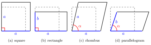
Figure 8: The four planar crystal systems. The number of lattice parameters are (a) 1, (b) 2, (c) 2, (d) 3.

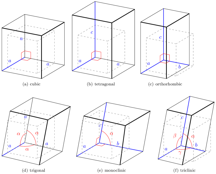
Figure 9: The six crystal systems addressed in this work. The number of lattice parameters are (a) 1, (b) 2, (c) 3, (d) 2, (e) 4, (f) 6.

The crystal system of a framework specifies the maximum number of parameters that determine the lattice, and therefore the number of lattice columns of our orbit rigidity matrix. We may further reduce the number of lattice columns by changing the type of lattice that we are considering: (flexible, distortional, scaling, hydrostatic or fixed), although it should be noted that the lattice system will partially determine these choices. For instance, for a two-dimensional framework with a rhombus unit cell, scaling and hydrostatic will be identical.

Remark 5.1

If we transform the lattice to the unit cube, by an affine transformation which preserves the symmetry, then the lattice parameters represent the number of non-zero partial derivatives of the length of bars, for variables from the lattice pattern.

The rigidity of the symmetric periodic framework can be studied using the orbit matrix. Letting $v_{0}$ and $e_{0}$ represent the number of vertices and edges in the orbit graph $G$, the orbit matrix has dimension $e_{0}\times(dv_{0}+\ell_{\mathcal{S}})$, where $\ell_{\mathcal{S}}$ describes the number of columns corresponding to the lattice parameters. This number will vary depending on a) the crystal system corresponding to the symmetry group $\mathcal{S}$, and b) the type of lattice variation we are considering (i.e. flexible, distortional, scaling, hydrostatic, or fixed).

As with the orbit matrices for ${\cal S}$, the second number which is important is the number of trivial motions which preserve all the group operations. Since we are working with periodic frameworks, we are looking for what translations also preserve the symmetries in ${\cal S}$ within the orbit matrix. We denote by $t_{{\cal S}}$ the dimension of the space of points which is fixed by all elements of the group ${\cal S}$. This space is also called the symmetry element of the group. For our calculations here, this can only be one point, a line, a plane, or all of $3$-space.

It is the combination of these two numbers $\ell_{\cal S}$ and $t_{{\cal S}}$, plus the number of orbits of edges and vertices (corresponding to the number of edges $e_{0}$ and vertices $v_{0}$ of the orbit graph $\langle G,g\rangle$), which generates the predictions of the number of non-trivial motions (if any) which occur when the vertices of the framework are in generic position. As before, we assume that no edges or vertices are fixed by the action of the group $\mathbb{Z}^{d}\rtimes{\cal S}$.

In Section 6 we describe symmetric periodic frameworks with two samples of ${\cal S}$ in the plane in detail, followed by tables covering all the groups within our analysis. In Section LABEL:sec:SpacePeriodicSymmetry we outline two samples of ${{\cal S}}$ in 3-space, again followed by tables for the relevant groups.

In the tables we give three distinct notations for each group: the Schoenflies notation used by chemists (bishop; Hall), the Hermann-Mauguin notation used internationally by crystallographers (Tables), and the orbifold notation used by mathematicians (Conway).

Recall that the Schoenflies notation was briefly introduced in Section 3.1.

In the Hermann-Mauguin notation, $n$-fold rotational symmetries are denoted by $n$, and these axis numbers are written down in decreasing order of $n$. If an $n$-fold rotational axis is contained in a mirror, then an $m$ is written after the corresponding axis number. If there exists a mirror which is perpendicular to an $n$-fold rotational axis, then this is denoted by placing the symbol $/m$ after the corresponding axis number. Finally, the notation $\overline{n}$ for an axis number $n$ indicates that an inversion, followed by the $n$-fold rotation, is a symmetry of the structure.

In the orbifold notation for wallpaper groups in the plane, an $n$-fold rotational symmetry is denoted by $n$, and a mirror symmetry is denoted by an asterisk, $*$. A number before an asterisk indicates a center of pure rotation, whereas a number after an asterisk indicates a center of rotation with mirrors through it. If there are only translational symmetries present, then this is denoted by the symbol $\circ$. The orbifold notation for groups in $3$-space is similar; note, however, that for a group in $3$-space, an $x$ indicates the presence of an inversion symmetry, whereas in $2$-space, $x$ indicates a glide reflection.

For an interdisciplinary audience, the simultaneous use of these three notations seems to be an appropriate presentation, and such comparative columns can be found in multiple sources, including the Wikipedia pages for crystal systems (Wiki).

Note that the assumption that the group has the form $\mathbb{Z}^{d}\rtimes{\cal S}$ means that we do not cover all the plane wallpaper groups, or the full set of space groups. Specifically, we will not include groups which have glide reflections as generators of the group, or those which have $6$-fold rotations. These other groups will also have orbit matrices, but require an alternative analysis for comparisons and counts. We return to this issue in Section LABEL:subsec:OtherGroups.

6 $2$-D periodic frameworks with symmetry: $\mathbb{Z}^{2}\rtimes\cal S$

6.1 $\mathbb{Z}^{2}\rtimes\mathcal{C}_{2}$ - half-turn symmetry in the plane lattice

Half-turn symmetry in the plane is equivalent to inversion in the point axis. This symmetry fits an arbitrary parallelogram for the lattice (Figure 8(d)), and $\ell_{\mathcal{C}_{2}}=3$. We will consider periodic plane frameworks with symmetry $\mathbb{Z}^{2}\rtimes\mathcal{C}_{2}$ for two variations of the lattice: (1) a fully flexible lattice; (2) a fixed lattice.

Example 6.1.1: fully flexible lattice $\mathbb{Z}^{2}\rtimes\mathcal{C}_{2}$. The original (non-symmetric) necessary count for a periodic framework on the fully flexible lattice to be minimally rigid is $e=2v+1$ (recall Theorem 4.3). To permit half-turn symmetry, with no vertex or edge fixed by the half-turn, we will need to start with the modified count $2e_{0}=2(2v_{0})+2$, where $v_{0}$ and $e_{0}$ are the numbers of vertices and edges of the orbit graph, respectively. Dividing by $2$, this gives $e_{0}=2v_{0}+1$.

Figure 10: A generically rigid graph on a fully flexible lattice, realized with 2-fold symmetry has several non-trivial flexes changing the lattice. Its periodic symmetric orbit graph is pictured in (d).

Under the half-turn symmetry with a fully flexible lattice, the orbit matrix has $2$ columns under each orbit of vertices, plus $\ell_{\mathcal{C}_{2}}=3$ columns for the three parameters for the lattice deformations. Further, we clearly have $t_{\mathcal{C}_{2}}=0$ since there are no infinitesimal trivial motions which preserve the half-turn symmetry along with the periodic lattice. This creates the necessary symmetric Maxwell condition

$$e_{0}\ \geq\ 2v_{0}+3-0$$

for periodic rigidity. However, as shown above, for a graph that was previously minimally rigid without the symmetry, we have $e_{0}=2v_{0}+1\ <\ 2v_{0}+3$. This gap predicts that a graph which counted to be minimally rigid without symmetry, realized generically with half-turn symmetry on a fully flexible lattice, now has two degrees of (finite) flexibility. As an example, consider the snapshots of three configurations with the same edge lengths but changing angles and lengths of the unit cell in Figure 10. Together these snap shots confirm the predicted two degrees of freedom.

The orbit matrix corresponding to the framework pictured in Figure 10 has the following form:

$$\begin{array}{ccccc}& p{}_1& p{}_2& p{}_3& (t{}_{11},t{}_{21},t{}_{22})\\ \{1,2\}& (p{}_1-p{}_2)& (p{}_2-p{}_1)& 0& (0,0,0)\\ \{2,3\}& 0& (p{}_2-p{}_3)& (p{}_3-p{}_2)& (0,0,0)\\ \{3,1\}& (p{}_1-p{}_3)& 0& (p{}_3-p{}_1)& (0,0,0)\\ \{1,2;g{}_1\}& (p{}_1-g{}_1(p{}_2))& (p{}_2-g{}_1{}^{-1}(p{}_1))& 0& (\ast ,\ast ,\ast )\\ \{1,2;g{}_2\}& (p{}_1-g{}_2(p{}_2))& (p{}_2-g{}_2{}^{-1}(p{}_1))& 0& (\ast ,\ast ,\ast )\\ \{2,1;g{}_3\}& (p{}_1-g{}_3{}^{-1}(p{}_2))& (p{}_2-g{}_3(p{}_1))& 0& (\ast ,\ast ,\ast )\\ \{3,1;g{}_4\}& (p{}_1-g{}_4{}^{-1}(p{}_3))& 0& (p{}_3-g{}_4(p{}_1))& (\ast ,\ast ,\ast )\end{array}$$