SUPERSYMMETRY ON THE RUN: LHC AND DARK MATTER

Abstract

Supersymmetry, a new symmetry that relates bosons and fermions in particle physics, still escapes observation. Search for SUSY is one of the main aims of the recently launched Large Hadron Collider. The other possible manifestation of SUSY is the Dark Matter in the Universe. The present lectures contain a brief introduction to supersymmetry in particle physics. The main notions of supersymmetry are introduced. The supersymmetric extension of the Standard Model - the Minimal Supersymmetric Standard Model - is considered in more detail. Phenomenological features of the MSSM as well as possible experimental signatures of SUSY at the LHC are described. The DM problem and its possible SUSY solution is presented.

1 Introduction: What is supersymmetry

Supersymmetry is a boson-fermion symmetry that is aimed to unify all forces in Nature including gravity within a singe framework [1]-[5]. Modern views on supersymmetry in particle physics are based on string paradigm, though the low energy manifestations of SUSY can be possibly found at modern colliders and in non-accelerator experiments.

Supersymmetry emerged from the attempts to generalize the Poincaré algebra to mix representations with different spin [1]. It happened to be a problematic task due to the no-go theorems preventing such generalizations [6]. The way out was found by introducing the so-called graded Lie algebras, i.e. adding the anti-commutators to the usual commutators of the Lorentz algebra. Such a generalization, described below, appeared to be the only possible one within relativistic field theory.

If $Q$ is a generator of SUSY algebra, then acting on a boson state it produces a fermion one and vice versa

$$\bar{Q}|boson\!\!>=|fermion\!\!>,\ \ Q|fermion\!\!>=|boson\!\!>\!\!.$$

Since bosons commute with each other and fermions anticommute, one immediately finds that SUSY generators should also anticommute, they must be fermionic, i.e. they must change the spin by a half-odd amount and change the statistics. The key element of SUSY algebra is

$$\{Q_{\alpha},\bar{Q}_{\dot{\alpha}}\}=2\sigma_{\alpha,\dot{\alpha}}^{\mu}P_{\mu},$$ (1.1)

where $Q$ and $\bar{Q}$ are SUSY generators and $P_{\mu}$ is the generator of translation, the four-momentum.

In what follows we describe SUSY algebra in more detail and construct its representations which are needed to build a SUSY generalization of the Standard Model of fundamental interactions. Such a generalization is based on a softly broken SUSY quantum filed theory and contains the SM as a low energy theory.

Supersymmetry promises to solve some problems of the SM and of Grand Unified Theories. In what follows we describe supersymmetry as a nearest option for the new physics on a TeV scale.

2 Motivation of SUSY in particle physics

2.1 Unification with gravity

The general idea is a unification of all forces of Nature including quantum gravity. However, the graviton has spin 2, while the other gauge bosons (photon, gluons, $W$ and $Z$ weak bosons) have spin 1. Therefore, they correspond to different representations of the Poincaré algebra. To mix them one can use supersymmetry transformations. Starting with the graviton state of spin 2 and acting by SUSY generators we get the following chain of states:

$$spin\ 2\rightarrow spin\ \frac{3}{2}\rightarrow spin\ 1\rightarrow spin\ \frac{1}{2}\rightarrow spin\ 0.$$

Thus, a partial unification of matter (fermions) with forces (bosons) naturally arises from an attempt to unify gravity with other interactions.

Taking infinitesimal transformations $\delta_{\epsilon}=\epsilon^{\alpha}Q_{\alpha},\ \bar{\delta}_{\bar{\epsilon}}=\bar{Q}_{\dot{\alpha}}{\bar{\epsilon}}^{\dot{\alpha}},$ and using eq.(1.1) one gets

$$\{\delta_{\epsilon},\bar{\delta}_{\bar{\epsilon}}\}=2(\epsilon\sigma^{\mu}\bar{\epsilon})P_{\mu},$$ (2.1)

where $\epsilon$ is a transformation parameter. Choosing $\epsilon$ to be local, i.e. a function of a space-time point $\epsilon=\epsilon(x)$, one finds from eq.(2.1) that an anticommutator of two SUSY transformations is a local coordinate translation. And a theory which is invariant under local coordinate transformation is General Relativity. Thus, making SUSY local, one naturally obtains General Relativity, or a theory of gravity, or supergravity [2].

2.2 Unification of gauge couplings

According to the Grand Unification hypothesis, gauge symmetry increases with energy [7]. All known interactions are different branches of a unique interaction associated with a simple gauge group. The unification (or splitting) occurs at high energy. To reach this goal one has to consider how the couplings change with energy. This is described by the renormalization group equations. In the SM the strong and weak couplings associated with non-Abelian gauge groups decrease with energy, while the electromagnetic one associated with the Abelian group on the contrary increases. Thus, it becomes possible that at some energy scale they become equal.

After the precise measurement of the $SU(3)\times SU(2)\times U(1)$ coupling constants, it has become possible to check the unification numerically. The three coupling constants to be compared are

$$\alpha_{1} = (5/3)g^{\prime 2}/(4\pi)=5\alpha/(3\cos^{2}\theta_{W}),$$

$$\alpha_{2} = g^{2}/(4\pi)=\alpha/\sin^{2}\theta_{W},$$ (2.2)

$$\alpha_{3} = g_{s}^{2}/(4\pi)$$

where $g^{\prime},~{}g$ and $g_{s}$ are the usual $U(1)$, $SU(2)$ and $SU(3)$ coupling constants and $\alpha$ is the fine structure constant. The factor of 5/3 in the definition of $\alpha_{1}$ has been included for proper normalization of the generators.

In the modified minimal subtraction ($\overline{MS}$) scheme, the world averaged values of the couplings at the Z⁰ energy are obtained from a fit to the LEP and Tevatron data [8]:

$$\alpha^{-1}(M_{Z}) = 128.978\pm 0.027$$

$$\sin^{2}\theta_{\overline{MS}} = 0.23146\pm 0.00017$$ (2.3)

$$\alpha_{s} = 0.1184\pm 0.0031,$$

that gives

$$\alpha_{1}(M_{Z}) = 0.017,$$

$$\alpha_{2}(M_{Z}) = 0.034,$$ (2.4)

$$\ \alpha_{3}(M_{Z}) = 0.118\pm 0.003.$$

Assuming that the SM is valid up to the unification scale, one can then use the known RG equations for the three couplings. In the leading order they are:

$$\frac{d\tilde{\alpha}_{i}}{dt}=b_{i}\tilde{\alpha}_{i}^{2},\ \ \ \ \tilde{\alpha}_{i}=\frac{\alpha_{i}}{4\pi},\ \ \ \ \ t=log(\frac{Q^{2}}{\mu^{2}}),$$ (2.5)

where for the SM the coefficients are $b_{i}=(41/10,-19/6,-7)$.

The solution to eq.(2.5) is very simple

$$\frac{1}{\tilde{\alpha}_{i}(Q^{2})}=\frac{1}{\tilde{\alpha}_{i}(\mu^{2})}-b_{i}log(\frac{Q^{2}}{\mu^{2}}).$$ (2.6)

The result is demonstrated in Fig.1 showing the evolution of the inverse of the couplings as a function of the logarithm of energy. In this presentation, the evolution becomes a straight line in first order. The second order corrections are small and do not cause any visible deviation from a straight line. Fig.1 clearly demonstrates that within the SM the coupling constant unification at a single point is impossible. It is excluded by more than 8 standard deviations. This result means that the unification can only be obtained if new physics enters between the electroweak and the Planck scales.

Figure 1: Evolution of the inverse of the three coupling constants in the Standard Model (left) and in the supersymmetric extension of the SM (MSSM) (right).

In the SUSY case, the slopes of the RG evolution curves are modified. The coefficients $b_{i}$ in eq.(2.5) now are $b_{i}=(33/5,1,-3)$. The SUSY particles are assumed to effectively contribute to the running of the coupling constants only for energies above the typical SUSY mass scale. It turns out that within the SUSY model a perfect unification can be obtained as is shown in Fig.1. From the fit requiring unification one finds for the break point $M_{SUSY}$ and the unification point $M_{GUT}$ [9]

$$M_{SUSY} = 10^{3.4\pm 0.9\pm 0.4}\ GeV,$$

$$M_{GUT} = 10^{15.8\pm 0.3\pm 0.1}\ GeV,$$ (2.7)

$$\alpha^{-1}_{GUT} = 26.3\pm 1.9\pm 1.0,$$

The first error originates from the uncertainty in the coupling constant, while the second one is due to the uncertainty in the mass splittings between the SUSY particles.

This observation was considered as the first ”evidence” for supersymmetry, especially since $M_{SUSY}$ was found in the range preferred by the fine-tuning arguments.

2.3 Solution of the hierarchy problem

The appearance of two different scales $V\gg v$ in a GUT theory, namely, $M_{W}$ and $M_{GUT}$, leads to a very serious problem which is called the hierarchy problem. There are two aspects of this problem.

The first one is the very existence of the hierarchy. To get the desired spontaneous symmetry breaking pattern, one needs

$$\begin{array}[]{cc}m_{H}\sim v\sim 10^{2}\ \ \mbox{GeV}\\ m_{\Sigma}\sim V\sim 10^{16}\ \ \mbox{GeV}\end{array}\ \ \frac{m_{H}}{m_{\Sigma}}\sim 10^{-14}\ll 1,$$ (2.8)

where $H$ and $\Sigma$ are the Higgs fields responsible for the spontaneous breaking of the $SU(2)$ and the GUT groups, respectively. The question arises of how to get so small number in a natural way.

The second aspect of the hierarchy problem is connected with the preservation of a given hierarchy. Even if we choose the hierarchy like eq.(2.8) the radiative corrections will destroy it! To see this, consider the radiative correction to the light Higgs mass given by the Feynman diagram shown in Fig.2.

Figure 2: Radiative correction to the light Higgs boson mass

This correction, proportional to the mass squared of the heavy particle, obviously, spoils the hierarchy if it is not cancelled. This very accurate cancellation with a precision $\sim 10^{-14}$ needs a fine tuning of the coupling constants.

The only known way of achieving this kind of cancellation of quadratic terms (also known as the cancellation of the quadratic divergencies) is supersymmetry. Moreover, SUSY automatically cancels quadratic corrections in all orders of PT. This is due to the contributions of superpartners of ordinary particles. The contribution from boson loops cancels those from the fermion ones because of an additional factor (-1) coming from Fermi statistics, as shown in Fig.3.

Figure 3: Cancellation of quadratic terms (divergencies)

One can see here two types of contribution. The first line is the contribution of the heavy Higgs boson and its superpartner. The strength of interaction is given by the Yukawa coupling $\lambda$. The second line represents the gauge interaction proportional to the gauge coupling constant $g$ with the contribution from the heavy gauge boson and heavy gaugino.

In both the cases the cancellation of quadratic terms takes place. This cancellation is true up to the SUSY breaking scale, $M_{SUSY}$, which should not be very large ($\leq$ 1 TeV) to make the fine-tuning natural. Indeed, let us take the Higgs boson mass. Requiring for consistency of perturbation theory that the radiative corrections to the Higgs boson mass do not exceed the mass itself gives

$$\delta M_{h}^{2}\sim g^{2}M^{2}_{SUSY}\sim M_{h}^{2}.$$ (2.9)

So, if $M_{h}\sim 10^{2}$ GeV and $g\sim 10^{-1}$, one needs $M_{SUSY}\sim 10^{3}$ GeV in order that the relation (2.9) is valid. Thus, we again get the same rough estimate of $M_{SUSY}\sim$ 1 TeV as from the gauge coupling unification above.

That is why it is usually said that supersymmetry solves the hierarchy problem. We show below how SUSY can also explain the origin of the hierarchy.

2.4 Astrophysics and Cosmology

The shining matter is not the only one in the Universe. Considerable amount consists of the so-called dark matter. The direct evidence for the presence of the dark matter are the rotation curves of galaxies [10] (see Fig.4). To explain these curves one has to assume the existence of galactic halo made of non-shining matter which takes part in gravitational interaction.

Figure 4: Roration curves for the solar system and galaxy

There are two possible types of the dark matter: the hot one, consisting of light relativistic particles and the cold one, consisting of massive weakly interacting particles (WIMPs) [11]. The hot dark matter might consist of neutrinos, however, this has problems with galaxy formation. As for the cold dark matter, it has no candidates within the SM. At the same time, SUSY provides an excellent candidate for the cold dark matter, namely neutralino, the lightest superparticle [12].

2.5 Beyond GUTs: superstring

Another motivation for supersymmetry follows from even more radical changes of basic ideas related to the ultimate goal of construction of consistent unified theory of everything. At the moment the only viable conception is the superstring theory [13]. In the superstring theory, strings are considered as fundamental objects, closed or open, and are nonlocal in nature. Ordinary particles are considered as string excitation modes. String interactions, which are local, generate proper interactions of usual particles, including gravitational ones.

To be consistent, the string theory should be conformal invariant in D-dimensional target space and have a stable vacuum. The first requirement is valid in classical theory but may be violated by quantum anomalies. Cancellation of quantum anomalies takes place when space-time dimension of a target space equals to a critical one which is $D_{c}=26$ for bosonic string and $D_{c}=10$ for a fermionic one.

The second requirement is that the massless string excitations (the particles of the SM) are stable. This assumes the absence of tachyons, the states with imaginary mass, which can be guaranteed only in supersymmetric string theories!

3 Basics of supersymmetry

3.1 Algebra of SUSY

Combined with the usual Poincaré and internal symmetry algebra the Super-Poincaré Lie algebra contains additional SUSY generators $Q_{\alpha}^{i}$ and $\bar{Q}_{\dot{\alpha}}^{i}$ [3]

$${[}P_{\mu},P_{\nu}{]}=0,$$

$${[}P_{\mu},M_{\rho\sigma}{]}=i(g_{\mu\rho}P_{\sigma}-g_{\mu\sigma}P_{\rho}),$$

$${[}M_{\mu\nu},M_{\rho\sigma}{]}\!=\!i(\!g_{\nu\rho}M_{\mu\sigma}\!\!-\!\!g_{\nu\sigma}M_{\mu\rho}\!\!-\!\!g_{\mu\rho}M_{\nu\sigma}\!\!+\!\!g_{\mu\sigma}M_{\nu\rho}\!),$$

$${[}B_{r},B_{s}{]}=iC_{rs}^{t}B_{t},$$

$${[}B_{r},P_{\mu}{]}={[}B_{r},M_{\mu\sigma}{]}=0,$$ (3.1)

$${[}Q_{\alpha}^{i},P_{\mu}{]}={[}\bar{Q}_{\dot{\alpha}}^{i},P_{\mu}{]}=0,$$

$${[}Q_{\alpha}^{i},M_{\mu\nu}{]}\!=\!\frac{1}{2}(\!\sigma_{\mu\nu}\!)_{\alpha}^{\beta}Q_{\beta}^{i},\!\ {[}\bar{Q}_{\dot{\alpha}}^{i},M_{\mu\nu}{]}\!=\!\frac{-1}{2}\bar{Q}_{\dot{\beta}}^{i}(\!\bar{\sigma}_{\mu\nu}\!)_{\dot{\alpha}}^{\dot{\beta}},$$

$${[}Q_{\alpha}^{i},B_{r}{]}=(b_{r})_{j}^{i}Q_{\alpha}^{j},\ \ \ {[}\bar{Q}_{\dot{\alpha}}^{i},B_{r}{]}=-\bar{Q}_{\dot{\alpha}}^{j}(b_{r})_{j}^{i},$$

$$\{Q_{\alpha}^{i},\bar{Q}_{\dot{\beta}}^{j}\}=2\delta^{ij}(\sigma^{\mu})_{\alpha\dot{\beta}}P_{\mu},$$

$$\{Q_{\alpha}^{i},Q_{\beta}^{j}\}=2\epsilon_{\alpha\beta}Z^{ij},\ \ \ Z_{ij}=a_{ij}^{r}b_{r},\ \ Z^{ij}=Z_{ij}^{+},$$

$$\{\bar{Q}_{\dot{\alpha}}^{i},\bar{Q}_{\dot{\beta}}^{j}\}=-2\epsilon_{\dot{\alpha}\dot{\beta}}Z^{ij},\ \ \ {[}Z_{ij},anything{]}=0,$$

$$\alpha,\dot{\alpha}=1,2\ \ \ \ i,j=1,2,\ldots,N.$$

Here $P_{\mu}$ and $M_{\mu\nu}$ are four-momentum and angular momentum operators, respectively, $B_{r}$ are the internal symmetry generators, $Q^{i}$ and $\bar{Q}^{i}$ are the spinorial SUSY generators and $Z_{ij}$ are the so-called central charges; $\alpha,\dot{\alpha},\beta,\dot{\beta}$ are the spinorial indices. In the simplest case one has one spinor generator $Q_{\alpha}$ (and the conjugated one $\bar{Q}_{\dot{\alpha}}$) that corresponds to an ordinary or N=1 supersymmetry. When $N>1$ one has an extended supersymmetry.

A natural question arises: how many SUSY generators are possible, i.e. what is the value of $N$? To answer this question, consider massless states. Let us start with the ground state labeled by energy and helicity, i.e. projection of a spin on the direction of momenta, and let it be annihilated by $Q_{i}$

$${\rm Vacuum}=|E,\lambda>,\ \ \ \ \ \ \ Q_{i}|E,\lambda>=0.$$

Then one and more particle states can be constructed with the help of a creation operators as

$$\begin{array}[]{lll}\mbox{\text@underline{State}}&\mbox{\text@underline{Expression}}&\#\ \mbox{ \text@underline{of States}}\\ \\ \mbox{vacuum}&|E,\lambda\!>&1\\ 1\!-\!\mbox{particle}&\bar{Q}_{i}|E,\lambda\!>=|E,\lambda\!+\!1/2\!>_{i}&N\\ 2\!-\!\mbox{particle}&\bar{Q}_{i}\bar{Q}_{j}|E,\lambda\!>=|E,\lambda\!+\!1\!>_{ij}&\frac{N(N-1)}{2}\\ ...&...&...\\ N\!-\!\mbox{particle}&\bar{Q}_{1}...\bar{Q}_{N}|E,\lambda\!>=|E,\lambda\!+\!\frac{N}{2}\!\!>&1\end{array}$$

Total $\#$ of states: $\displaystyle\sum_{k=0}^{N}\left(\begin{array}[]{c}N\\ k\end{array}\right)=2^{N}=2^{N-1}$ bosons + $2^{N-1}$ fermions. The energy $E$ is not changed, since according to (3.1) the operators $\bar{Q}_{i}$ commute with the Hamiltonian.

Thus, one has a sequence of bosonic and fermionic states and the total number of bosons equals that of fermions. This is a generic property of any supersymmetric theory. However, in CPT invariant theories the number of states is doubled, since CPT transformation changes the sign of helicity. Hence, in CPT invariant theories, one has to add the states with opposite helicity to the above mentioned ones.

Consider some examples. Let us take $N=1$ and $\lambda=0$. Then one has the following set of states:

$$\begin{array}[]{lllllc}N=1&\lambda=0&&&&\\ \mbox{helicity}&0\ \frac{1}{2}&&\mbox{helicity}&0\ -\frac{1}{2}\\ &&\stackrel{{\scriptstyle CPT}}{{\Longrightarrow}}&&\\ \#\ \mbox{of states}&1\ 1&&\#\ \mbox{of states}&1\ \ \ \ 1\end{array}$$

Hence, a complete $N=1$ multiplet is

$$\begin{array}[]{llccc}N=1&\mbox{helicity}&-1/2&0&1/2\\ &\#\ \mbox{of states}&\ 1&2&1\end{array}$$

which contains one complex scalar and one spinor with two helicity states.

This is an example of the so-called self-conjugated multiplet. There are also self-conjugated multiplets with $N>1$ corresponding to extended supersymmetry. Two particular examples are the $N=4$ super Yang-Mills multiplet and the $N=8$ supergravity multiplet

$$N=4\ \ \ \mbox{SUSY YM}\ \ \ \lambda=-1$$

$$\begin{array}[]{cccccccccc}\mbox{helicity}&&&-1&-1/2&0&1/2&1&&\\ \#\ \mbox{of states}&&&\ \ 1&\ 4&6&4&1&&\\ \end{array}$$

$$N=8\ \ \ \mbox{SUGRA}\ \ \ \lambda=-2$$

$$\begin{array}[]{ccccccccc}-2&-3/2&-1&-1/2&0&1/2&1&3/2&2\\ 1&8&28&56&70&56&28&8&1\end{array}$$

One can see that the multiplets of extended supersymmetry are very rich and contain a vast number of particles.

The constraint on the number of SUSY generators comes from a requirement of consistency of the corresponding QFT. The number of supersymmetries and the maximal spin of the particle in the multiplet are related by

$$N\leq 4S,$$

where $S$ is the maximal spin. Since the theories with spin greater than 1 are non-renormalizable and the theories with spin greater than 5/2 have no consistent coupling to gravity, this imposes a constraint on the number of SUSY generators

$$\begin{array}[]{cl}N\leq 4&\ \ \ \ \mbox{for renormalizable theories (YM),}\\ N\leq 8&\ \ \ \ \mbox{for (super)gravity}.\end{array}$$

In what follows, we shall consider simple supersymmetry, or $N=1$ supersymmetry, contrary to extended supersymmetries with $N>1$. In this case, one has the following types of supermultiplets which are used in the construction of SUSY generalization of the SM

$$\begin{array}[]{ll}\hskip 34.14322pt(\phi,\ \ \psi)&\hskip 28.45274pt(\lambda,\ \ A_{\mu})\\ Spin=0,\ Spin=1/2&Spin=1/2,\ Spin=1\\ \ \ scalar\ \ \ \ \ \ chiral&majorana\ \ \ \ vector\\ \hskip 48.36958ptfermion&fermion\end{array}$$

each of them contains two physical states, one boson and one fermion. They are called chiral and vector multiplets, respectively. Construction the generalization of the SM one has to put all the particles into these multiplets. For instance, quarks should go into chiral multiplet and photon into vector multiplet.

3.2 Superspace and supermultiplets

An elegant formulation of supersymmetry transformations and invariants can be achieved in the framework of superspace [4]. Superspace differs from the ordinary Euclidean (Minkowski) space by adding of two new coordinates, $\theta_{\alpha}$ and $\bar{\theta}_{\dot{\alpha}}$, which are Grassmannian, i.e. anticommuting, variables

$$\{\theta_{\alpha},\theta_{\beta}\}=0,\ \ \{\bar{\theta}_{\dot{\alpha}},\bar{\theta}_{\dot{\beta}}\}=0,\ \ \theta_{\alpha}^{2}=0,\ \ \bar{\theta}_{\dot{\alpha}}^{2}=0,$$

$$\alpha,\beta,\dot{\alpha},\dot{\beta}=1,2.$$

Thus, we go from space to superspace

$$\begin{array}[]{cc}Space&\ \Rightarrow\ \ Superspace\\ x_{\mu}&\ \ \ \ \ \ \ x_{\mu},\theta_{\alpha},\bar{\theta}_{\dot{\alpha}}\end{array}$$

A SUSY group element can be constructed in superspace in the same way as an ordinary translation in the usual space

$$G(x,\theta,\bar{\theta})=e^{\displaystyle i(-x^{\mu}P_{\mu}+\theta Q+\bar{\theta}\bar{Q})}.$$ (3.2)

It leads to a supertranslation in superspace

$$\begin{array}[]{ccl}x_{\mu}&\rightarrow&x_{\mu}+i\theta\sigma_{\mu}\bar{\varepsilon}-i\varepsilon\sigma_{\mu}\bar{\theta},\\ \theta&\rightarrow&\theta+\varepsilon,\ \ \bar{\theta}\rightarrow\bar{\theta}+\bar{\varepsilon},\end{array}$$ (3.3)

where $\varepsilon$ and $\bar{\varepsilon}$ are Grassmannian transformation parameters. From eq.(3.3) one can easily obtain the representation for the supercharges (3.1) acting on the superspace

$$Q_{\alpha}\!=\!\frac{\partial}{\partial\theta_{\alpha}}\!-\!i\sigma^{\mu}_{\alpha\dot{\alpha}}\bar{\theta}^{\dot{\alpha}}\partial_{\mu},\ \bar{Q}_{\dot{\alpha}}\!=\!\frac{-\partial}{\partial\bar{\theta}_{\dot{\alpha}}}\!+\!i\theta_{\alpha}\sigma^{\mu}_{\alpha\dot{\alpha}}\partial_{\mu}.$$ (3.4)

Working in superspace all the fields become functions of not only the space-time point $x_{\mu}$ but also the Grassmanian coordinates $\theta$, i.e. they become superfields. The superfield contains inside the whole supermultiplet. We will not describe the superfields here and refer the reader to existing literature. What is important for us is that this formalizm is straightforward and allows one to construct a SUSY generalization of any theory.

4 SUSY generalization of the Standard Model. The MSSM

As has been already mentioned, in SUSY theories the number of bosonic degrees of freedom equals that of fermionic. At the same time, in the SM one has 28 bosonic and 90 fermionic degrees of freedom (with massless neutrino, otherwise 96). So the SM is to a great extent non-supersymmetric. Trying to add some new particles to supersymmetrize the SM, one should take into account the following observations:

$\bullet$ There are no fermions with quantum numbers of the gauge bosons;

$\bullet$ Higgs fields have nonzero v.e.v.s; hence they cannot be superpartners of quarks and leptons since this would induce spontaneous violation of baryon and lepton numbers;

$\bullet$ One needs at least two complex chiral Higgs multiplets to give masses to Up and Down quarks.

The latter is due to the form of a superpotential and chirality of matter superfields. Indeed, the superpotential should be invariant under the $SU(3)\times SU(2)\times U(1)$ gauge group. If one looks at the Yukawa interaction in the Standard Model, one finds that it is indeed $U(1)$ invariant since the sum of hypercharges in each vertex equals zero. For the up quarks this is achieved by taking the conjugated Higgs doublet $\tilde{H}=i\tau_{2}H^{\dagger}$ instead of $H$. However, in SUSY $H$ is a chiral superfield and hence a superpotential, which is constructed out of chiral fields, can contain only $H$ but not $\tilde{H}$ which is an antichiral superfield.

Another reason for the second Higgs doublet is related to chiral anomalies. It is known that chiral anomalies spoil the gauge invariance and, hence, the renormalizability of the theory. They are canceled in the SM between quarks and leptons in each generation [14]

$$\begin{array}[]{l}TrY^{3}=3\ (\frac{1}{27}+\frac{1}{27}-\frac{64}{27}+\frac{8}{27})-1-1+8=0\\ \hskip 22.76228ptcolor\ \ u_{L}\ \ \ d_{L}\ \ \ \ u_{R}\ \ d_{R}\hskip 14.22636pt\nu_{L}\ \ e_{L}\ \ e_{R}\end{array}$$

However, if one introduces a chiral Higgs superfield, it contains higgsinos, which are chiral fermions, and contain anomalies. To cancel them one has to add the second Higgs doublet with the opposite hypercharge. Therefore, the Higgs sector in SUSY models is inevitably enlarged, it contains an even number of doublets.

Conclusion: In SUSY models supersymmetry associates known bosons with new fermions and known fermions with new bosons.

4.1 The field content

Consider the particle content of the Minimal Supersymmetric Standard Model [15, 16]. According to the previous discussion, in the minimal version we double the number of particles (introducing a superpartner to each particle) and add another Higgs doublet (with its superpartner).

Thus, the characteristic feature of any supersymmetric generalization of the SM is the presence of superpartners (see Fig.5) [17]. If supersymmetry is exact, superpartners of ordinary particles should have the same masses and have to be observed. The absence of them at modern energies is believed to be explained by the fact that their masses are very heavy, that means that supersymmetry should be broken. Hence, if the energy of accelerators is high enough, the superpartners will be created.

Figure 5: The shadow world of SUSY particles

The particle content of the MSSM then appears as shown in the table.

Particle Content of the MSSM

Superfield	Bosons	Fermions	$SU(3)$	$SU(2$	$U_{Y}(1)$
Gauge
${\bf G^{a}}$	gluon                 $g^{a}$	gluino$\ \ \ \ \ \ \ \ \ \ \ \ \tilde{g}^{a}$	8	0	0
${\bf V^{k}}$	Weak    $W^{k}$  $(W^{\pm},Z)$	wino, zino  $\tilde{w}^{k}$  $(\tilde{w}^{\pm},\tilde{z})$	1	3	0
${\bf V^{\prime}}$	Hypercharge    $B\ (\gamma)$	bino            $\tilde{b}(\tilde{\gamma})$	1	1	0
Matter
$\begin{array}[]{c}{\bf L_{i}}\\ {\bf E_{i}}\end{array}$	sleptons  $\left\{\begin{array}[]{l}\tilde{L}_{i}=(\tilde{\nu},\tilde{e})_{L}\\ \tilde{E}_{i}=\tilde{e}_{R}\end{array}\right.$	leptons  $\left\{\begin{array}[]{l}L_{i}=(\nu,e)_{L}\\ E_{i}=e_{R}^{c}\end{array}\right.$	$\begin{array}[]{l}1\\ 1\end{array}$	$\begin{array}[]{l}2\\ 1\end{array}$	$\begin{array}[]{r}-1\\ 2\end{array}$
$\begin{array}[]{c}{\bf Q_{i}}\\ {\bf U_{i}}\\ {\bf D_{i}}\end{array}$	squarks  $\left\{\begin{array}[]{l}\tilde{Q}_{i}=(\tilde{u},\tilde{d})_{L}\\ \tilde{U}_{i}=\tilde{u}_{R}\\ \tilde{D}_{i}=\tilde{d}_{R}\end{array}\right.$	quarks  $\left\{\begin{array}[]{l}Q_{i}=(u,d)_{L}\\ U_{i}=u_{R}^{c}\\ D_{i}=d_{R}^{c}\end{array}\right.$	$\begin{array}[]{l}3\\ 3^{*}\\ 3^{*}\end{array}$	$\begin{array}[]{l}2\\ 1\\ 1\end{array}$	$\begin{array}[]{r}1/3\\ -4/3\\ 2/3\end{array}$
Higgs
$\begin{array}[]{c}{\bf H_{1}}\\ {\bf H_{2}}\end{array}$	Higgses  $\left\{\begin{array}[]{l}H_{1}\\ H_{2}\end{array}\right.$	higgsinos  $\left\{\begin{array}[]{l}\tilde{H}_{1}\\ \tilde{H}_{2}\end{array}\right.$	$\begin{array}[]{l}1\\ 1\end{array}$	$\begin{array}[]{l}2\\ 2\end{array}$	$\begin{array}[]{r}-1\\ 1\end{array}$

Hereafter, tilde denotes a superpartner of an ordinary particle.

The presence of an extra Higgs doublet in SUSY model is a novel feature of the theory. In the MSSM one has two doublets with the quantum numbers (1,2,-1) and (1,2,1), respectively:

$$H_{1} = \left(\begin{array}[]{c}H^{0}_{1}\\ H_{1}^{-}\end{array}\right)=\left(\begin{array}[]{c}v_{1}+\frac{S_{1}+iP_{1}}{\sqrt{2}}\\ H^{-}_{1}\end{array}\right),$$

$$H_{2} = \left(\begin{array}[]{c}H^{+}_{2}\\ H_{2}^{0}\end{array}\right)=\left(\begin{array}[]{c}H^{+}_{2}\\ v_{2}+\frac{S_{2}+iP_{2}}{\sqrt{2}}\end{array}\right),$$

where $v_{i}$ are the vacuum expectation values of the neutral components.

Hence, one has 8=4+4=5+3 degrees of freedom. As in the case of the SM, 3 degrees of freedom can be gauged away, and one is left with 5 physical states compared to 1 in the SM. Thus, in the MSSM, as actually in any of two Higgs doublet models, one has five physical Higgs bosons: two CP-even neutral, one CP-odd neutral and two charged. We consider the mass eigenstates below.

4.2 Lagrangian of the MSSM

To construct a SUSY Lagrangian one has to follow the following three steps:

• $1^{st}$ step: Take your favorite Lagrangian written in terms of fields

• $2^{nd}$ step: Replace the fields ($\phi,\psi,A_{\mu}$) by superfields $\Phi,V$

• $3^{rd}$ step: Replace the Action by superAction

  $$A=\int d^{4}x{\cal L}(x)\ \ \Rightarrow\ \ A=\int d^{4}x\ d^{4}\theta{\cal L}(x,\theta,\bar{\theta})$$

At the last step one has to perform the integration over the Grassmannian variables. The rules of integration are very easy [18]:

$$\int d\theta_{\alpha}=0,\ \ \int\theta_{\alpha}d\theta_{\beta}=\delta_{\alpha,\beta}.$$

Now we can construct the Lagrangian of the MSSM. It consists of two parts; the first part is the SUSY generalization of the Standard Model, while the second one represents the SUSY breaking as mentioned above.

$${\cal L}={\cal L}_{SUSY}+{\cal L}_{Breaking},$$ (4.3)

where

$${\cal L}_{SUSY}={\cal L}_{Gauge}+{\cal L}_{Yukawa}.$$ (4.4)

We will not describe the gauge part since it is essentially the gauge invariant kinetic terms but rather concentrate on Yukawa terms. They are given by the so-called superpotential which is nothing else but the usual Yukawa terms with the fields replaced by superfields as explained above.

$${\cal L}_{Yukawa}=\epsilon_{ij}(y^{U}_{ab}Q_{a}^{j}U^{c}_{b}H_{2}^{i}+y^{D}_{ab}Q_{a}^{j}D^{c}_{b}H_{1}^{i}$$

$$+y^{L}_{ab}L_{a}^{j}E^{c}_{b}H_{1}^{i}+\mu H_{1}^{i}H_{2}^{j}),$$ (4.5)

where $i,j=1,2$ are the $SU(2)$ and $a,b=1,2,3$ are the generation indices; colour indices are suppressed. This part of the Lagrangian almost exactly repeats that of the SM. The only difference is the last term which describes the Higgs mixing. It is absent in the SM since there is only one Higgs field there.

However, one can write down the other Yukawa terms

$${\cal L}_{Yukawa}=\epsilon_{ij}(\lambda^{L}_{abd}L_{a}^{i}L_{b}^{j}E_{d}^{c}+\lambda^{L\prime}_{abd}L_{a}^{i}Q_{b}^{j}D_{d}^{c}$$

$$+\mu^{\prime}_{a}L^{i}_{a}H_{2}^{j})+\lambda^{B}_{abd}U_{a}^{c}D_{b}^{c}D_{d}^{c}.$$ (4.6)

These terms are absent in the SM. The reason is very simple: one can not replace the superfields in eq.(4.6) by the ordinary fields like in eq.(4.5) because of the Lorentz invariance. These terms have a different property, they violate either lepton (the first 3 terms in eq.(4.6)) or baryon number (the last term). Since both effects are not observed in Nature, these terms must be suppressed or excluded. One can avoid such terms introducing a special symmetry called $R$-symmetry[19]. This is the global $U(1)_{R}$ invariance

$$U(1)_{R}:\ \ \theta\to e^{i\alpha}\theta,\ \ \Phi\to e^{in\alpha}\Phi,$$ (4.7)

which is reduced to the discrete group $Z_{2}$, called the $R$-parity. The $R$-parity quantum number is given by $R=(-1)^{3(B-L)+2S}$ for particles with spin $S$. Thus, all the ordinary particles have the $R$-parity quantum number equal to $R=+1$, while all the superpartners have $R$-parity quantum number equal to $R=-1$. The first part of the Yukawa Lagrangian is R-symmetric, while the second part is R-nonsymmetric. The $R$-parity obviously forbids the terms. However, it may well be that these terms are present, though experimental limits on the couplings are very severe

$$\lambda^{L}_{abc},\ \ \lambda^{L\prime}_{abc}<10^{-4},\ \ \ \ \ \lambda^{B}_{abc}<10^{-9}.$$

4.3 Properties of interactions

If one assumes that the $R$-parity is preserved, then the interactions of superpartners are essentially the same as in the SM, but two of three particles involved into an interaction at any vertex are replaced by superpartners. The reason for it is the $R$-parity. Conservation of the $R$-parity has two consequences

$\bullet$ the superpartners are created in pairs;

$\bullet$ the lightest superparticle (LSP) is stable. Usually it is photino $\tilde{\gamma}$, the superpartner of a photon with some admixture of neutral higgsino.

Typical vertices are shown in Figs.6. The tilde above a letter denotes the corresponding superpartner. Note that the coupling is the same in all the vertices involving superpartners.

Figure 6: Gauge-matter interaction, Gauge self-interaction and Yukawa-type interaction

4.4 Creation and decay of superpartners

The above-mentioned rule together with the Feynman rules for the SM enables one to draw diagrams describing creation of superpartners. One of the most promising processes is the $e^{+}e^{-}$ annihilation (see Fig.7).

Figure 7: Creation of superpartners at electron-positron colliders

Figure 8: Gluon fusion, $q\bar{q}$ scattering, quark-gluon scattering

The usual kinematic restriction is given by the c.m. energy $m^{max}_{sparticle}\leq\frac{\sqrt{s}}{2}.\$ Similar processes take place at hadron colliders with electrons and positrons being replaced by quarks and gluons.

Experimental signatures at hadron colliders are similar to those at $e^{+}e^{-}$ machines; however, here one has much wider possibilities. Besides the usual annihilation channel, one has numerous processes of gluon fusion, quark-antiquark and quark-gluon scattering (see Fig.8).

Creation of superpartners can be accompanied by creation of ordinary particles as well. We consider various experimental signatures below. They crucially depend on SUSY breaking pattern and on the mass spectrum of superpartners.

The decay properties of superpartners also depend on their masses. For the quark and lepton superpartners the main processes are shown in Fig.9.

Figure 9: Decay of superpartners

5 Breaking of SUSY in the MSSM

Usually it is assumed that supersymmetry is broken spontaneously via the v.e.v.s of some fields. However, in the case of supersymmetry one can not use the scalar fields like the Higgs field, but rather the auxiliary fields present in any SUSY multiplet. There are two basic mechanisms of spontaneous SUSY breaking: the Fayet-Iliopoulos (or D-type) mechanism [20] based on the $D$ auxiliary field from a vector multiplet and the O’Raifeartaigh (or F-type) mechanism [21] based on the $F$ auxiliary field from a chiral multiplet. Unfortunately, one can not explicitly use these mechanisms within the MSSM since none of the fields of the MSSM can develop non-zero v.e.v. without spoiling the gauge invariance. Therefore, a spontaneous SUSY breaking should take place via some other fields.

The most common scenario for producing low-energy supersymmetry breaking is called the hidden sector one [22]. According to this scenario, there exist two sectors: the usual matter belongs to the ”visible” one, while the second, ”hidden” sector, contains fields which lead to breaking of supersymmetry. These two sectors interact with each other by exchange of some fields called messengers, which mediate SUSY breaking from the hidden to the visible sector. There might be various types of messenger fields: gravity, gauge, etc. The hidden sector is the weakest part of the MSSM. It contains a lot of ambiguities and leads to uncertainties of the MSSM predictions considered below.

So far there are known four main mechanisms to mediate SUSY breaking from a hidden to a visible sector:

• Gravity mediation (SUGRA) [23];
  

• Gauge mediation [24];
  

• Anomaly mediation [25];
  

• Gaugino mediation [26].

All four mechanisms of soft SUSY breaking are different in details but are common in results. Predictions for the sparticle spectrum depend on the mechanism of SUSY breaking. In what follows, to calculate the mass spectrum of superpartners, we need an explicit form of SUSY breaking terms. For the MSSM and without the $R$-parity violation one has in general

$$-{\cal L}_{Breaking}=$$ (5.1)

$$=\sum_{i}m^{2}_{0i}|\varphi_{i}|^{2}+\left(\frac{1}{2}\sum_{\alpha}M_{\alpha}\tilde{\lambda}_{\alpha}\tilde{\lambda}_{\alpha}+BH_{1}H_{2}\right.$$

$$+\left.A^{U}_{ab}\tilde{Q}_{a}\tilde{U}^{c}_{b}H_{2}+A^{D}_{ab}\tilde{Q}_{a}\tilde{D}^{c}_{b}H_{1}+A^{L}_{ab}\tilde{L}_{a}\tilde{E}^{c}_{b}H_{1}\right),$$

where we have suppressed the $SU(2)$ indices. Here $\varphi_{i}$ are all scalar fields, $\tilde{\lambda}_{\alpha}$ are the gaugino fields, $\tilde{Q},\tilde{U},\tilde{D}$ and $\tilde{L},\tilde{E}$ are the squark and slepton fields, respectively, and $H_{1,2}$ are the SU(2) doublet Higgs fields.

Eq.(5.1) contains a vast number of free parameters which spoils the prediction power of the model. To reduce their number, we adopt the so-called universality hypothesis, i.e., we assume the universality or equality of various soft parameters at a high energy scale, namely, we put all the spin 0 particle masses to be equal to the universal value $m_{0}$, all the spin 1/2 particle (gaugino) masses to be equal to $m_{1/2}$ and all the cubic and quadratic terms, proportional to $A$ and $B$, to repeat the structure of the Yukawa superpotential (4.5). This is an additional requirement motivated by the supergravity mechanism of SUSY breaking. Universality is not a necessary requirement and one may consider nonuniversal soft terms as well. However, it will not change the qualitative picture presented below; so for simplicity, in what follows we consider the universal boundary conditions. In this case, eq.(5.1) takes the form

$$-{\cal L}_{Breaking}=$$ (5.2)

$$=m_{0}^{2}\sum_{i}|\varphi_{i}|^{2}+\left(\frac{m_{1/2}}{2}\sum_{\alpha}\tilde{\lambda}_{\alpha}\tilde{\lambda}_{\alpha}\right.+B[\mu H_{1}H_{2}]$$

$$\left.+\ A[y^{U}_{ab}\tilde{Q}_{a}\tilde{U}^{c}_{b}H_{2}+y^{D}_{ab}\tilde{Q}_{a}\tilde{D}^{c}_{b}H_{1}+y^{L}_{ab}\tilde{L}_{a}\tilde{E}^{c}_{b}H_{1}]\right).$$

Thus, we are left with five free parameters, namely, $m_{0},m_{1/2},A,B$ and $\mu$ versus two parameters of the SM coming from the Higgs potential, $m^{2}$ and $\lambda$. In supersymmetry the Higgs potential is not arbitrary but is calculated from the Yuakawa and gauge terms as we shall see below.

The soft terms explicitly break supersymmetry. As will be shown later, they lead to the mass spectrum of superpartners different from that of ordinary particles. Remind that the masses of quarks and leptons remain zero until $SU(2)$ invariance is spontaneously broken.

5.1 The soft terms and the mass formulas

There are two main sources of the mass terms in the Lagrangian: the $D$ terms and soft ones. With given values of $m_{0},m_{1/2},\mu,Y_{t},Y_{b},Y_{\tau},A$, and $B$ one can construct the mass matrices for all the particles. Knowing them at the GUT scale, one can solve the corresponding RG equations, thus linking the values at the GUT and electroweak scales. Substituting these parameters into the mass matrices, one can predict the mass spectrum of superpartners [27, 28].

5.1.1 Gaugino-higgsino mass terms

The mass matrix for gauginos, the superpartners of the gauge bosons, and for higgsinos, the superpartners of the Higgs bosons, is nondiagonal, thus leading to their mixing. The mass terms look like

$${\cal L}_{Gaugino-Higgsino}=$$ (5.3)

$$= -\frac{1}{2}M_{3}\bar{\lambda}_{a}\lambda_{a}-\frac{1}{2}\bar{\chi}M^{(0)}\chi-(\bar{\psi}M^{(c)}\psi+h.c.),$$

where $\lambda_{a},a=1,2,\ldots,8,$ are the Majorana gluino fields and

$$\chi=\left(\begin{array}[]{c}\tilde{B}^{0}\\ \tilde{W}^{3}\\ \tilde{H}^{0}_{1}\\ \tilde{H}^{0}_{2}\end{array}\right),\ \ \ \psi=\left(\begin{array}[]{c}\tilde{W}^{+}\\ \tilde{H}^{+}\end{array}\right)$$ (5.4)

are, respectively, the Majorana neutralino and Dirac chargino fields.

The neutralino mass matrix is

$$M^{(0)}\!\!=\!\!\left(\!\begin{tabular}[]{cccc}$M_{1}$&$0$&-$M_{Z}c_{\beta}s_{W}$&$M_{Z}s_{\beta}s_{W}$\\ $0$&$M_{2}$&$M_{Z}c_{\beta}c_{W}$&-$M_{Z}s_{\beta}c_{W}$\\ -$M_{Z}c_{\beta}s_{W}$&$M_{Z}c_{\beta}c_{W}$&$0$&-$\mu$\\ $M_{Z}s_{\beta}s_{W}$&-$M_{Z}s_{\beta}c_{W}$&-$\mu$&$0$\end{tabular}\!\right),$$

where $\tan\beta=v_{2}/v_{1}$ is the ratio of two Higgs v.e.v.s and $\sin_{W}=\sin\theta_{W}$ is the usual sinus of the weak mixing angle. The physical neutralino masses $M_{\tilde{\chi}_{i}^{0}}$ are obtained as eigenvalues of this matrix after diagonalization.

For charginos one has

$$M^{(c)}=\left(\begin{array}[]{cc}M_{2}&\sqrt{2}M_{W}\sin\beta\\ \sqrt{2}M_{W}\cos\beta&\mu\end{array}\right).$$ (5.5)

This matrix has two chargino eigenstates $\tilde{\chi}_{1,2}^{\pm}$ with mass eigenvalues

$$M^{2}_{1,2} = \frac{1}{2}\left[M^{2}_{2}+\mu^{2}+2M^{2}_{W}\mp\right.$$

$$\left.\sqrt{(M^{2}_{2}\!\!-\!\!\mu^{2})^{2}\!\!+\!\!4M^{4}_{W}c^{2}_{2\beta}\!\!+\!\!4M^{2}_{W}(\!M^{2}_{2}\!+\!\mu^{2}\!\!+\!\!2M_{2}\mu s_{2\beta}\!)}\right].$$

5.1.2 Squark and slepton masses

Non-negligible Yukawa couplings cause a mixing between the electroweak eigenstates and the mass eigenstates of the third generation particles. The mixing matrices for $\tilde{m}^{2}_{t},\tilde{m}^{2}_{b}$ and $\tilde{m}^{2}_{\tau}$ are

$$\left(\begin{array}[]{cc}\tilde{m}_{tL}^{2}&m_{t}(A_{t}-\mu\cot\beta)\\ m_{t}(A_{t}-\mu\cot\beta)&\tilde{m}_{tR}^{2}\end{array}\right),$$

$$\left(\begin{array}[]{cc}\tilde{m}_{bL}^{2}&m_{b}(A_{b}-\mu\tan\beta)\\ m_{b}(A_{b}-\mu\tan\beta)&\tilde{m}_{bR}^{2}\end{array}\right),$$

$$\left(\begin{array}[]{cc}\tilde{m}_{\tau L}^{2}&m_{\tau}(A_{\tau}-\mu\tan\beta)\\ m_{\tau}(A_{\tau}-\mu\tan\beta)&\tilde{m}_{\tau R}^{2}\end{array}\right)$$

with

$$\tilde{m}_{tL}^{2} = \tilde{m}_{Q}^{2}+m_{t}^{2}+\frac{1}{6}(4M_{W}^{2}-M_{Z}^{2})\cos 2\beta,$$

$$\tilde{m}_{tR}^{2} = \tilde{m}_{U}^{2}+m_{t}^{2}-\frac{2}{3}(M_{W}^{2}-M_{Z}^{2})\cos 2\beta,$$

$$\tilde{m}_{bL}^{2} = \tilde{m}_{Q}^{2}+m_{b}^{2}-\frac{1}{6}(2M_{W}^{2}+M_{Z}^{2})\cos 2\beta,$$

$$\tilde{m}_{bR}^{2} = \tilde{m}_{D}^{2}+m_{b}^{2}+\frac{1}{3}(M_{W}^{2}-M_{Z}^{2})\cos 2\beta,$$

$$\tilde{m}_{\tau L}^{2} = \tilde{m}_{L}^{2}+m_{\tau}^{2}-\frac{1}{2}(2M_{W}^{2}-M_{Z}^{2})\cos 2\beta,$$

$$\tilde{m}_{\tau R}^{2} = \tilde{m}_{E}^{2}+m_{\tau}^{2}+(M_{W}^{2}-M_{Z}^{2})\cos 2\beta$$

and the mass eigenstates are the eigenvalues of these mass matrices. For the light generations the mixing is negligible.

The first terms here ($\tilde{m}^{2}$) are the soft ones, which are calculated using the RG equations starting from their values at the GUT (Planck) scale. The second ones are the usual masses of quarks and leptons and the last ones are the $D$ terms of the potential.

5.2 The Higgs potential

As has already been mentioned, the Higgs potential in the MSSM is totally defined by superpotential (and the soft terms). Due to the structure of ${\cal L}_{Yukawa}$ the Higgs self-interaction is given by the $D$-terms while the $F$-terms contribute only to the mass matrix. The tree level potential is

$$V_{tree} = m^{2}_{1}|H_{1}|^{2}+m^{2}_{2}|H_{2}|^{2}\!-\!m^{2}_{3}(H_{1}H_{2}\!+\!h.c.)$$ (5.7)

$$+\frac{g^{2}+g^{{}^{\prime}2}}{8}(|H_{1}|^{2}-|H_{2}|^{2})^{2}+\frac{g^{2}}{2}|H_{1}^{+}H_{2}|^{2},$$

where $m_{1}^{2}=m^{2}_{H_{1}}+\mu^{2},m_{2}^{2}=m^{2}_{H_{2}}+\mu^{2}$. At the GUT scale $m_{1}^{2}=m^{2}_{2}=m_{0}^{2}+\mu^{2}_{0},\ m^{2}_{3}=-B\mu_{0}$. Notice that the Higgs self-interaction coupling in eq.(5.7) is fixed and defined by the gauge interactions as opposed to the SM.

The potential (5.7), in accordance with supersymmetry, is positive definite and stable. It has no nontrivial minimum different from zero. Indeed, let us write the minimization condition for the potential (5.7)

$$\frac{1}{2}\frac{\delta V}{\delta H_{1}}\!=\!m_{1}^{2}v_{1}\!-\!m^{2}_{3}v_{2}\!+\!\frac{g^{2}\!\!+\!\!g^{\prime 2}}{4}(v_{1}^{2}\!\!-\!\!v_{2}^{2})v_{1}\!=\!0,$$ (5.8)

$$\frac{1}{2}\frac{\delta V}{\delta H_{2}}\!=\!m_{2}^{2}v_{2}\!-\!m^{2}_{3}v_{1}\!+\!\frac{g^{2}\!\!+\!\!g^{\prime 2}}{4}(v_{1}^{2}\!\!-\!\!v_{2}^{2})v_{2}\!=\!0,$$ (5.9)

where we have introduced the notation

$$<H_{1}>\equiv v_{1}=v\cos\beta,\ \ <H_{2}>\equiv v_{2}=v\sin\beta,$$

$$v^{2}=v_{1}^{2}+v_{2}^{2},\ \ \tan\beta\equiv\frac{v_{2}}{v_{1}}.$$

Solution of eqs.(5.8),(5.9) can be expressed in terms of $v^{2}$ and $\sin 2\beta$

$$v^{2}\!=\!\frac{\displaystyle 4(m^{2}_{1}\!-\!m^{2}_{2}\tan^{2}\beta)}{\displaystyle(g^{2}\!+\!g^{\prime 2})(\tan^{2}\beta\!-\!1)},\sin 2\beta=\frac{\displaystyle 2m^{2}_{3}}{\displaystyle m^{2}_{1}\!+\!m^{2}_{2}}.$$ (5.10)

One can easily see from eq.(5.10) that if $m_{1}^{2}=m_{2}^{2}=m_{0}^{2}+\mu_{0}^{2}$, $v^{2}$ happens to be negative, i.e. the minimum does not exist. In fact, real positive solutions to eqs.(5.8),(5.9) exist only if the following conditions are satisfied:

$$m_{1}^{2}+m_{2}^{2}>2m_{3}^{2},\ \ \ \ m_{1}^{2}m_{2}^{2}<m_{3}^{4},$$ (5.11)

which is not the case at the GUT scale. This means that spontaneous breaking of the $SU(2)$ gauge invariance, which is needed in the SM to give masses for all the particles, does not take place in the MSSM.

This strong statement is valid, however, only at the GUT scale. Indeed, going down with energy, the parameters of the potential (5.7) are renormalized. They become the “running” parameters with the energy scale dependence given by the RG equations.

5.3 Radiative electroweak symmetry breaking

The running of the Higgs masses leads to the remarkable phenomenon known as radiative electroweak symmetry breaking. Indeed, one can see in Fig.10 that $m_{2}^{2}$ (or both $m_{1}^{2}$ and $m_{2}^{2}$) decreases when going down from the GUT scale to the $M_{Z}$ scale and can even become negative. As a result, at some value of $Q^{2}$ the conditions (5.11) are satisfied, so that the nontrivial minimum appears. This triggers spontaneous breaking of the $SU(2)$ gauge invariance. The vacuum expectations of the Higgs fields acquire nonzero values and provide masses to quarks, leptons and $SU(2)$ gauge bosons, and additional masses to their superpartners.

In this way one also obtains the explanation of why the two scales are so much different. Due to the logarithmic running of the parameters, one needs a long ”running time” to get $m_{2}^{2}$ (or both $m_{1}^{2}$ and $m_{2}^{2}$) to be negative when starting from a positive value of the order of $M_{SUSY}\sim 10^{2}\div 10^{3}$ GeV at the GUT scale.

5.4 The mass spectrum

The mass spectrum is defined by low energy parameters. To calculate the low energy values of the soft terms, we use the corresponding RG equations [29]. Having all the RG equations, one can now find the RG flow for the soft terms. Taking the initial values of the soft masses at the GUT scale in the interval between $10^{2}\div 10^{3}$ GeV consistent with the SUSY scale suggested by unification of the gauge couplings (2.7) leads to the RG flow of the soft terms shown in Fig.10. [27, 28]

Figure 10: An example of evolution of sparticle masses and soft supersymmetry breaking parameters $m_{1}^{2}=m^{2}_{H_{1}}+\mu^{2}$ and $m_{2}^{2}=m^{2}_{H_{2}}+\mu^{2}$ for low (left) and high (right) values of $\tan\beta$

One should mention the following general features common to any choice of initial conditions:

i) The gaugino masses follow the running of the gauge couplings and split at low energies. The gluino mass is running faster than the others and is usually the heaviest due to the strong interaction.

ii) The squark and slepton masses also split at low energies, the stops (and sbottoms) being the lightest due to relatively big Yukawa couplings of the third generation.

iii) The Higgs masses (or at least one of them) are running down very quickly and may even become negative.

Typical dependence of the mass spectra on the initial conditions ($m_{0}$) is also shown in Fig.11  [30, 31]. For a given value of $m_{1/2}$ the masses of the lightest particles are practically independent of $m_{0}$, while the heavier ones increase with it monotonically. One can see that the lightest neutralinos and charginos as well as the stop squark may be rather light.

Figure 11: The masses of sparticles as functions of the initial value $m_{0}$

Provided conditions (5.11) are satisfied, one can also calculate the masses of the Higgs bosons. The mass matrices at the tree level are
CP-odd components $P_{1}$ and $P_{2}$ :

$${\cal M}^{odd}=\left.\frac{\partial^{2}V}{\partial P_{i}\partial P_{j}}\right|_{H_{i}=v_{i}}=\left(\!\!\begin{array}[]{cc}\tan\beta&1\\ 1&\cot\beta\end{array}\!\!\right)m_{3}^{2},$$ (5.12)

CP-even neutral components $S_{1}$ and $S_{2}$:

$${\cal M}^{ev} = \left.\frac{\partial^{2}V}{\partial S_{i}\partial S_{j}}\right|_{H_{i}=v_{i}}=\left(\!\begin{array}[]{cc}\tan\beta&-1\\ -1&\cot\beta\end{array}\!\right)m_{3}^{2}$$ (5.15)

$$+ \left(\begin{array}[]{cc}\cot\beta&-1\\ -1&\tan\beta\end{array}\right)M_{Z}\frac{\sin 2\beta}{2},$$ (5.18)

Charged components $H^{-}$ and $H^{+}$:

$${\cal M}^{ch} = \left.\frac{\partial^{2}V}{\partial H^{+}_{i}\partial H^{-}_{j}}\right|_{H_{i}=v_{i}}$$ (5.22)

$$=\left(\!\!\!\!\begin{array}[]{cc}\tan\beta&1\\ 1&\!\!\!\!\cot\beta\end{array}\!\!\!\!\right)(m_{3}^{2}+M_{W}\frac{\sin 2\beta}{2}).$$

Diagonalizing the mass matrices, one gets the mass eigenstates:

$$\begin{array}[]{l}\left\{\!\!\begin{array}[]{l}G^{0}\ =-\cos\beta P_{1}+\sin\beta P_{2},\ Goldst\ boson\to Z_{0},\\ A\ =\sin\beta P_{1}+\cos\beta P_{2},\ Neutral\ CPodd\ Higgs,\end{array}\right.\\ \\ \left\{\!\!\begin{array}[]{l}G^{+}\!\!=\!-\!\cos\beta(H^{-}_{1})^{*}\!+\!\sin\beta H^{+}_{2},\ Goldst\ boson\!\to\!W^{+},\\ H^{+}=\sin\beta(H^{-}_{1})^{*}+\cos\beta H^{+}_{2},\ Charged\ Higgs,\end{array}\right.\\ \\ \left\{\!\!\begin{array}[]{l}h\ =-\sin\alpha S_{1}+\cos\alpha S_{2},\ SM\ CP\ even\ Higgs,\\ H\ =\cos\alpha S_{1}+\sin\alpha S_{2},\ Extra\ heavy\ Higgs,\end{array}\right.\end{array}$$

where the mixing angle $\alpha$ is given by

$$\tan 2\alpha=\tan 2\beta\left(\frac{m^{2}_{A}+M^{2}_{Z}}{m^{2}_{A}-M^{2}_{Z}}\right).$$

The physical Higgs bosons acquire the following masses [16]:

$$\mbox{CP-odd neutral Higgs}\ A: m^{2}_{A}=m^{2}_{1}\!+\!m^{2}_{2},$$ (5.23)

$$\mbox{Charge Higgses}\ H^{\pm}: m^{2}_{H^{\pm}}=m^{2}_{A}\!+\!M^{2}_{W},$$

CP-even neutral Higgses   H, h:

$$m^{2}_{H,h}\!=\!\frac{1}{2}\!\left[\!m^{2}_{A}\!\!+\!\!M^{2}_{Z}\!\pm\!\sqrt{(m^{2}_{A}\!\!+\!\!M_{Z}^{2})^{2}\!\!-\!\!4m^{2}_{A}M_{Z}^{2}c^{2}_{2\beta}}\!\right],$$

where, as usual,

$$M^{2}_{W}=\frac{g^{2}}{2}v^{2},\ \ M^{2}_{Z}=\frac{g^{2}+g^{\prime 2}}{2}v^{2}.$$

This leads to the once celebrated SUSY mass relations

$$m_{H^{\pm}}\geq M_{W},\ m_{h}\leq m_{A}\leq M_{H},$$

$$m_{h}\leq M_{Z}|\cos 2\beta|\leq M_{Z},$$ (5.25)

$$m_{h}^{2}+m_{H}^{2}=m_{A}^{2}+M_{Z}^{2}$$

Thus, the lightest neutral Higgs boson happens to be lighter than the $Z$ boson, which clearly distinguishes it from the SM one. Though we do not know the mass of the Higgs boson in the SM, there are several indirect constraints leading to the lower boundary of $m_{h}^{SM}\geq 135$ GeV. After including the radiative corrections, the mass of the lightest Higgs boson in the MSSM, $m_{h}$, reads

$$m_{h}^{2}\!=\!M_{Z}^{2}\cos^{2}(2\beta)\!+\!\frac{3g^{2}m_{t}^{4}}{16\pi^{2}M_{W}^{2}}\log\frac{\tilde{m}^{2}_{t_{1}}\tilde{m}^{2}_{t_{2}}}{m_{t}^{4}}+...$$ (5.26)

which leads to about 40 GeV increase [32]. The second loops correction is negative but small [33].

6 Constrained MSSM

6.1 Parameter space of the MSSM

The Minimal Supersymmetric Standard Model has the following free parameters: i) three gauge couplings $\alpha_{i}$; ii) three matrices of the Yukawa couplings $y^{i}_{ab}$, where $i=L,U,D$; iii) the Higgs field mixing parameter $\mu$; iv) the soft supersymmetry breaking parameters. Compared to the SM there is an additional Higgs mixing parameter, but the Higgs self-coupling, which is arbitrary in the SM, is fixed by supersymmetry. The main uncertainty comes from the unknown soft terms.

With the universality hypothesis one is left with the following set of 5 free parameters defining the mass scales

$$\mu,\ m_{0},\ m_{1/2},\ A\ \mbox{and}\ B\leftrightarrow\tan\beta=\frac{v_{2}}{v_{1}}.$$

While choosing parameters and making predictions, one has two possible ways to proceed:

i) take the low-energy parameters like superparticle masses $\tilde{m}_{t1},\tilde{m}_{t2},m_{A}$, $\tan\beta$, mixings $X_{stop},\mu$, etc. as input and calculate cross-sections as functions of these parameters.

ii) take the high-energy parameters like the above mentioned 5 soft parameters as input, run the RG equations and find the low-energy values. Now the calculations can be carried out in terms of the initial parameters. A typical range of these parameters is

$$100\ GeV\leq m_{0},m_{1/2},\mu\leq 1-2\ TeV,$$

$$-3m_{0}\leq A_{0}\leq 3m_{0},\ \ \ 1\leq\tan\beta\leq 70.$$

The experimental constraints are sufficient to determine these parameters, albeit with large uncertainties.

6.2 The choice of constraints

When subjecting constraints on the MSSM, perhaps, the most remarkable fact is that all of them can be fulfilled simultaneously. In our analysis we impose the following constraints on the parameter space of the MSSM:

$\bullet$ Gauge coupling constant unification;
This is one of the most restrictive constraints, which we have discussed in Sect 2. It fixes the scale of SUSY breaking of an order of 1 TeV.

$\bullet$ $M_{Z}$ from electroweak symmetry breaking;
Radiative EW symmetry breaking (see eq.(5.10)) defines the mass of the Z-boson

$$\frac{M_{Z}^{2}}{2}\!=\!\frac{m_{1}^{2}\!-\!m_{2}^{2}\tan^{2}\beta}{\tan^{2}\beta\!-\!1}\!=\!\!-\!\mu^{2}\!+\!\frac{m_{H_{1}}^{2}\!-\!m_{H_{2}}^{2}\tan^{2}\beta}{\tan^{2}\beta\!-\!1}.$$

This condition determines the value of $\mu$ for given values of $m_{0}$ and $m_{1/2}$.

$\bullet$ Precision measurement of decay rates;
We take the branching ratio $BR(b\to s\gamma)$ which has been measured by the CLEO [34] collaboration and later by ALEPH [35] and the branching ration $BR(B_{s}\to\mu^{+}\mu^{-})$ measured recently by CDF collaboration [36]. Susy contributions should not destroy the agreement with the SM and in some cases can improve it. This requirement imposes severe restrictions on the parameter space, especially for the case of large $\tan\beta$.

$\bullet$ Anomalous magnetic moment of muon;
Recent measurement of the anomalous magnetic moment indicates small deviation from the SM of the order of 2 $\sigma$. The deficiency may be easily filled with SUSY contribution.

$\bullet$ The lightest superparticle (LSP) should be neutral, otherwhise we would have charged clouds of stable particles in the Universe which is not observed.

$\bullet$ Experimental lower limits on SUSY masses;
SUSY particles have not been found so far and the searches at LEP impose the lower limit on the charged lepton and chargino masses of about half of the centre of mass energy [37]. The lower limit on the neutralino masses is smaller. There exist also limits on squark and gluino masses from the Tevatron collider [38]. These limits restrict the minimal values for the SUSY mass parameters.

$\bullet$ Dark Matter constraint;
Recent very precise astrophysical data restrict the amount of the Dark matter in the Universe up to 23%. Assuming $h_{0}\sim 0.7$ one finds that the contribution of each relic particle species $\chi$ has to obey $\Omega_{\chi}h^{2}_{0}\sim 0.13\pm 0.03.$. This serves as a very severe bound on SUSY parameters [39].

Having in mind the above mentioned constraints one can find the most probable region of the parameter space by minimizing the $\chi^{2}$ function [28]. Since the parameter space is 5 dimensional one can not plot it explicitly and is bounded to use various projections. We will accept the following strategy: We first choose the value of the Higgs mixing parameter $\mu$ from the requirement of radiative EW symmetry breaking and then take the set of values of $\tan\beta$. Parameter $A$ happens to be less important and we will fix it typically like $A_{0}=0$. Then we are left with two parameters $m_{0}$ and $m_{1/2}$ and we present the restrictions coming from various constraints in the $m_{0},m_{1/2}$ plane.

6.3 The excluded regions of parameter space

$\bullet$ We start with the Higgs mass constraint. Experimental lower limit on the Higgs mass from LEP2: $m_{h}\geq 114.7$ GeV cuts the part of the parameter space as shown in Fig.12.

Figure 12: Regions excluded by various constraints for $tan\beta=35$ and $50$ shown in blue( dark). The last plots show the combination of all constraints leaving the allowed region of parameter space

$\bullet$ The next two constrains are related to rare decays where SUSY may contribute. The first one is $b\to s\gamma$ decay which in the SM given by the diagrams shown on top of Fig.13 and leads to

$$BR^{SM}(b\to s\gamma)=(3.28\pm 0.33)\cdot 10^{-4}$$

while experiment gives  [34, 35]

$$BR^{EX}(b\to s\gamma)=(3.43\pm 0.36)\cdot 10^{-4}.$$

These two values almost coincide but still leave some room for SUSY. SUSY contribution comes from the diagrams shown in the bottom of Fig.13 and is enhanced by $\tan\beta$[40]

$$BR^{SUSY}\!(b\to s\gamma\!)\propto\mu A_{t}m_{b}\tan\beta f(\tilde{m}^{2}_{t_{1}},\tilde{m}^{2}_{t_{1}},m_{\chi^{\pm}})$$

The obtained constraints are shown in Fig.12.

Figure 13: The diagrams contributing to $b\to s\gamma$ decay in the SM and in the MSSM.

The second decay is $B_{s}\to\mu^{+}\mu^{-}$. In the SM it is given by the diagrams shown in Fig.14. The branching ratio is $BR^{SM}(B_{s}\to\mu^{+}\mu^{-})=3.5\cdot 10^{-9}$, while the recent experiment gives only the lower bound $BR^{Ex}(B_{s}\to\mu^{+}\mu^{-})<4.5\cdot 10^{-8}$[36]. In the MSSM one has several diagrams but the main contribution enhanced by $(\tan\beta)^{6}$ (!) comes from the one shown in the bottom of Fig.14. It is proportional to [41]

$$BR^{SUSY}(b_{s}\to\mu\mu)\propto\tan^{6}\beta\frac{m_{b}^{2}m_{t}^{2}m_{\mu}^{2}\mu^{2}}{M_{W}^{4}m_{A}^{4}}\times$$

$$\times\left(\frac{\tilde{m}^{2}_{t_{1}}\log\frac{m^{2}_{t_{1}}}{\mu}}{mu^{2}-m^{2}_{t_{1}}}-\frac{\tilde{m}^{2}_{t_{2}}\log\frac{m^{2}_{t_{2}}}{\mu}}{mu^{2}-m^{2}_{t_{2}}}\right)^{2}$$

As a result for large $\tan\beta$ one comes in a contradiction with experiment. The values of the branching ratio for various parameters are shown in Fig.15  [41] and the restrictions on the parameter space in Fig.12

Figure 14: The diagrams contributing to $B_{s}\to\mu\mu$ decay in the SM and in the MSSM.

Figure 15: The values of the branching ratio $B_{s}\to\mu\mu$ decay in the MSSM.

$\bullet$ Anomalous magnetic moment of muon. Recent measurement of the anomalous magnetic moment indicates small deviation from the SM of the order of 2.5 $\sigma$[42]:

$$a_{\mu}^{exp} = 11\ 659\ 202\ (14)(6)\cdot 10^{-10}$$

$$a_{\mu}^{SM} = 11\ 659\ 159.6\ (6.7)\cdot 10^{-10}$$

$$\Delta a_{\mu} = a_{\mu}^{exp}-a_{\mu}^{theor}=(27\pm 10)\cdot 10^{-10},$$

where the SM contribution comes from

$$a_{\mu}^{QED} = 11\ 658\ 470.56\ (0.29)\cdot 10^{-10}$$

$$a_{\mu}^{Weak} = 15.1\ (0.4)\cdot 10^{-10}$$

$$a_{\mu}^{hadron} = 673.9\ (6.7)\cdot 10^{-10},$$

so that the accuracy of the experiment finally reaches the order of the weak contribution. The corresponding diagrams are shown in Fig.16.

Figure 16: The diagrams contributing to $a_{\mu}$ in the SM and in the MSSM.

Figure 17: The dependence of $a_{\mu}^{SUSY}$ versus $\tan\beta$ for various values of the SUSY breaking parameters $m_{0}$ and $m_{1/2}$. The horizontal band shows the discrepancy between the experimental data and the SM estimate.

The deficiency may be easily filled with SUSY contribution coming from the diagrams shown in the bottom of Fig.16. They are similar to that of the weak interactions after replacing the vector bosons by charginos and neutralinos.

The total contribution to $a_{\mu}$ can be approximated by [43]

$$|a_{\mu}^{SUSY}|\simeq\!\frac{\alpha(M_{Z})}{8\pi\sin^{2}\theta_{W}}\frac{m_{\mu}^{2}\tan\beta}{m_{SUSY}^{2}}\left(\!1\!\!-\!\!\frac{4\alpha}{\pi}\ln\frac{m_{SUSY}}{m_{\mu}}\!\right)$$

$$\simeq 140\cdot 10^{-11}\left(\frac{100\ GeV}{m_{SUSY}}\right)^{2}\tan\beta,$$

where $m_{\mu}$ is the muon mass, $m_{SUSY}$ is an average mass of supersymmetric particles in the loop (essentially the chargino mass). It is proportional to $\mu$ and $\tan\beta$ as shown in Fig.17. This requires positive sign of $\mu$ that kills a half of the parameter space of the MSSM [44].

If SUSY particles are light enough they give the desired contribution to the anomalous magnetic moment. However, if they are too light the contribution exceeds the gap between the experiment and the SM. For too heavy particles the contribution is too small. This defines the allowed regions as shown in Fig.12.

$\bullet$ The requirement that the lightest supersymmetric particle (LSP) is neutral also restricts the parameter space. This constraint is a consequence of R-parity conservation. The regions excluded by the LSP constraint are shown in Fig.12.

Summarizing all together we have the allowed region in parameter space as shown at the last plots in Fig.12  [44, 45]. Some requirements are complimentary being essential for smaller or larger values of $\tan\beta$. One can see that a) all requirements are consistent and b) they still leave a lot of freedom for the choice of parameters. Analogous analysis has been performed in a number of papers [46] with similar results.

$\bullet$ Astrophysical constraints. One can also impose the constraint that comes from astrophysics. The accuracy of measurement of the amount of the Dark Matter in the Universe defines with high precision the cross-section of DM annihilation. This in its turn requires the adjustment of parameters. We consider this problem in more detail in the last section. As a result one finds that this constraint is fulfilled in a narrow band in $m_{0},m_{1/2}$ plane for any fixed value of $\tan\beta$ as shown in Fig.18 [47]. This plot corresponds to $\tan\beta=50$. With decreasing values of $\tan\beta$ the curve moves to the left and the funnel disappears.

Figure 18: The light (lbue) band is the region allowed by the WMAP data. The excluded regions where the LSP is stau (red up left corner), where the radiative electroweak symmetry breaking mechanism does not work (red low right corner), and where the Higgs boson is too light (yellow lower left corner) are shown with dots.

In the narrow allowed region one fulfills all the constraints simultaneously and has the suitable amount of the dark matter. Phenomenology essentially depends on the region of parameter space and has direct influence on the strategy of SUSY searches. Each point in this plane corresponds to a fixed set of parameters and allows one to calculate the spectrum, the cross-sections, etc.

6.4 Experimental signatures at $e^{+}e^{-}$ colliders

Experiments are finally beginning to push into a significant region of supersymmetry parameter space. We know the sparticles and their couplings, but we do not know their masses and mixings. Given the mass spectrum one can calculate the cross-sections and consider the possibilities of observing new particles at modern accelerators. Otherwise, one can get restrictions on unknown parameters.

We start with $e^{+}e^{-}$ colliders. In the leading order creation of superpartners is given by the diagrams shown in Fig.7 above. For a given center of mass energy the cross-sections depend on the mass of created particles and vanish at the kinematic boundary. Experimental signatures are defined by the decay modes which vary with the mass spectrum. The main ones are summarized below.

$$\begin{array}[]{lll}\mbox{\text@underline{Production}}&\mbox{\text@underline{Decay Modes}}&~{}~{}\mbox{\text@underline{Signatures}}\\ &&\\ \bullet~{}\tilde{l}_{L,R}\tilde{l}_{L,R}{}{}&\tilde{l}^{\pm}_{R}\to l^{\pm}\tilde{\chi}^{0}_{i}&\mbox{acompl pair of}\\ &\tilde{l}^{\pm}_{L}\to l^{\pm}\tilde{\chi}^{0}_{i}&\mbox{charged lept}\!+\!\Big{/}\\ \bullet~{}\tilde{\nu}\tilde{\nu}&\tilde{\nu}\to l^{\pm}\tilde{\chi}^{0}_{1}&\Big{/}\\ \bullet~{}\tilde{\chi}^{\pm}_{1}\tilde{\chi}^{\pm}_{1}&\tilde{\chi}^{\pm}_{1}\to\tilde{\chi}^{0}_{1}l^{\pm}\nu&\mbox{isol lept}\!\!+\!\!2\mbox{jets}\!\!+\!\!\Big{/}\\ &\tilde{\chi}^{\pm}_{1}\to\tilde{\chi}^{0}_{2}f\bar{f}^{\prime}&\mbox{pair of acompl}\\ &\tilde{\chi}^{\pm}_{1}\to l\tilde{\nu}_{l}&\mbox{leptons}+\Big{/}\\ &~{}~{}~{}~{}~{}~{}~{}\to l\nu_{l}\tilde{\chi}^{0}_{1}&\\ &\tilde{\chi}^{\pm}_{1}\to\nu_{l}\tilde{l}&\mbox{4 jets}+\Big{/}\\ &~{}~{}~{}~{}~{}~{}~{}\to\nu_{l}l\tilde{\chi}^{0}_{1}&\\ \bullet~{}\tilde{\chi}^{0}_{i}\tilde{\chi}^{0}_{j}&\tilde{\chi}^{0}_{i}\to\tilde{\chi}^{0}_{1}X&X=\nu_{l}\bar{\nu}_{l}\ \mbox{invisible}\\ &&~{}~{}=\gamma,2l,\mbox{2 jets}\\ &&2l\!+\!\Big{/},l\!+\!2j\!+\!\Big{/}\\ \bullet~{}\tilde{t}_{i}\tilde{t}_{j}&\tilde{t}_{1}\to c\tilde{\chi}^{0}_{1}&\mbox{2 jets}\!+\!\Big{/}\\ &\tilde{t}_{1}\to b\tilde{\chi}^{\pm}_{1}&\mbox{2b jets}\!+\!\mbox{2lept}\!\!+\!\!\Big{/}\\ &~{}~{}~{}~{}~{}\to bf\bar{f}^{\prime}\tilde{\chi}^{0}_{1}&\\ &&\mbox{2 b jets}\!+\!\mbox{lept}\!+\!\Big{/}\\ \bullet~{}\tilde{b}_{i}\tilde{b}_{j}&\tilde{b}_{i}\to b\tilde{\chi}^{0}_{1}&\mbox{2 b jets}+\Big{/}\\ &\tilde{b}_{i}\to b\tilde{\chi}^{0}_{2}&\mbox{2 b jets}\!\!+\!\!\mbox{2 lept}\!\!+\!\!\Big{/}\\ &~{}~{}~{}~{}~{}~{}\to bf\bar{f}^{\prime}\tilde{\chi}^{0}_{1}&\mbox{2 b jets}\!\!+\!\!\mbox{2 jets}\!\!+\!\!\Big{/}\end{array}$$

A characteristic feature of all possible signatures is the missing energy and transverse momenta, which is a trade mark of a new physics.

Numerous attempts to find superpartners at LEP II gave no positive result thus imposing the lower bounds on their masses [37]. Typical LEP II limits on the masses of superpartners are

$$m_{\chi^{0}_{1}}>40\ GeV,\ m_{\tilde{e}}>105\ GeV,\ m_{\tilde{t}}>90\ GeV$$

$$m_{\chi^{\pm}_{1}}>100\ GeV,\ m_{\tilde{\mu}}>100\ GeV,\ m_{\tilde{b}}>80\ GeV$$

$$m_{\tilde{\tau}}>80\ GeV$$

6.5 Experimental signatures at hadron colliders

Experimental SUSY signatures at the Tevatron and LHC are similar. The strategy of SUSY search is based on an assumption that the masses of superpartners indeed are in the region of 1 TeV so that they might be created on the mass shell with the cross section big enough to distinguish them from the background of the ordinary particles. Calculation of the background in the framework of the Standard Model thus becomes essential since the secondary particles in all the cases will be the same.

There are many possibilities to create superpartners at hadron colliders. Besides the usual annihilation channel there are numerous processes of gluon fusion, quark-antiquark and quark-gluon scattering. The maximal cross sections of the order of a few picobarn can be achieved in the process of gluon fusion.

As a rule all superpartners are short lived and decay into the ordinary particles and the lightest superparticle. The main decay modes of superpartners which serve as the manifestation of SUSY are

$$\begin{array}[]{lll}\mbox{\text@underline{Production}}&\mbox{\text@underline{Decay Modes}}&~{}~{}\mbox{\text@underline{Signatures}}\\ &&\\ \bullet~{}\tilde{g}\tilde{g},\tilde{q}\tilde{q},\tilde{g}\tilde{q}&\begin{array}[]{l}\tilde{g}\to q\bar{q}\tilde{\chi}^{0}_{1}\\ ~{}~{}~{}~{}~{}q\bar{q}^{\prime}\tilde{\chi}^{\pm}_{1}\\ ~{}~{}~{}~{}~{}g\tilde{\chi}^{0}_{1}\end{array}&\begin{array}[]{c}\Big{/}+\mbox{multijets}\\ (+\mbox{leptons})\end{array}\\ &\begin{array}[]{l}\tilde{q}\to q\tilde{\chi}^{0}_{i}\\ \tilde{q}\to q^{\prime}\tilde{\chi}^{\pm}_{i}\end{array}&\\ \bullet~{}\tilde{\chi}^{\pm}_{1}\tilde{\chi}^{0}_{2}&\tilde{\chi}^{\pm}_{1}\to\tilde{\chi}^{0}_{1}l^{\pm}\nu&\mbox{Trilepton}+\Big{/}\\ &~{}~{}~{}~{}\ \tilde{\chi}^{0}_{2}\to\tilde{\chi}^{0}_{1}ll&\end{array}$$

$$\begin{array}[]{lll}&\tilde{\chi}^{\pm}_{1}\to\tilde{\chi}^{0}_{1}q\bar{q}^{\prime}&\mbox{Dilept}\!\!+\!\!\mbox{ jet}\!\!+\!\!\Big{/}\\ &~{}~{}~{}~{}\tilde{\chi}^{0}_{2}\to\tilde{\chi}^{0}_{1}ll&\\ \bullet~{}\tilde{\chi}^{+}_{1}\tilde{\chi}^{-}_{1}&\tilde{\chi}^{+}_{1}\to l\tilde{\chi}^{0}_{1}l^{\pm}\nu&\mbox{Dilepton}+\Big{/}\\ \bullet~{}\tilde{\chi}^{0}_{i}\tilde{\chi}^{0}_{i}&\tilde{\chi}^{0}_{i}\to\tilde{\chi}^{0}_{1}X&\Big{/}\!\!+\!\!\mbox{Dilept+jets}\\ &~{}~{}~{}~{}\tilde{\chi}^{0}_{i}\to\tilde{\chi}^{0}_{1}X^{\prime}&\\ \bullet~{}\tilde{t}_{1}\tilde{t}_{1}&\tilde{t}_{1}\to c\tilde{\chi}^{0}_{1}&\mbox{2 acollin jets}\!\!+\!\!\Big{/}\\ &\tilde{t}_{1}\to b\tilde{\chi}^{\pm}_{1}&\mbox{sing lept}\!\!+\!\!\Big{/}\!\!+\!\!b^{\prime}s\\ &~{}~{}~{}~{}\tilde{\chi}^{\pm}_{1}\to\tilde{\chi}^{0}_{1}q\bar{q}^{\prime}&\\ &\tilde{t}_{1}\to b\tilde{\chi}^{\pm}_{1}&\mbox{Dilept}\!\!+\!\!\Big{/}\!\!+\!\!b^{\prime}s\\ &~{}~{}~{}\tilde{\chi}^{\pm}_{1}\to\tilde{\chi}^{0}_{1}l^{\pm}\nu&\\ \bullet~{}\tilde{l}\tilde{l},\tilde{l}\tilde{\nu},\tilde{\nu}\tilde{\nu}&\tilde{l}^{\pm}\to l\pm\tilde{\chi}^{0}_{i}&\mbox{Dilepton}+\Big{/}\\ &~{}~{}\tilde{l}^{\pm}\to\nu_{l}\tilde{\chi}^{\pm}_{i}&\mbox{Single lept}+/\\ &\tilde{\nu}\to\nu\tilde{\chi}^{0}_{1}&/\end{array}$$

Noe again the typical events with missing energy and transverse momentum that is the main difference from the background processes of the Standard Model. Contrary to $e^{+}e^{-}$ colliders, at hadron machines the background is extremely rich and essential. The missing energy is carried away by the heavy particle with the mass of the order of 100 GeV that is essentially different from the processes with neutrino in the final state.

Process	final states
	$\begin{array}[]{c}2\ell\\ 2\nu\\ 6j\\ \Big{/}\end{array}$
	$\begin{array}[]{c}2\ell\\ 6j\\ \Big{/}\end{array}$
	$\begin{array}[]{c}2\ell\\ 6j\\ \Big{/}\end{array}$
	$\begin{array}[]{c}2\ell\\ 2\nu\\ 8j\\ \Big{/}\end{array}$
	$\begin{array}[]{c}8j\\ \Big{/}\end{array}$

Table 1: Creation of the pair of gluino with further cascade decay

In hadron collisions the superpartners are always created in pairs and then further quickly decay creating a cascade with the ordinary quarks (i.e. hadron jets) or leptons at the final state plus the missing energy. For the case of gluon fusion with creation of gluino it is presented in Table 1.

Chargino and neutralino can also be produced in pairs through the Drell-Yang mechanism $pp\to\tilde{\chi}^{\pm}_{1}\tilde{\chi}^{0}_{2}$ and can be detected via their lepton decays $\tilde{\chi}^{\pm}_{1}\tilde{\chi}^{0}_{2}\to\ell\ell\ell+\Big{/}$. Hence the main signal of their creation is the isolated leptons and missing energy (Table 2). The main background in trilepton channel comes from creation of the standard particles $WZ/ZZ,t\bar{t},Zb\bar{b}$ $b\bar{b}$. There might be also the supersymmetric background from the cascade decays of squarks and gluino into multilepton modes.

Process	final states
	$\begin{array}[]{c}2\ell\\ 2\nu\\ \Big{/}\end{array}$
	$\begin{array}[]{c}\ell\\ \nu\\ 2j\\ \Big{/}\end{array}$
	$\begin{array}[]{c}3\ell\\ \nu\\ \Big{/}\end{array}$
	$\begin{array}[]{c}\ell\\ 3\nu\\ \Big{/}\end{array}$
	$\begin{array}[]{c}\ell\\ \nu\\ 2j\\ \Big{/}\end{array}$

Table 2: Creation of the lightest chargino and the second neutralino with further cascade decay.

Process	final states
	$\begin{array}[]{c}\\ 2\ell\\ 2j\\ \Big{/}\end{array}$
	$\begin{array}[]{c}\\ \\ \ell\\ 2j\\ \Big{/}\end{array}$

Table 3: The background processes at hadron colliders (weak interactions).

Process	final states
	$\begin{array}[]{c}\\ 2\ell\\ 6j\\ \Big{/}\end{array}$
	$\begin{array}[]{c}\\ 4\ell\\ 4j\\ \Big{/}\end{array}$

Table 4: The background processes at hadron colliders (strong interactions).

Numerous SUSY searches have been already performed at the Tevatron. Pair-produced squarks and gluinos have at least two large-$E_{T}$ jets associated with large missing energy. The final state with lepton(s) is possible due to leptonic decays of the $\tilde{\chi}^{\pm}_{1}$ and/or $\tilde{\chi}^{0}_{2}$.

In the trilepton channel the Tevatron is sensitive up to $m_{1/2}\leq 250$ GeV if $m_{0}\ \leq 200$ GeV and up to $m_{1/2}\leq 200$ GeV if $m_{0}\ \geq 500$ GeV. The existing limits on the squark and gluino masses at the Tevatron are [48] : $m_{\tilde{q}}\geq 300\ GeV,\ \ m_{\tilde{g}}\geq 195\ GeV.$

The LHC has an advantage of higher energy and bigger luminosity. The cross sections for various superpartner production at the LHC in $m_{0},m_{1/2}$ plane are shown in Fig. 19. One can see that the biggest cross-section reaching 100 pb in the maximum is achieved for gluino production. And though it strongly depends on the gluon mass, with a planned luminosity of LHC one may have a reliable detection. It should be mentioned, however, that being produced in collisions the superpartners follow the cascade decay chain and the cross section at the final stage is essentially smaller being multiplied by the branching ratios of the corresponding processes. The resulting cross-sections for particular final states are in the fb region. They are higher for hadron final states where one has jets with missing energy and lower for lepton ones which are cleaner for detection. The cross-sections for chargino production are almost one order of magnitude lower reaching 10 pb in the maximum and those for squark production are below 1 pb. In some regions of parameter space with light neutralino and chargino the production cross-sections can reach those of the strongly interacting particles [49].

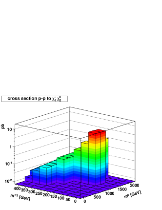
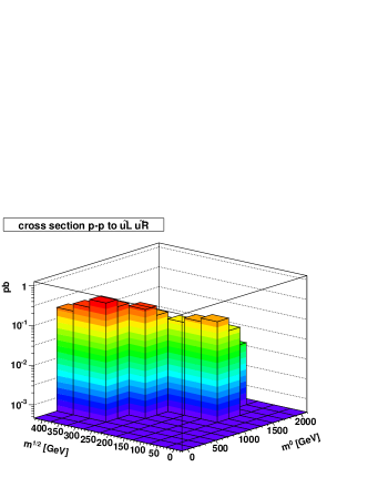
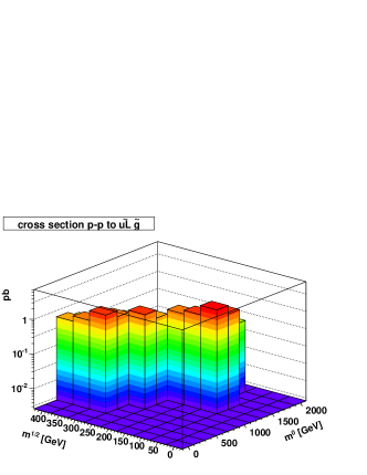
Figure 19: The cross sections of superpartners creation as functions of $m_{1/2}$ and $m_{0}$ for $\tan\beta=51$, $A_{0}=0$ and positive sign of $\mu$.

In most of the cases the superpartners are very short lived and decay practically at the collision point without leaving a secondary vertex. One then has hadron jets (mostly b-jets) and leptons flying outside. The typical process of gluino production is presented in Fig.20 where the cascade decay of one of the gluinos is shown [50]. For a given choice of soft SUSY breaking parameters the cross-section at the first stage reaches 13 pb but with the 4-lepton + 4-jet final state is reduced to a few fb. To distinguish this reaction from the background one has to perform the analysis of the missing energy and consider the peculiarities in the invariant mass distribution of the muon pair, free pass of B-mesons, etc [50].

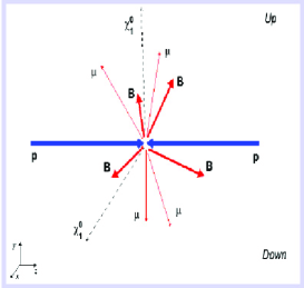
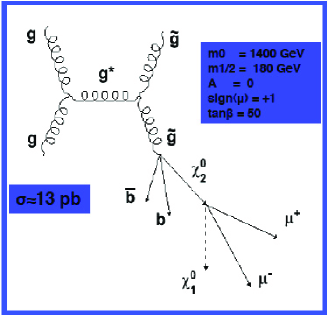
Figure 20: Gluino production at the LHC accompanied with cascade decays

6.6 The long-lived superpartners

Within the framework of Constrained MSSM with gravity mediated soft supersymmetry breaking mechanism there exists an interesting possibility to get long-lived next-to-lightest supersymmetric particles (staus or stops or charginos). Their production cross-sections crucially depend on a single parameter, the mass of the superparticle, and for light staus can reach a few % of pb. This might be within the LHC reach. The stop production cross-section can achieve even hundreds pb. Decays of long-lived superpartners would have an unusual signature if heavy charged particles decay with a considerable delay producing secondary vertices inside the detector, or even escape the detector. This possibility can be realized at the boundary regions of allowed parameter space where one can have a mass degeneracy between the LSP and the NLSP. The life time of the NLSP is inversely proportional to the mass degeneracy.

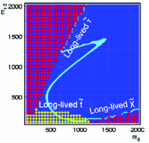
Figure 21: The regions of the parameters space of mSUGRA where the long-lived sparticles might exist

We show in Fig.21 the regions where this might happen. The first region is the so-called co-annihilation region which is interesting from the point of view of existence of long-lived charged sleptons. Their life-time may be large enough to be produced in proton-proton collisions and to fly away from the detector area or to decay inside the detector at a considerable distance from the collision point. Clearly that such an event can not be unnoticed. However, to realize this possibility one need a fine-tuning of parameters of the model [51]. The second region is the border of the bulk region where light long-lived stops can exist. It appears only for large negative trilinear soft supersymmetry breaking parameter $A_{0}$. On the border of this region, in full analogy with the stau co-annihilation region, the top squark becomes the LSP and near this border one might get the long-lived stops. Stops can form the so-called R-hadrons (bound states of SUSY particles) if their lifetime is bigger than the hadronisation time.

The last interesting region of parameter space is a narrow band along the line where the radiative electroweak symmetry breaking fails. On the border of this region the Higgs mixing parameter $\mu$, which is determined from the requirement of electroweak symmetry breaking via radiative corrections, tends to zero. This leads to existence of light and degenerate states: the second chargino and two neutralinos, all of them being essentially higgsinos.

Experimental Higgs and chargino mass limits as well as WMAP relic density limit can be easily satisfied in these scenarios. However, the strong fine-tuning is required. The discussed scenarios differ from the GMSB scenario [52] with the gravitino as the LSP, and next-to-lightest supersymmetric particles typically live longer.

Searches for long-lived particles were already made by LEP collaborations [53]. It is also of great interest at the moment since the first physics results of the coming LHC are expected in the nearest future. Light long-lived sparticles could be produced already during first months of its operation [54]. Since staus and stops are relatively light in this scenario, their production cross-sections are quite large and may achieve a few per cent of pb for stau production, and tens or even hundreds of pb for light stops, $\tilde{m}_{t}<150$ GeV. The cross-section then quickly falls down when the mass of stop is increased. However, even for very large values of $|A|$ when stops become heavier than several hundreds GeV, the production cross-section is of order of few per cent of pb, which is enough for detection with the high LHC luminosity.

6.7 The reach of the LHC

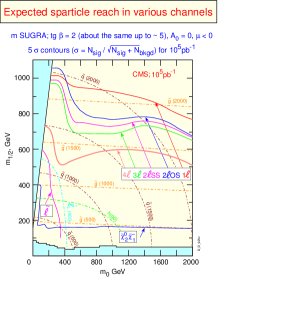
Figure 22: Expected range of reach for superpartners in various channels at LHC [55].

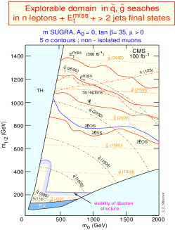
Figure 23: Expected domain of searches for squarks and gluions at LHC [55].

The LHC hadron collider is the ultimate machine for new physics at the TeV scale. Its c.m. energy is planned to be 14 TeV with very high luminosity up to a few hundred fb^-1. The LHC is supposed to cover a wide range of parameters of the MSSM (see Figs. below) and discover the superpartners with the masses below 2 TeV [56]. This will be a crucial test for the MSSM and the low energy supersymmetry. The LHC potential to discover supersymmetry is widely discussed in the literature [56]-[57].

To present the region of reach for the LHC in different channels of sparticle production it is useful to take the same plane of soft SUSY breaking parameters $m_{0}$ and $m_{1/2}$. In this case one usually assumes certain luminosity which will be presumably achieved during the accelerator operation.

Thus, for instance, in Fig. 22 it is shown the regions of reach in different channels. The lines of a constant squark mass form the arch curves, and those for gluino are almost horisontal. The curved lines show the reach bounds in different channel of creation of secondary particles. The theoretical curves are obtained within the MSSM for a certain choice of the other soft SUSY breaking parameters. As one can see, for the fortunate circumstances the wide range of the parameter space up to the masses of the order of 2 Tev will be examined.

The other example is shown in Fig. 23 where the regions of reach for squarks and gluino are shown for various luminosities. One can see that for the maximal luminosity the discovery range for squarks and gluino reaches 3 TeV for the center of mass energy of 14 TeV and even higher for the double energy.

The LHC will be able to discover SUSY with squark and gluino masses up to $2\div 2.5$ TeV for the luminosity $L_{tot}=100\ fb^{-1}$. The most powerful signature for squark and gluino detection are multijet events; however, the discovery potential depends on relation between the LSP, squark, and gluino masses, and decreases with the increase of the LSP mass.

The same is true for the sleptons as shown in Fig. 24. The slepton pairs can be created via the Drell-Yang mechanism $pp\to\gamma^{*}/Z^{*}\to\tilde{\ell}^{+}\tilde{\ell}^{-}$ and can be detected through the lepton decays $\tilde{\ell}\to\ell+\tilde{\chi}^{0}_{1}$. The typical signal used for slepton detection is the dilepton pair with the missing energy without hadron jets. For the luminosity of $L_{tot}=100$ fb^-1 the LHC will be able to discover sleptons with the masses up to 400 GeV [56]. The discovery reach for sleptons in various channels is shown in Fig.24.

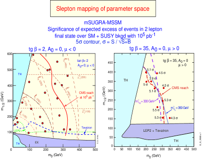
Figure 24: Expected range of reach for sleptons at LHC [55].

6.8 The lightest superparticle

One of the crucial questions is the properties of the lightest superparticle. Different SUSY breaking scenarios lead to different experimental signatures and different LSP.

$\bullet$ Gravity mediation

In this case, the LSP is the lightest neutralino $\tilde{\chi}^{0}_{1}$, which is almost 90% photino for a low $\tan\beta$ solution and contains more higgsino admixture for high $\tan\beta$. The usual signature for LSP is missing energy; $\tilde{\chi}^{0}_{1}$ is stable and is the best candidate for the cold dark matter in the Universe. Typical processes, where the LSP is created, end up with jets + $\Big{/}E_{T}$, or leptons + $\Big{/}E_{T}$, or both jets + leptons + $/E_{T}$.

$\bullet$ Gauge mediation

In this case the LSP is the gravitino $\tilde{G}$ which also leads to missing energy. The actual question here is what the NLSP, the next lightest particle, is. There are two possibilities:

i) $\tilde{\chi}^{0}_{1}$ is the NLSP. Then the decay modes are:  $\tilde{\chi}^{0}_{1}\to\gamma\tilde{G},\ h\tilde{G},\ Z\tilde{G}.$ As a result, one has two hard photons + $/E_{T}$, or jets + $/E_{T}$.

ii) $\tilde{l}_{R}$ is the NLSP. Then the decay mode is $\tilde{l}_{R}\to\tau\tilde{G}$ and the signature is a charged lepton and the missing energy.

$\bullet$ Anomaly mediation

In this case, one also has two possibilities:

i) $\tilde{\chi}^{0}_{1}$ is the LSP and wino-like. It is almost degenerate with the NLSP.

ii) $\tilde{\nu}_{L}$ is the LSP. Then it appears in the decay of chargino $\tilde{\chi}^{+}\to\tilde{\nu}l$ and the signature is the charged lepton and the missing energy.

$\bullet$ R-parity violation

In this case, the LSP is no longer stable and decays into the SM particles. It may be charged (or even colored) and may lead to rare decays like neutrinoless double $\beta$-decay, etc.

Experimental limits on the LSP mass follow from non-observation of the corresponding events. Modern lower limit is around 40 GeV .

7 Supersymmetric Dark Matter

7.1 The problem of the dark matter in the Universe

As was already mentioned the shining matter does not compose all the matter in the Universe. According to the latest precise data [58] the matter content of the Universe is the following:

$$\Omega_{total}=1.02\pm 0.02,$$

$$\Omega_{vacuum}=0.73\pm 0.04,$$

$$\Omega_{matter}=0.23\pm 0.04,$$

$$\Omega_{baryon}=0.044\pm 0.004,$$

so that the dark matter prevails the usual matter by factor of 6.

Besides the rotation curves of stars the dark matter manifests itself in the observation of gravitational lensing effects [59] and the large structure formation. It is believed that the dark matter played the crucial role in formation of large structures like clusters of galaxies and the usual matter just fell down in a potential well attracted by gravitational interaction afterwards. The dark matter can not make compact objects like the usual matter since it does not take part in strong interaction and can not lose energy by photon emission since it is neutral. For this reason the dark matter can be trapped in much larger scale structures like galaxies.

In general one may assume two possibilities: either the dark matter interacts only gravitationally, or it participates also in the weak interaction. The latter case is preferable since then one may hope to detect it via the methods of particle physics. What makes us to believe that the dark matter is probably the Weakly Interacting Massive Particle (WIMP)? This is because the cross-section of DM annihilation which can be figured out of the amount of the DM in the Universe is close to a typical weak interaction cross-section. Indeed, let us assume that all the DM is made of particles of a single type. Then the amount of the DM can be calculated from the Boltzman equatio [60, 61]

$$\frac{dn_{\chi}}{dt}+3Hn_{\chi}=-<\sigma v>(n^{2}_{\chi}-n^{2}_{\chi,eq}),$$ (7.1)

where $H=\dot{R}/R$ is the Hubble constant and $n_{\chi,eq}$ is the equilibrium concentration. The relic abundance is expressed in terms of $n_{\chi}$ as

$$\Omega_{\chi}h^{2}=\frac{m_{\chi}n_{\chi}}{\rho_{c}}\approx\frac{2\cdot 10^{27}\ cm^{3}\ sec^{-1}}{<\sigma v>}.$$ (7.2)

Having in mind that $\Omega_{\chi}h^{2}\approx 0.113\pm 0.009$ and $v\sim 300$ km/sec one gets

$$\sigma\approx 10^{-34}\ cm^{2}=100\ pb,$$ (7.3)

which is a typical EW cross-section.

7.2 Detection of the Dark matter

There are two methods of the DM detection: direct and indirect. In direct detection one assumes that the particles of DM come to Earth and interact with the nuclei of a target. In underground experiments one can hope to observe such events measuring the recoil energy. There are several experiments of this type: DAMA, Zeplin, CDMS and Edelweiss. Among them only DAMA collaboration claims to observe a positive outcome in annual modulation of the signal with the fitted DM particle mass around 50 GeV [62].

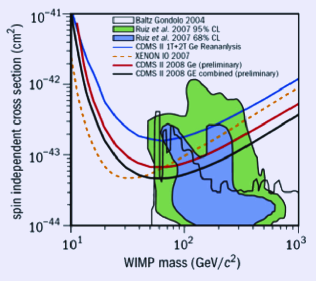
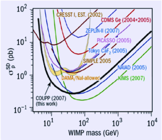
Figure 25: The exclusion plots from direct DM detection experiments. Spin-independent case (top) from Chicagoland Observatory for Underground Particle Physics (COUPP) and spind-dependent case (bottom) from Cryogenic Dark Matter Search (CDMS)

All the other experiments do not see it though CDMS collaboration recently announced about a few events of a desired type [63]. The reason of this disagreement might be in different methodology and the targets used since the cross-section depends on a spin of a target nucleus. The collected statistics is also essentially different, DAMA has accumulated by far more data and this is the only collaboration which studies the modulation of the signal that may be crucial for reducing the background.

The typical exclusion plots for spin-independent and spin-dependent cross-sections are shown in Fig.25 where one can see DAMA allowed region overlapping with the other exclusion ones. Still today we have no convincing evidence for direct DM detection or exclusion.

Indirect detection of the DM is aimed to the registration of a signal from the DM annihilation in the form of additional gamma rays and charged particles (antiprotons and positrons) in cosmic rays. These particles should have the energetic spectrum reflecting their origin from annihilation of heavy massive particles which is different from the background coming from the known sources. Hence one may expect the appearance of a ”shoulder“ in the cosmic ray spectrum. There are several experiments of this kind: EGRET (diffuse gamma rays) which is followed by FERMI; HEAT and AMS1 (positrons) which is followed by PAMELA; BESS (antiprotons) which will be followed by PAMELA and AMS2. All these experiments see some deviation from the background though the uncertainties are large and the background is not known very accurately especially for charged particles.

From this point of view the most detailed information was obtained by EGRET cosmic telescope [64] which orbited the Earth for 9 years and measured the spectrum and intensity of diffuse gamma rays over the whole celestial sphere with the 4 degree bins. The form of the spectrum was measured in the region of 0.1-10 GeV. It allows one to perform the independent analysis in different directions of the celestial sphere. Gamma rays have the advantage that they point back to the source and do not suffer energy losses, so they are the ideal candidates to trace the dark matter density. The charged components interact with Galactic matter and are deflected by the Galactic magnetic field, so they do not point back to the source.

The diffuse component shows a clear excess for the energy above 1 GeV about a factor two over the expected background from known nuclear interactions, inverse Compton scattering and bremsstrahlung as shown in Fig.27 [65]. Different plots correspond to different regions in the sky: A - inner galaxy, B - outer disk, C - outer galaxy, D- low attitude, E- intermediate latitude, F -galactic poles.

As one can see the excess of a signal above the background is isotropic in celestial sphere that suggests the common source which might be the DM. It was shown that the observed excess in the spectrum of diffuse gamma reays, if taken seriously, has all the features of the decay of $\pi^{0}$ mesons produced by monoenergetic quarks coming from the DM annihilation. Fitting the background together with the signal from the DM annihilation one can get remarkable agreement for all directions if the mass of the DM particle is around 60 GeV. A detailed picture for the region of the sky in the direction of the galactic center is shown in Fig.28. Here one can see the allowed background variations and the variations of the DM particle mass used for fitting the data. Possible background variations are not enough to ex-

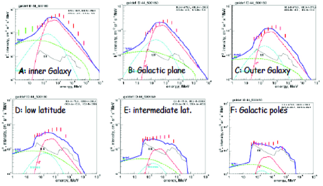
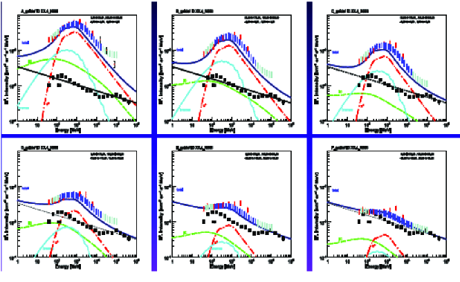
Figure 26: Excess in diffuse gamma rays as measured by EGRET in various regions in the sky. The solid(blue) line is the background as calculated by the GALPROP code. Discrete slashes represent EGRET data. Also shown are the contributions of the known background sources

Figure 27: Excess in diffuse gamma rays as measured by FERMI - dark (blue) slashes in comparison with EGRET - light (red) slashes in the same regions in the sky

plain EGRET data while the variation of the WIMP mass within 50-70 GeV does not contradict these data.

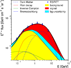
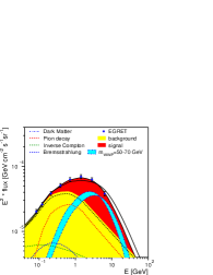
Figure 28: The spectrum of diffuse gamma rays measured by EGRET in the direction of the galaxy center and the fit to the data. The light shaded (yellow) areas indicate the background using the shape of the conventional GALPROP model [66], while the dark shaded (red) areas are the signal contribution from DMA for a 60 GeV WIMP mass.

It is instructive to compare EGRET data with recently released FERMI data which are much more precise. This comparison is shown in Fi.27 [67]. One can see that the new data are not in contradiction with the old ones. The excess is still visible though is smaller compared to EGRET. On has to admit, however, that the interpretation of the data in favour of background modification is also possible. So, taking the optimistic point of view, one can interpret these data as a signal from the DM annihilation, otherwise everything is sinked in the error bars.

The experimental data with the charge particles looks more contradictory. We present the antiproton and positron data in Figs. 29 [68] and 30 [69], respectively. While there is no excess observed in antiproton data, the positron spectrum measured by PAMELA is quite unusual. It strongly contradicts the expectations from the GALPROP. Possible interpretations of PAMELA data include: background from hadronic showers with large electromagnetic component; astrophysical sources like pulsars, positron acceleration in SNR, locality of sources; leptophilic DM annihilation, very heavy ($\sim$ 1 TeV) WIMPs, etc. The situation is still to be clarified.

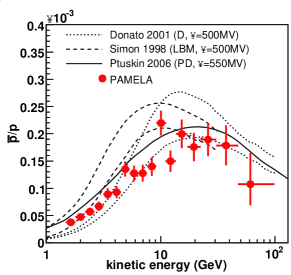
Figure 29: Antiproton/proton ratio as measured by PAMELA. No excess is found

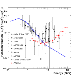
Figure 30: Positron fraction as measured by PAMELA in comparison with the background

One should mention here, that interpreting the excess in diffuse gamma rays data as the WIMP annihilation one has to enhance the intensity of a signal by factor of 10-100 that is usually achieved by assumption of clumpiness of the DM. This almost obvious property of the DM has no experimental confirmation so far. The same enhancement, however, is not needed for antiprotons where one seems to have an agreement with the data. This contradiction might be attributed to different behaviour of charged particles in galactic magnetic fields.

7.3 Supersymmetric Interpretation of the Dark Matter

Supersymmetry offers several candidates for the role of the cold dark matter. If one looks at the particle content of the MSSM from the point of view of a heavy neutral particle, one finds several such particles, namely: a superpartner of the photon (photino $\tilde{\gamma}$), a superpartner of the Z-boson (zino $\tilde{z}$), a superpartner of neutrino (sneutrino $\tilde{\nu}$) and superpartners of the Higgs bosons (higgsino $\tilde{H}$). The DM particle can be the lightest of them, the LSP. The others decay on the LSP and the SM particles, while the LSP is stable and can survive since the Big Bang. As a rule the lightest supersymmetric particle is the so-called neutralino, the spin 1/2 particle which is the combination of photino, zino and two neutral higgsinos and is the eigenstate of the mass matrix

$$|\tilde{\chi}^{0}_{1}\rangle=N_{1}|B_{0}\rangle+N_{2}|W^{3}_{0}\rangle+N_{3}|H_{1}\rangle+N_{4}|H_{2}\rangle.$$

Thus, supersymmetry actually predicts the existence of the dark matter. Moreover, we have shown above that one can choose the parameters of a soft supersymmetry breaking in such a way that one gets the right amount of the DM. This requirement serves as a constraint for these parameters and is consistent with the requirements coming from particle physics.

The search for the LSP was one of the tasks of LEP. They were supposed to be produced as a result of chargino decays and be detected via missing transverse energy and momentum. Negative results defined the limit on the LSP mass as shown in Fig.31.

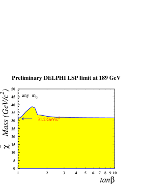
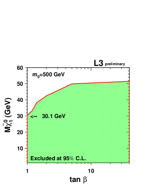
Figure 31: Exclusion limit on the LSP mass from Delphi coll. and L3 coll. (LEP) [70]

The DM particles which form the halo of the galaxy annihilate to produce the ordinary particles in the cosmic rays. Identifying them with the LSP from a supersymmetric model one can calculate the annihilation rate and to study the secondary particle spectrum. The dominant annihilation diagrams of the lightest supersymmetric particle (LSP) neutralino are shown in Fig.32. The usual final states are either the quark-antiquark pairs or the W and Z bosons. Since the cross sections are proportional to the final state fermion mass, the heavy fermion final states, i.e. third generation quarks and leptons, are expected to be dominant. The W- and Z-final states from t-channel chargino and neutralino exchange have usually a smaller cross section.

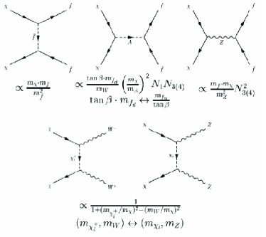
Figure 32: The dominant annihilation diagrams for the lightest neutralino in the MSSM

The dominant contribution comes from A-boson exchange: $\chi+\chi\to A\to b\bar{b}$. The sum of the diagrams should yield $<\sigma v>=2\cdot 10^{-26}\ cm^{3}/sec$ to get the correct relic density.

The spectral shape of the secondary particles from DMA is well known from the fragmentation of mono-energetic quarks studied at electron-positron colliders, like LEP at CERN, which has been operating up to centre-of-mass energies of about 200 GeV, i.e. it corresponds to the neutralino masses up to 100 GeV (see Fig.33). The different quark flavours all yield similar gamma spectra at high energies. Hence, the specrta of positrons, gammas and antiprotons is known. The relative ammount of $\gamma,p^{-}$ and $e^{+}$ is also known. One expects around 37 gammas per collision.

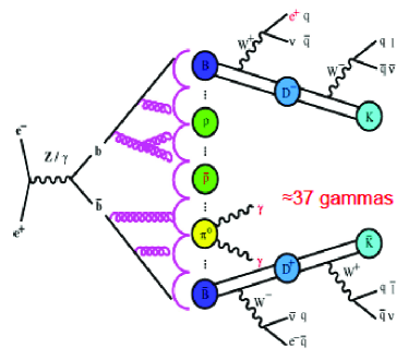
Figure 33: The final states in the process of $e^{+}e^{-}$-annihilation at colliders in the SM

The gamma rays from the DM annihilation can be distinguished from the background by their completely different spectral shape: the background originates mainly from cosmic rays hitting the gas of the disc and producing abundantly $\pi^{0}$ mesons, which decay into two photons. The initial cosmic ray spectrum is a steep power law spectrum, which yields a much softer gamma ray spectrum than the fragmentation of the hard mono-energetic quarks from the DM annihilation. The spectral shape of the gamma rays from the background is well known from fixed target experiments given the known cosmic ray spectrum.

7.4 SUSY interpretation of EGRET excess

If one takes the EGRET excess in diffuse gamma rays seriously then one can try to identify the DM particle responsible for this excess with the LSP. The mass of this hypothetical WIMP as it follows from EGRET data is in the range of 50 to 100 GeV and is fully compatible with the neutralino. Since in the MSSM all the couplings are known one can calculate the annihilation rate given by the diagrams in Fig.32. The only unknown parameters are the SUSY masses (and mixings) which one can choose to fit the data.

Combining various requirements on soft SUSY parameters together with the assumed EGRET energy range for the mass of neutralino one gets an essentially constrained allowed region shown in Fig.34 [71]

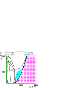
Figure 34: The allowed region of parameter space with account of the EGRET data on diffuse gamma rays. The star indicates the best fir value.

One can see that the ”EGRET” region of parameter space corresponds to high values of $\tan\beta$, low $m_{1}/2$ and high $m_{0}$. This is the range of the so-called focus point region where chrarginos and neutralinos, whose mass is governed by the value of $m_{1}/2$, are light and squarks and sleptons, whose mass is governed by $m_{0}$, are heavy. The lightest neutralino in the this region is 95% photino being the superpartner of a photon of the cosmic microwave background. Choosing the point in this allowed region one can calculate the whole mass spectrum of superpartners. We present in the Table5 the sample mass spectrum corresponding to the best fit point in the ”EGRET” region. [71].

Particle	Mass [GeV]
$\tilde{\chi}^{0}_{1,2,3,4}$	64, 113, 194, 229
$\tilde{\chi}^{\pm}_{1,2},\tilde{g}$	110, 230, 516
$\tilde{u}_{1,2}=\tilde{c}_{1,2}$	1519, 1523
$\tilde{d}_{1,2}=\tilde{s}_{1,2}$	1522, 1524
$\tilde{t}_{1,2}$	906, 1046
$\tilde{b}_{1,2}$	1039, 1152
$\tilde{e}_{1,2}=\tilde{\mu}_{1,2}$	1497, 1499
$\tilde{\tau}_{1,2}$	1035, 1288
$\tilde{\nu}_{e},\tilde{\nu}_{\mu},\tilde{\nu}_{\tau}$	1495, 1495, 1286
$h,H,A,H^{\pm}$	115, 372, 372, 383
Observable	Value
$Br(b\to s\gamma)$	$3.02\cdot 10^{-4}$
$\Delta a_{\mu}$	$1.07\cdot 10^{-9}$
$\Omega h^{2}$	$0.117$

Table 5: The mass spectrum of superpartners in the EGRET point: $m_{0}=1500$ , $m_{1/2}=170$ , $A_{0}=0$, $\tan\beta=52.2$, $\mu>0$

As one can see from the table, in the ”EGRET” point one has considerable splitting between the relatively light superpartners of the gauge fields and heavy squarks and sleptons. The masses of neutralinos and charginos are almost at the lower boundary of experimentally allowed range. The same is true for the lightest Higgs boson. Experimental lower limit on the SM Higgs boson mass today is 114.7 GeV as follows from the negative results of the search at LEP. This bound is also true for the MSSM for large $\tan\beta$.

Thus, taking the optimistic point of view that the excess in diffuse gamma rays actually exists and accepting the supersymmetric interpretation of this excess one can simultaneously give answer to the following questions:
$\bullet$ In Cosmology: What is CDM made of?
$\bullet$ In Astrophysicists: What is the origin of excess of diffuse Galactic Gamma Rays?
$\bullet$ In Particle physicists : Where are the Supersymmetric Particles?
And the answer is:
$\bullet$ DM is made of WIMPs which are SUSY particles distributed in Halo of our Galaxy with a mass around 70 GeV.

What is important, supersymmetric interpretation of the DM is testable since it predicts the mass spectrum which can be directly checked at the LHC in the nearest future.

8 Conclusion

Supersymmetry is now the most popular extension of the Standard Model. Comparison of the MSSM with precision experimental data for the MSSM is as good as for the SM and sometimes even better. For example the branching ratio $BR(b\to s\gamma)$ and the anomalous magnetic moment of muon are fitted better in the MSSM than in the SM. The relic density of the DM is not described in the SM but is naturally predicted by the MSSM. One can see this comparison for main observables in Fig.35 [45].

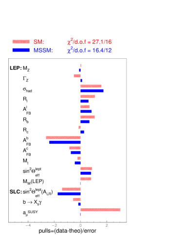
Figure 35: The SM versus the MSSM in comparison with precision experimental data

Still today after 30 years since the invention of supersymmetry we have no single convincing evidence that supersymmetry is realized in particle physics. It remains very popular in quantum field theory and in string theory due to its exceptional properties but needs experimental justification.

Let us remind the main pros and contras for supersymmetry in particle physics

Pro:
$\bullet$ Provides natural framework for unification with gravity
$\bullet$ Leads to gauge coupling unification (GUT)
$\bullet$ Solves the hierarchy problem
$\bullet$ Is a solid quantum field theory
$\bullet$ Provides natural candidate for the WIMP cold DM
$\bullet$ Predicts new particles and thus generates new job positions

Contra:
$\bullet$ Does not shed new light on the problem of

$*$ Quark and lepton mass spectrum

$*$ Quark and lepton mixing angles

$*$ the origin of CP violation

$*$ Number of flavours

$*$ Baryon assymetry of the Universe
$\bullet$ Doubles the number of particles

Low energy supersymmetry promises us that new physics is round the corner at a TeV scale to be exploited at colliders and astroparticle experiments of this decade. If our expectations are correct, very soon we will face new discoveries, the whole world of supersymmetric particles will show up and the table of fundamental particles will be enlarged in increasing rate. This would be a great step in understanding the microworld. The future will show whether we are right in our expectations or not.

Acknowledgements

The author would like to express his gratitude to the organizers of the School for their effort in creating a pleasant atmosphere and support. This work was partly supported by RFBR grant # 08-02-00856 and Russian MIST grant # 1027.2008.2. I would also like to thank A.Gladyshev for his help in preparation of the manuscript.

References

- [1] Y. A. Golfand and E. P. Likhtman, JETP Letters 13 (1971) 452; D. V. Volkov and V. P. Akulov, JETP Letters 16 (1972) 621; J. Wess and B. Zumino, Phys. Lett. B49 (1974) 52.
- [2] P. Fayet and S. Ferrara, Phys. Rep. 32 (1977) 249; M. F. Sohnius, Phys. Rep. 128 (1985) 41; H. P. Nilles, Phys. Rep. 110 (1984) 1; H. E. Haber and G. L. Kane, Phys. Rep. 117 (1985) 75; A. B. Lahanas and D. V. Nanopoulos, Phys. Rep. 145 (1987) 1.
- [3] J. Wess and J. Bagger, ”Supersymmetry and Supergravity”, Princeton Univ. Press, 1983.
- [4] A. Salam, J. Strathdee, Nucl. Phys. B76 (1974) 477; S. Ferrara, J. Wess, B. Zumino, Phys. Lett. BS1 (1974) 239.
-
[5]
S. J. Gates, M. Grisaru, M. Roček and W. Siegel,
”Superspace or One Thousand and One Lessons in
Supersymmetry”, Benjamin & Cummings, 1983;
P. West, ”Introduction to supersymmetry and supergravity”, World Scientific, 2nd ed., 1990.
S. Weinberg,”The quantum theory of fields”. Vol. 3, Cambridge, UK: Univ. Press, 2000. - [6] S. Coleman and J .Mandula, Phys.Rev. 159 (1967) 1251.
- [7] G. G. Ross, ”Grand Unified Theories”, Benjamin & Cummings, 1985.
- [8] C. Amsler et al. (Particle Data Group), Phys. Lett. B667 (2008) 1.
- [9] U. Amaldi, W. de Boer and H. Fürstenau, Phys. Lett. B260 (1991) 447.
- [10] Y. Sofue, V. Rubin, Rotation curves of spiral galaxies, Ann. Rev. Astron. Astrophys. 39 (2001) 137, astro-ph/0010594, and refs therein.
- [11] V.A. Ryabov, V.A. Tsarev and A.M. Tskhovrebov, The search for dark matter particles, Phys. Usp. 51 (2008) 1091, and refs therein.
-
[12]
G.Jungman, M.Kamionkowski and K.Griest, Phys.Rep.
267 (1996) 195;
H. Goldberg, Phys. Rev. Lett. 50 (1983) 1419;
J.R. Ellis, J.S. Hagelin, D.V. Nanopoulos, K.A. Olive, M. Srednicki, Nucl. Phys. B238 (1984) 453. - [13] M. B. Green, J. H. Schwarz and E. Witten, ”Superstring Theory”, Cambridge, UK: Univ. Press, 1987. Cambridge Monographs On Mathematical Physics.
- [14] M. Peskin and D. Schreder, ”An Introduction to Quantum Field Theory”, Addison-Wesley Pub. Company, 1995
- [15] H.Baer and X.Tata, ”Weak Scale Supersymmetry”, Cambridge University Press, 2006.
-
[16]
H. E. Haber, ”Introductory Low-Energy Supersymmetry”,
Lectures given at TASI 1992, (SCIPP 92/33, 1993),
hep-ph/9306207.
D. I. Kazakov, ”Beyond the Standard Model (In search of supersymmetry)”, Lectures at the European school on high energy physics, CERN-2001-003, hep-ph/0012288.
D. I. Kazakov, Beyond the Standard Model, Lectures at the European school on high energy physics 2004, hep-ph/0411064;
A.V. Gladyshev, D.I. Kazakov, Supersymmetry and LHC, Phys. Atom. Nucl. 70 (2007) 1553-1567, hep-ph/0606288. - [17] http://atlasinfo.cern.ch/Atlas/documentation /EDUC/physics14.html
- [18] F. A. Berezin, ”The Method of Second Quantization”, Moscow, Nauka, 1965.
- [19] P.Fayet, Nucl. Phys. B90(1975) 104; A.Salam and J.Srathdee, Nucl. Phys. B87(1975) 85.
- [20] P. Fayet and J. Illiopoulos, Phys. Lett. B51 (1974) 461.
- [21] L.O’Raifeartaigh, Nucl.Phys. B96 (1975) 331
- [22] L. Hall, J. Lykken and S. Weinberg, Phys. Rev. D27 (1983) 2359; S. K. Soni and H. A. Weldon, Phys. Lett. B126 (1983) 215; I. Affleck, M. Dine and N. Seiberg, Nucl. Phys. B256 (1985) 557.
- [23] H. P. Nilles, Phys. Lett. B115 (1982) 193; A. H. Chamseddine, R. Arnowitt and P. Nath, Phys. Rev. Lett. 49 (1982) 970; Nucl. Phys. B227 (1983) 121; R. Barbieri, S. Ferrara and C. A. Savoy, Phys. Lett. B119 (1982) 343.
- [24] M. Dine and A. E. Nelson, Phys. Rev. D48 (1993) 1277, M. Dine, A. E. Nelson and Y. Shirman, Phys. Rev. D51 (1995) 1362.
- [25] L. Randall and R. Sundrum, Nucl. Phys. B557 (1999) 79; G. F. Giudice, M. A. Luty, H. Murayama and R. Rattazzi, JHEP, 9812 (1998) 027.
- [26] D. E. Kaplan, G. D. Kribs and M. Schmaltz, Phys. Rev. D62 (2000) 035010; Z. Chacko, M. A. Luty, A. E. Nelson and E. Ponton, JHEP, 0001 (2000) 003.
-
[27]
G. G. Ross and R. G. Roberts, Nucl. Phys. B377 (1992) 571.
V. Barger, M. S. Berger and P. Ohmann, Phys. Rev. D47 (1993) 1093. -
[28]
W. de Boer, R. Ehret and D. Kazakov, Z. Phys.
C67 (1995) 647;
W. de Boer et al., Z. Phys. C71 (1996) 415. - [29] L. E. Ibáñez, C. Lopéz and C. Muñoz, Nucl. Phys. B256 (1985) 218.
- [30] W. Barger, M. Berger, P. Ohman, Phys. Rev. D49 (1994) 4908.
-
[31]
V.Barger, M.S. Berger, P.Ohmann and R.Phillips,
Phys. Lett. B314 (1993) 351.
P. Langacker and N. Polonsky, Phys. Rev. D49 (1994) 1454.
S. Kelley, J. L. Lopez and D.V. Nanopoulos, Phys. Lett. B274 (1992) 387. -
[32]
M. Carena, M. Quiros and C. E. M. Wagner,
Nucl. Phys. B461 (1996) 407;
A.V. Gladyshev, D.I. Kazakov, W. de Boer, G. Burkart, R. Ehret, Nucl. Phys. B498 (1997) 3; A.V. Gladyshev, D.I. Kazakov, Mod. Phys. Lett. A10 (1995) 3129. - [33] S. Heinemeyer, W. Hollik and G. Weiglein, Phys. Lett. B455 (1999) 179; Eur. Phys. J. C9 (1999) 343.
- [34] S.Ahmed et al. (CLEO Collab.), CLEO CONF 99/10, hep-ex/9908022.
- [35] R. Barate et al. (ALEPH Collab.), Phys. Lett. B429 (1998) 169.
- [36] CDF Collab., F. Abe et al., Phys. Rev. D 57, (1998) 3811.
- [37] ALEPH Collab., Phys.Lett. B499 (2001) 67.
- [38] S. Abel et al. [SUGRA Working Group Collaboration], Report of the SUGRA working group for run II of the Tevatron, hep-ph/0003154.
-
[39]
M. Drees and M. M. Nojiri, Phys. Rev. D47
(1993) 376;
J. L. Lopez, D. V. Nanopoulos and H. Pois, Phys. Rev. D47 (1993) 2468;
P. Nath and R. Arnowitt, Phys. Rev. Lett. 70 (1993) 3696. -
[40]
W.de Boer, H.J.Grimm, A.Gladyshev, D.Kazakov, Phys. Lett. B438 (1998) 281;
W.de Boer, M.Huber, A.Gladyshev, D.Kazakov, Eur.Phys.J. C20 (2001) 689;
W.de Boer, M.Huber, A.Gladyshev, D.Kazakov, The decay rate in NLO, Higgs boson limits, and LSP masses in the Constrained Minimal Supersymmetric Model, hep-ph/0007078; and refs therein - [41] R. L. Arnowitt, B. Dutta, T. Kamon, and M. Tanaka, Phys.Lett. B538 (2002) 121, e-Print: hep-ph/0203069
- [42] G.W. Bennet et al. [Muon g-2 Collaboration], Phys.Rev.Lett. 92, 161802 (2004);
- [43] A. Czarnecki and W. Marciano, Phys.Rev. D64 (2001) 013014, hep-ph/0102122.
- [44] W.de Boer, M.Huber, C.Sander, D.I. Kazakov, Phys.Lett. B515 (2001) 283.
- [45] W.de Boer and C.Sander, Phys. Lett. B585 (2004) 276.
-
[46]
J. Ellis, K. Olive, Y. Santoso, V. Spanos, Phys. Lett. B565 (2003) 176;
H. Baer, C. Balazs, A. Belyaev,JHEP 0203 (2002) 042; H. Baer, C. Balazs, JCAP 05 (2003) 006;
A. Lahanas, D. V. Nanopoulos, Phys. Lett. B568 (2003) 55; A. B.Lahanas, N. E. Mavromatos, D. V. Nanopoulos, Int. J. Mod. Phys. D12 (2003) 1529. - [47] W.de Boer, M.Herold, C.Sander, V.Zhukov, A.Gladyshev, and D.Kazakov, Excess of egret galactic gamma ray data interpreted as dark matter annihilation, astro-ph/0408272.
-
[48]
CDF Collaboration (D. Acosta et al.),
Phys.Rev.Lett. 90 (2003) 251801;
CDF Collaboration (T. Affolder et al.), Phys.Rev.Lett. 87 (2003) 251803;
T.Kamon, hep-ex/0301019, Proc. of IX Int. Conf. ”SUSY-01”, WS 2001, p.196. - [49] D. Yu. Bogachev, A. V. Gladyshev, D. I. Kazakov, A. S. Nechaev, Int. J. Mod. Phys. A21 (2006) 5221.
-
[50]
V.A. Bednyakov, J.A. Budagov, A.V. Gladyshev, D.I. Kazakov, E.V. Khramov, D.I. Khubua,
Phys. Part. Nucl. Lett. 5 (2008) 520;
V.A. Bednyakov, J.A. Budagov, A.V. Gladyshev, D.I. Kazakov, E.V. Khramov, D.I. Khubua, Phys. Atom. Nucl. 72 (2009) 619. - [51] A.V. Gladyshev, D.I. Kazakov, M.G. Paucar, Mod. Phys. Lett. A20 (2005) 3085; A.V. Gladyshev, D.I. Kazakov, M.G. Paucar, Light stops in the MSSM parameter space, arXiv:0704.1429; A.V.Gladyshev, D.I.Kazakov, M.G.Paucar, J.Phys. G36 (2009) 125009; Nucl.Phys.Proc.Suppl. 198 (2010) 104.
-
[52]
P.G. Mercadante, J.K. Mizukoshi, H. Yamamoto,
Phys. Rev. D64 (2001) 015005;
S. Ambrosanio, B. Mele, A. Nisati, S. Petrarca, G. Polesello, A. Rimoldi, G. Salvini, CERN-TH-2000-349, arXiv:hep-ph/0012192. -
[53]
DELPHI Collaboration (P. Abreu et al.), Phys. Lett.
B444 (1998) 491;
DELPHI Collaboration (P. Abreu et al.), Phys. Lett. B478 (2000) 65;
OPAL Collaboration (G. Abbiendi et al.), Phys. Lett. B572 (2003) 8. - [54] B.C. Allanach et al., FERMILAB-CONF-06-338-T, SLAC-PUB-11770, arXiv:hep-ph/0602198; A.M. Abazov et al., Phys. Lett. B645 (2007) 119.
- [55] http://CMSinfo.cern.ch/Welcome.html/CMSdocuments/CMSplots
- [56] N.V.Krasnikov and V.A.Matveev, ”Search for new physics at LHC”, Phys.Atom.Nucl. 73 (2010) 191
-
[57]
F.E.Paige, ”SUSY Signatures in ATLAS at LHC”, hep-ph/0307342;
D.P.Roy, ”Higgs and SUSY Searches at LHC:an Overview”, Acta Phys.Polon. B34 (2003) 3417, hep-ph/0303106;
D.R.Tovey, ”Measuring the SUSY Mass Scale at the LHC”, Phys.Lett. B498 (2001) 1;
H.Baer, C.Balaz, A.Belyaev, T.Krupovnickas, and X.Tata, JHEP 0306 (2003) 054;
G.Belanger, F.Boudjema, F.Donato, R.Godbole, and S.Rosier-Lees, ”SUSY Higgs at the LHC: Effects of light charginos and neutralinos”, Nucl.Phys. B581 (2000) 3;
M.Dittmar, ”SUSY discovery strategies at the LHC”, Lectures given at Summer School on Hidden Symmetries and Higgs Phenomena, ZUOZ 16-22 August 1998, hep-ex/9901004. -
[58]
C.L. Bennett et al., Astrophys. J. Suppl. 148 (2003) 1;
D.N. Spergel et al., Astrophys. J. Suppl. 148 (2003) 175. -
[59]
C.S. Kochanek, Astrophys. J. 453 (1995) 545;
N.Kaiser, G.Squires, Astrophys. J. 404 (1993) 441. - [60] E.Kolb and M.S.Turner, The Early Universe, Frontiers in Physics, Addison Wesley, 1990.
- [61] D.S. Gorbunov, V.A. Rubakov, ”Introduction to the theory of the early Universe”, Moscow, URSS, 2008 (in Russian).
- [62] R. Bernabei, et al. (DAMA Coll.), Eur. Phys. J. C56 (2008) 333.
- [63] Z. Ahmed et al. (CDMS Coll.), Science 327 (2010) 1619; Phys. Rev. D81 (2010) 042002.
-
[64]
E. B. Hughes et al., IEEE Trans. Nucl. Sci. NS-27 (1980) 364;
G. Kanbach, Space Sci. Rev. 49 (1988) 69; D. J. Thompson et al., Astrophys. J. S. 86 (1993) 629; D. L. Bertsch et al., Astrophys. J. 416 (1993) 587;
R. C. Hartman et al., (EGRET Collaboration), Astrophys. J. Suppl. 123 (1999) 79;
EGRET public data archive, ftp://cossc.gsfc.nasa.gov/compton/data/egret/. - [65] W. de Boer, C. Sander, V. Zhukov, A. V. Gladyshev, D. I. Kazakov, Astronomy & Astrophysics, 444 (2005) 51.
-
[66]
http://galprop.stanford.edu/web_galprop/
galprop_home/html - [67] W. de Boer, Indirect DM Searches in the Light of ATIC, FERMI, EGRET, and PAMELA, talk at UCLA DM Symp., 2010.
- [68] O.Adriani et al (PAMELA Collab), Phys. Rev.Lett. 102 (2009) 051101, arxive 0810.4994
- [69] O.Adriani et al (PAMELA Collab), Nature 458 (2009) 607, arxive 0810.4995
-
[70]
Delphi Collab., Eur.Phys.J. C1 (1998) 1;
L3 Collab., Phys. Lett. B 472 (2000) 420; - [71] W. de Boer, C. Sander, V. Zhukov, A. V. Gladyshev, D. I. Kazakov, Phys. Lett. B636 (2006) 13, e-Print Archive: hep-ph/0511154.