Ionisation Feedback in Star and Cluster Formation Simulations

Abstract

Feedback from photoionisation may dominate on parsec scales in massive star-forming regions. Such feedback may inhibit or enhance the star formation efficiency and sustain or even drive turbulence in the parent molecular cloud. Photoionisation feedback may also provide a mechanism for the rapid expulsion of gas from young clusters’ potentials, often invoked as the main cause of ’infant mortality’. There is currently no agreement, however, with regards to the efficiency of this process and how environment may affect the direction (positive or negative) in which it proceeds. The study of the photoionisation process as part of hydrodynamical simulations is key to understanding these issues, however, due to the computational demand of the problem, crude approximations for the radiation transfer are often employed.

We will briefly review some of the most commonly used approximations and discuss their major drawbacks. We will then present the results of detailed tests carried out using the detailed photoionisation code mocassin and the SPH+ionisation code iVINE code, aimed at understanding the error introduced by the simplified photoionisation algorithms. This is particularly relevant as a number of new codes have recently been developed along those lines.

We will finally propose a new approach that should allow to efficiently and self-consistently treat the photoionisation problem for complex radiation and density fields.

1 Introduction

Ionising radiation from OB stars influences the surrounding interstellar medium (ISM) on parsec scales. As the gas surrounding a high mass star is heated, it expands forming an HII region. The consequence of this expansion is twofold, on the one hand gas is removed from the centre of the potential, preventing further gravitational collapse and perhaps even disrupting the parent molecular cloud. On the other hand gas is swept up and compressed beyond the ionisation front producing high density regions that may be susceptible to gravitation collapse (i.e. the “collect and collapse” model, Elmegreen et al. 1995). Furthermore, pre-existing, marginally gravitationally stable clouds may also be driven to collapse by the advancing ionisation front (i.e. “radiation-driven implosion”, Bertoldi 1989). Finally, ionisation radiation has also been suggested as a driver for small scale turbulence in a cloud (Gritschneder et al. 2009b). Observations (e.g. Deharveng, these proceedings) and theory (e.g. Dale et al. 2005, 2007, Gritschneder et al. 2009b) often present examples for positive and negative feedback, however, the net effect on the global star formation efficiency is still under debate.

From a theoretical point of view, different groups have performed a number of numerical experiments demonstrating that the efficacy and direction of photoionisation feedback are very sensitive to the specific initial conditions, in particular, to the location of the ionising source(s) and to whether the cloud is initially bound or unbound. This suggests that a parameter space study may be necessary to assess what environmental variables may affect the direction in which feedback proceeds. Several authors in these proceedings discuss the results of recent ionisation feedback simulations (see oral contributions by Arthur, Bisbas, Gritschneder and Walch, and poster contributions by Choudhury, Cornwall, Miao, Motoyama, Rodon and Tremblin).

As the field matures and the codes become more sophisticated it becomes important to assess the accuracy and limitations of the methods currently employed. The computational demand of treating the radiation transfer (RT) and photoionisation (PI) problem within a large scale hydrodynamical simulation has led to the development of approximate algorithms that drastically simplify the physics of RT and PI. In this review we will describe some of the most common approximations employed by current RT+PI implementations, highlighting some potentially important shortcomings. We will then present the result of our ongoing efforts to test current implementations against the 3D Monte Carlo code mocassin (Ercolano et al. 2003, 2005, 2008) which includes all the necessary micro physics and solves the ionisation, thermal and statistical equilibrium in detail.

2 Some Common Approximations

The importance of studying the photoionisation process as part of hydrodynamical star formation simulations has long been recognised. Until very recently, however, due to the complexity and the computational demand of the problem, the evolution of ionised gas regions had only been studied in rather idealised systems (e.g. Yorke et al. 1989; Garcia-Segura & Franco 1996), with simulations often lacking resolution and dimensions. The situation in the latest years has been rapidly improving, however, with more sophisticated implementations of ionised radiation both in grid-based codes (e.g. Mellema et al. 2006; Peters et al. 2010) and Smoothed Particle Hydrodynamical (SPH) codes (e.g. Kessel-Deynet & Burkert 2000; Miao et al. 2006; Dale et al. 2007; Gritschneder et al. 2009; Bisbas et al. 2009). Klessen et al. (2009) and Mac Low et al. (2007) present recent reviews of the numerical methods employed.

While the new codes can achieve higher resolutions and can treat more realistic geometries, the treatment of RT and PI is still rather crude in most cases. Even in the current era of parallel computing, an exact solution of the radiative transfer (RT) and photoionisation (PI) problem in three dimensions within SPH calculations is still prohibitive. Some common approximations include the following:

1. Monochromatic radiation field: In order to avoid the burden of frequency resolved RT calculations, monochromatic calculations are often carried out, where all the ionising flux is assumed to be at 13.6 eV (i.e. the H ionisation potential). This approximation is often implicit in the choice of a single value for the gas opacity, and it is of course implicit to Strömgren-type calculations. Implicit or explicit monochromatic fields have the serious drawback that the ionisation and temperature structure of the gas cannot be calculated.

2. Ionisation and thermal balances: Its equations are not solved or simple heating/cooling functions are employed or the temperature is a simple function of an approximate ionisation fraction. When monochromatic fields are employed it is not possible to calculate the necessary terms to solve the balance equations and idealised temperature distributions must be used.

3. On-the-spot (OTS) approximation (no diffuse field): The OTS approximation is described in detail by Osterbrock & Ferland (2006, page 24). In the OTS approximation the diffuse component of the radiation field is ignored under the assumption that any ionising photon emitted by the gas will be reabsorbed elsewhere, close to where it was emitted, hence not contributing to the net ionisation of the nebula. This is not a bad approximation in the case of reasonably dense homogeneous or smoothly varying density fields, but it is certain to fail in the highly inhomogeneous star-forming gas, where the ionisation and temperature structure of regions that lie behind high density clumps and filaments is often dominated by the diffuse field.

4. Steady-state calculations (instantaneous ionisation): The ionisation structure and the gas temperature of a photoionised region is often obtained by simultaneously solving the steady state thermal balance and ionisation equilibrium equations. This approximation is valid when the atomic physics timescales are shorter than the dynamical timescales and the rate of change of the ionising field. In this case, the photoionisation problem is completely decoupled from the dynamics and it can be solved for a given gas density distribution obtained as a snapshot at a given time in the evolution of a cloud. This is a fair assumption for the purpose to study of ionisation feedback on large scales, as most of the gas will be in equilibrium. Non-equilibrium effects, however, should still be kept in mind when interpreting the spectra of regions close to the ionisation front or where shocks are present.

3 How good are the approximations?

In cases where the steady-state calculations are relevant, it is possible to test the effects of approximations a-c from the above list by comparing the temperature distributions obtained by the hydro+ionisation codes against those obtained by a specialised photoionisation code, like the mocassin code, for density snapshots at several times in the hydrodynamics simulations.

mocassin is a fully three-dimensional photoionisation and dust radiative transfer code that employs a Monte Carlo approach to the fully frequency resolved transfer of radiation. The code includes all the microphysical processes that influence the gas ionisation balance and thermal balance as well as those that couple the gas and dust phases. In the case of an HII region ionised by an OB star the dominant heating process for typical gas abundances is H photoionisation, balanced by cooling via collisionally excited line emission (dominant), recombination line emission and free-bound and free-free emission. The atomic database included in mocassin includes opacity data from Verner et al. (1996), energy levels, collision strengths and transition probabilities from Version 5.2 of the CHIANTI database (Landi et al. 2006, and references therein) and the improved hydrogen and helium free-bound continuous emission data of Ercolano & Storey (2006).

Dale et al. (2007, DEC07) performed detailed comparisons against mocassin’s solution for the temperature structure of a complex density field ionised by a newly born massive star located at the convergence of high density accretion streams. They found that the two codes were in fair agreement on the ionised mass fractions in high density regions, while low density regions proved problematic for the DEC07 algorithm. The temperature structure, however, was poorly reproduced by the DEC07 algorithm, highlighting the need for more realistic prescriptions. For more details see DEC07.

More recently we have used the mocassin code to calculate the temperature and ionisation structure of the turbulent ISM density fields presented by Gritschneder et al. (2009b, hereafter: G09b). The SPH particle fields were obtained with the iVine code (Gritschneder et al. 2009a) and mapped onto a regular 128³ Cartesian grid. In order to compare with iVine, which calculates the RT along parallel rays, the stellar field in mocassin was forced to be plane parallel, while the following RT was performed in three dimensions thus allowing for an adequate representation of the diffuse field. The incoming stellar field was set to the value used by G09b ($Q{{}_{H}^{0}}$ = 5$\times$10⁹ ionising photons per second) and a blackbody spectrum of 40kK was assumed. We run H-only simulations (referred to as “H-only”) and simulations with typical HII region abundances (referred to as “Metals”). The elemental abundance are as follows, given as number density with respect to Hydrogen: He/H = 0.1, C/H = 2.2e-4, N/H = 4.0e-5, O/H = 3.3e-4, Ne/H = 5.0e-5, S/H = 9.0e-6.

The resulting mocassin temperature and ionisation structure grids were compared to those obtained by iVine in order to address the following questions:

1. Are the global ionisation fractions accurate?

2. How accurate is the gas temperature distribution?

3. What is the effect of the diffuse field?

4. How can the algorithm be improved?

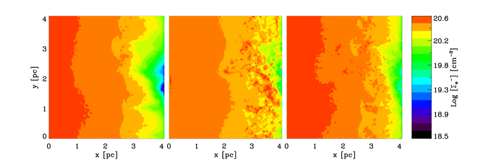
Figure 1: Surface density of electrons projected in the z-direction for the G09b turbulent ISM simulation at t = 0.5 Myr. Left: iVine; Middle: mocassin H-only; Right: mocassin nebular abundances.

3.1 Global Properties

Figure 1 shows the surface density of electrons projected in the z-direction for the G09b turbulent ISM simulation at t = 0.5 Myr. The figure shows that no significant differences are noticeable in the integrated ionisation structure, implying that the global ionisation structure is correctly determined by iVine. This is also confirmed by the comparison of the total ionised mass fractions: at t = 0.5 Myr, iVine obtains a total ionised mass of 13.9%, while mocassin “H-only” and “Metals” obtain 15.6% and 14.0%, respectively. The agreement at other time snapshots is equally good (e.g. at t = 250kyr iVine obtains 9.1% and mocassin “Metals” 9.5%).

It may at first appear curious that the agreement should be better between iVine and mocassin “Metals”, rather than mocassin “H-only”, given that only H-ionisation is considered in iVine. This is however simply explained by the fact that iVine adopts a “ionised gas temperature” ($T_{hot}$) of 10kK, which is close to a typical HII region temperature, with typical gas abundances. The removal of metals in the “H-only” simulations causes the temperature to rise to values close to 17kK, due to the fact that cooling becomes much less efficient without collisionally excited lines of oxygen, carbon etc. The hotter temperatures in the “H-only” models directly translate to slower recombinations, as the recombination coefficient is proportional to the inverse square root of the temperature. As a result of slower recombination the “H-only” grids have a slightly larger ionisation degree.

3.2 Ionisation and temperature structure

Figure 2: Density and temperature maps for the z = 25 slice of the G09 turbulent ISM simulation at t = 0.5 Myr. Top left: Gas density map; Top right: electron temperature, $T_{e}$ as calculated by iVine; Bottom left: electron temperature, $T_{e}$ as calculated by mocassin with H-only; Bottom right: electron temperature, $T_{e}$ as calculated by mocassin with nebular abundances.

Accurate gas temperatures are of prime importance as this is how feedback from ionising radiation impacts on the hydrodynamics of the system. In Figure 2 we compare the electron temperatures $T_{e}$ calculated by iVine and mocassin (“H-only” and “Metals”) in a z-slice of the t = 0.5 Myr grid. The top-right panel shows the number density [cm^-3] map for the selected slice. The large shadow regions behind the high density clumps are immediately evident from both figures. These shadows are largely reduced in the mocassin calculations as a result of diffuse field ionisation. The diffuse field is softer than the stellar field and therefore temperatures in the shadow regions are lower. The higher temperatures in the shadow regions of the mocassin “Metals” model are a consequence of the Helium Lyman radiation and the heavy elements free-bound contribution to the diffuse field. The rise in gas temperature shown in the mocassin results at larger distances from the star is not surprising and a simple consequence of radiation hardening and the recombining of some of the dominant cooling ions.

4 Towards more realistic algorithms

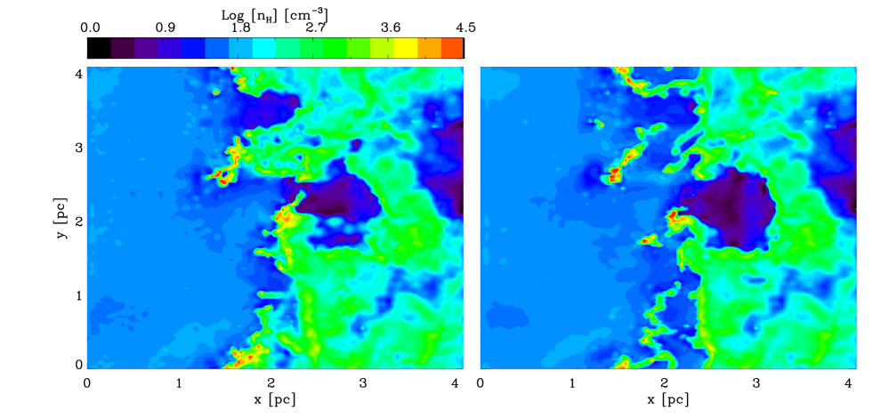
Figure 3: Density slice at 250 kyr for the OTS iVine (left) and the diffuse field iVine (right).

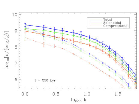
Figure 4: Turbulence spectrum obtained for the standard OTS iVine (solid lines), the control run with no ionising radiation (dotted line) and the diffuse field iVine (dashed lines).

As iVine solves the transfer along plane parallel rays, it has currently no means of bringing ionisation (and hence heating) to regions that lie behind high density clumps. This creates a large temperature (pressure) gradient between neighbouring direct and diffuse-field dominated regions, which may have important implications for the dynamics, particularly with respect to turbulence calculations. The same problem is faced by all codes that employ the OTS approximation and thus ignore the diffuse field contributions.

In order to investigate whether the error introduced by OTS approximation actually bears any consequence on the dynamical evolution of the system and on the turbulence spectrum, we propose here a simple zeroth order strategy to include the effects of the diffuse field in iVine and which can be readily extended to other codes. It consists of the following steps: (i) identify the diffuse field dominated regions (shadow); (ii) study the realistic temperature distribution in the shadow region using fully frequency resolved three-dimensional photoionisation calculations performed with mocassin and parameterise the gas temperature in the shadow regions as a function of (e.g.) gas density; (iii) implement the temperature parameterisation in iVine and update the gas temperatures in the shadow regions at every dynamical time step accordingly.

We note that this approach allows for environmental variables, such as the hardness of the stellar field and the metallicity of the gas to be accounted for in the SPH calculation, since their effect on the temperature distribution is folded in the parameterisation obtained with mocassin.

Figure 3 shows a slice of the density structure snapshots at 250k year for a standard ivine (left panel) compared to a first attempt at a diffuse field implementation in iVINE (right panel). These preliminary results indicate that the diffuse field affects the evolution of structures, promoting the detachment of clumps from the pillars, presumably by excavating them from behind.. Slightly higher densities are achieved in some of the clumps in the diffuse field simulation at this age, suggesting that the formation of stars may be thus accelerated. The turbulence spectrum obtained in simulations with or without diffuse fields are rather similar, as shown in Figure 4, where the specific kinetic energy is plotted as a function of wave number in the case of the control run with no ionisation at all (dotted lines), OTS iVine (solid lines) and diffuse field iVine (dashed lines). There is however tentative evidence for less efficient driving at the smaller scales, due to the fact that the large temperature gradients created by the OTS at the shadow regions are removed when the diffuse field is considered.

We stress that the results presented here are to be considered only a first exploratory step to establish whether diffuse field effects are likely to play a role in the dynamical evolution of a turbulent medium. More detailed comparisons will be presented in a forthcoming article (Ercolano & Gritschneder 2010, in prep)

5 Conclusions

We have presented a review of the current implementations of photoionisation algorithms in star formation hydrodynamical simulation, highlighting some of the most common approximation that are employed in order to simplify the radiative transfer and photoionisation problems.

We discuss the robustness of the temperature fields obtained by such methods in light of recent tests against detailed 3D photoionisation calculations for complex density distributions typical of star forming regions. We conclude that while the global ionised mass fractions obtained by the simplified methods are roughly in agreement, the temperature fields are poorly represented. In particular, the assumption of the OTS approximation may lead to unrealistic shadow regions and extreme temperature gradients that affect the dynamical evolution of the system and, to a lesser extent, its turbulence spectrum.

We propose a simple strategy to provide a more realistic description of the temperature distribution based on parameterisations obtained with a dedicated photoionisation code, mocassin, which includes frequency resolved 3D radiative transfer and all the microphysical process needed for an accurate calculation of the temperature distribution of ionised regions. This computationally inexpensive method allows to include the thermal effects of diffuse field, as well as accounting for environmental variables, such as gas metallicity and stellar spectra hardness.

References

- [Bertoldi(1989)] Bertoldi, F. 1989, ApJ, 346, 735
- [Bisbas et al.(2009)] Bisbas, T. G., Wünsch, R., Whitworth, A. P., & Hubber, D. A. 2009, A&A, 497, 649
- [Dale et al.(2005)] Dale, J. E., Bonnell, I. A., Clarke, C. J., & Bate, M. R. 2005, MNRAS, 358, 291
- [Dale et al.(2007)] Dale, J. E., Ercolano, B., & Clarke, C. J. 2007, MNRAS, 382, 1759
- [Elmegreen et al.(1995)] Elmegreen, B. G., Kimura, T., & Tosa, M. 1995, ApJ, 451, 675
- [Ercolano et al.(2003)] Ercolano, B., Barlow, M. J., Storey, P. J., & Liu, X.-W. 2003, MNRAS, 340, 1136
- [Ercolano et al.(2005)] Ercolano, B., Barlow, M. J., & Storey, P. J. 2005, MNRAS, 362, 1038
- [Ercolano & Storey(2006)] Ercolano, B., & Storey, P. J. 2006, MNRAS, 372, 1875
- [Ercolano et al.(2008a)] Ercolano, B., Young, P. R., Drake, J. J., & Raymond, J. C. 2008, ApJS, 175, 5345, 165
- [Garcia-Segura & Franco(1996)] Garcia-Segura, G., & Franco, J. 1996, ApJ, 469, 171
- [Goodwin & Bastian(2006)] Goodwin, S. P., & Bastian, N. 2006, MNRAS, 373, 752
- [Gritschneder et al.(2009)] Gritschneder, M., Naab, T., Walch, S., Burkert, A., & Heitsch, F. 2009, ApJL, 694, L26
- [Gritschneder et al.(2009)] Gritschneder, M., Naab, T., Burkert, A., Walch, S., Heitsch, F., & Wetzstein, M. 2009, MNRAS, 393, 21
- [Kessel-Deynet & Burkert(2000)] Kessel-Deynet, O., & Burkert, A. 2000, MNRAS, 315, 713
- [Klessen et al.(2009)] Klessen, R. S., Krumholz, M. R., & Heitsch, F. 2009, Advanced Science Letters (ASL), Special Issue on Computational Astrophysics, edited by Lucio Mayer, arXiv:0906.4452
- [Landi et al.(2006)] Landi, E., Del Zanna, G., Young, P. R., Dere, K. P., Mason, H. E., & Landini, M. 2006, ApJS, 162, 261
- [Mac Low(2007)] Mac Low, M.-M. 2007, proceedings of ”Massive Star Formation: Observations Confront Thoery”, ASP conference series, eds. H. Beuther et al., arXiv:0711.4047
- [Mellema et al.(2006)] Mellema, G., Arthur, S. J., Henney, W. J., Iliev, I. T., & Shapiro, P. R. 2006, ApJ, 647, 397
- [Miao et al.(2006)] Miao, J., White, G. J., Nelson, R., Thompson, M., & Morgan, L. 2006, MNRAS, 369, 143
- [Osterbrock & Ferland(2006)] Osterbrock, D. E., & Ferland, G. J. 2006, Astrophysics of gaseous nebulae and active galactic nuclei, 2nd. ed. by D.E. Osterbrock and G.J. Ferland. Sausalito, CA: University Science Books, 2006,
- [Peters et al.(2010)] Peters, T., Mac Low, M.-M., Banerjee, R., Klessen, R. S., & Dullemond, C. P. 2010, ApJ, 719, 831
- [Verner et al.(1996)] Verner, D. A., Ferland, G. J., Korista, K. T., & Yakovlev, D. G. 1996, ApJ, 465, 487
- [Yorke et al.(1989)] Yorke, H. W., Tenorio-Tagle, G., Bodenheimer, P., & Rozyczka, M. 1989, A&A, 216, 207