Relaxation Time and Dissipation Interaction in Hot Planet Atmospheric Flow Simulations

Abstract

We elucidate the interplay between Newtonian thermal relaxation and numerical dissipation, of several different origins, in flow simulations of hot extrasolar planet atmospheres. Currently, a large range of Newtonian relaxation, or “cooling”, times ($\sim$10 days to $\sim$1 hour) is used among different models and within a single model over the model domain. In this study we demonstrate that a short relaxation time (much less than the planetary rotation time) leads to a large amount of unphysical, grid-scale oscillations that contaminate the flow field. These oscillations force the use of an excessive amount of artificial viscosity to quench them and prevent the simulation from “blowing up”. Even if the blow-up is prevented, such simulations can be highly inaccurate because they are either severely over-dissipated or under-dissipated, and are best discarded in these cases. Other numerical stability and timestep size enhancers (e.g., Robert-Asselin filter or semi-implicit time-marching schemes) also produce similar, but less excessive, damping. We present diagnostics procedures to choose the “optimal” simulation and discuss implications of our findings for modeling hot extrasolar planet atmospheres.

1. Introduction

There are many studies using a “general circulation model” (GCM) to investigate the flow and temperature structure of close-in extrasolar planet atmospheres (e.g., Showman & Guillot, 2002; Cho et al., 2003; Cooper & Showman, 2005; Langton & Laughlin, 2007; Cho et al., 2008; Dobbs-Dixon & Lin, 2008; Showman et al., 2008; Menou & Rauscher, 2009; Thrastarson & Cho, 2010; Rauscher & Menou, 2010). GCMs are advanced numerical models that solve a set of coupled, nonlinear partial differential equations for the large-scale motions of a shallow fluid on a rotating sphere. In these sophisticated models, numerous parameters are needed to specify the representation of heating and cooling in the atmosphere and to stabilize the numerical integration.

Thus far, not much emphasis has been given to the numerical aspects of simulations in the extrasolar planet literature, in particular their influence on the accuracy of the model results. In an earlier paper, Thrastarson & Cho (2010) has investigated the sensitivity of initial condition on the extrasolar planet atmosphere flows. In this work, the focus is on another significant aspect—the subtle, and not so subtle, interplay between numerical and physical parameters. It should be noted that, while the discussion is basically numerical, this work is relevant to both theoretical studies and observations of extrasolar planets.

GCMs usually solve the hydrostatic primitive equations (see, e.g., Salby, 1996), which filter sound waves so that only two important classes of waves remain—Rossby, or planetary, waves (which evolve on slow time scales) and gravity waves (which generally evolve on time scales much shorter than the Rossby waves). The spatial scales of the two classes of motions are generally large and small, respectively. Nonlinear advection, which has often been used to define a time scale in extrasolar planet work so far, has roughly the same time scale as the Rossby waves. Generally, the amplitude of gravity waves, when averaged over the globe, is very small compared to that of Rossby waves, and most of the kinetic energy is contained in the large-scale, slow motions.

A long-standing challenge in GCM theory is finding ways to deal with fast waves accurately and efficiently. The fast motions not only force small timesteps to be taken (increasing the “wall time” of the simulations), they also degrade the fidelity with which the equations are solved. Moreover, the very inaccuracy often causes the calculation to “blow up” (become unstable), preventing any solution at all. With certain types of numerical algorithms, such as implicit or semi-implicit time-integration schemes, the timestep size restriction can be alleviated. But, artificial viscosity and various filters are still required to stabilize the integration in general.

It is well known that, in conjunction with coarse resolution, dissipation and filters can produce results that are seductively misleading—even to the wary modelers. For example, in the classic Held-Suarez test for the dynamical core of GCMs for the Earth (Held & Suarez, 1994), increasing the resolution generally leads to enhanced equatorward shift of wave activity (Wan et al., 2006). The shift becomes more evident in the simulations with horizontal resolutions  $\sim$$>$  T85 resolution (i.e., 85 sectoral and 85 total modes) so that precise jet positions, for example, cannot be ascertained at lower resolutions. This is a relatively mild example, but it is telling: the more extreme forcing condition for extrasolar planets, it can be argued, will lead to larger or more sensitive variations, given that the models have been designed and tested for conditions appropriate for solar system planets. In this backdrop, even inter-comparing different GCMs for extrasolar planet work becomes non-trivial.

In this paper we present and discuss examples of interesting behavior when a GCM is stressed to its limits, with what may be considered a typical hot, spin-orbit synchronized extrasolar planet condition. The implications are broad in the sense that the lessons are not just limited to studies using GCMs, but also other types of global circulation models. The issues are present in all of them.

The basic plan of the paper is as follows. In Section 2 we describe the GCM model we use and its setup for the simulations described in this work. In Section 3.1 we focus on the interaction between artificial viscosity and the thermal relaxation time, which is an important parameter in the representation of thermal forcing commonly used in current studies. In Section 3.2 we examine sensitivity of the simulations to the Robert-Asselin filter, which is used to stabilize the time-marching scheme. We conclude in Section 4, summarizing this work and discussing its implications for extrasolar planet circulation modeling.

2. Method

2.1. Governing Equations

In this work, we solve the same equations as in Thrastarson & Cho (2010). Here we briefly summarize the relevant aspects for the reader. The horizontal momentum equations are solved in the vorticity-divergence form:

$$\frac{{\partial}\zeta}{{\partial}t}\ = \ {\bf k}\cdot\mbox{\boldmath{$\nabla$}}\times{\bf n}+{\cal D}_{\zeta}$$ (1)

$$\frac{{\partial}\delta}{{\partial}t}\ = \ \mbox{\boldmath{$\nabla$}}\cdot{\bf n}+\mbox{\boldmath{$\nabla$}}^{2}(E+\Phi)+{\cal D}_{\delta},$$ (2)

where $\mbox{\boldmath{$\zeta$}}=\zeta\,{\bf k}=\mbox{\boldmath{$\nabla$}}\times{\bf v}$ is the vorticity, $\delta=\mbox{\boldmath{$\nabla$}}\cdot{\bf v}$ is the divergence, ${\bf v}$ is the horizontal velocity, ${\bf k}$ is the vertical unit vector, $E=({\bf v}\cdot{\bf v})/2$, $\Phi$ is the geopotential, and

$${\bf n}\ =\ -(\zeta+f)\,{\bf k}\times{\bf v}\,-\,\dot{\eta}\frac{{\partial}{\bf v}}{{\partial}\eta}\,-\,\frac{RT}{p}\mbox{\boldmath{$\nabla$}}p,$$

where $f$ is the Coriolis parameter, $p$ is pressure, $T$ is temperature and $R$ is the specific gas constant. The vertical coordinate is a generalized pressure coordinate, $\eta=\eta(p,p_{s})$, with $p_{s}$ the bottom surface pressure, and $\dot{\eta}\equiv{\rm D}\eta/{\rm D}t$ with

$$\frac{{\rm D}}{{\rm Dt}}\ \equiv\ \frac{{\partial}}{{\partial}t}\,+\,\mathbf{v}\!\cdot\!\mbox{\boldmath{$\nabla$}}\,+\,\dot{\eta}\frac{{\partial}}{{\partial}\eta}$$

the material derivative. Hydrostatic equilibrium is assumed:

$$\frac{{\partial}\Phi}{{\partial}\eta}\ =\ -\frac{RT}{p}\frac{{\partial}p}{{\partial}\eta},$$ (3)

and the ideal gas law, $p=\rho RT$, where $\rho$ is density, is taken as the equation of state. The mass continuity equation is integrated from the bottom ($\eta$ = 1) to the top surface, $\eta_{\rm t}$, using the boundary conditions $\dot{\eta}$ = 0 at both the top and the bottom, which yields an evolution equation for $p_{s}$:

$$\frac{{\partial}p_{s}}{{\partial}t}\ =\ \int_{1}^{\eta_{\rm t}}\mbox{\boldmath{$\nabla$}}\!\cdot\!\left(\frac{{\partial}p}{{\partial}\eta}{\bf v}\right)\,d\eta$$ (4)

Integration of the continuity equation from $\eta_{\rm t}$ to $\eta$ yields a diagnostic equation for $\dot{\eta}$:

$$\dot{\eta}\frac{{\partial}p}{{\partial}\eta}\ =\ -\frac{{\partial}p}{{\partial}t}\,-\,\int_{\eta_{\rm t}}^{\eta}\mbox{\boldmath{$\nabla$}}\!\cdot\!\left(\frac{{\partial}p}{{\partial}\eta}{\bf v}\right)\,d\eta.$$ (5)

The diagnostic equation for $\omega\equiv{\rm D}p/{\rm D}t$ is then:

$$\omega\ =\ {\bf v}\cdot\mbox{\boldmath{$\nabla$}}p\,-\,\int_{\eta_{\rm t}}^{\eta}\mbox{\boldmath{$\nabla$}}\!\cdot\!\left(\frac{{\partial}p}{{\partial}\eta}{\bf v}\right)\,d\eta.$$ (6)

Finally, the energy equation is

$$\frac{{\rm D}T}{{\rm D}t}\,-\,\frac{\omega}{\rho\,c_{p}}\ =\ \frac{\dot{q}_{\rm{\tiny net}}}{c_{p}}\,+\,{\cal D}_{T},$$ (7)

where $c_{p}$ is the specific heat at constant pressure. In the final formulation of the equations, terms involving ${\bf v}$ are represented in terms of the transformed velocity ${\bf v}cos\phi$, where $\phi$ is latitude, in order to avoid discontinuities at the poles. Also, the equations are formulated using ln($p_{s}$) instead of $p_{s}$ to avoid aliasing problems. The ${\cal D}$ terms in the vorticity, divergence and energy equations represent horizontal diffusion, discussed in the next subsection.

2.2. Numerical Algorithm

To solve the equations described in the preceding subsection, we use the Community Atmosphere Model (CAM 3.0), described in Collins et al. (2004) and Thrastarson & Cho (2010). CAM is a well-tested, highly-accurate hydrodynamics model employing the pseudospectral algorithm (Orszag, 1970; Eliasen et al., 1970).

For problems not involving sharp discontinuities (e.g., shocks or, in atmospheric dynamics problems, fronts) and irregular geometry, the pseudospectral method is superior to the standard grid and particle methods (e.g., Canuto et al., 1988). To equal the accuracy of the pseudospectral method for a problem solved with the computational domain decomposed into $N$ grid points, one would need a $N^{\rm th}$-order finite difference or finite element method with an error of $O(N\Delta x)$, where $\Delta x$ is the grid spacing and $O(\cdot)$ is the asymptotic order (e.g., Nayfeh, 1973). This is because as $N$ increases, the pseudospectral method benefits in two ways. First, $\Delta x$ becomes smaller, which would cause the error to rapidly decrease even if the order of the method were fixed. However, unlike finite difference and finite element methods, the order is not fixed: when $N$ is doubled to $2N$, the error becomes $O[(\Delta x)^{2N}]$ in terms of the new, smaller $\Delta x$. Since $\Delta x$ is $O(1/N)$, the error for the pseudospectral method is $O[(1/N)^{N}]$.

Significantly, the error decreases faster than any finite power of $N$ since the power in the error formula is always increasing as well, giving an “infinite order” or “exponential” convergence. This advantage is particularly important when many decimal places of accuracy or high resolution is needed. Note that in the vertical direction CAM uses a finite differencing scheme, as in most GCMs.

For the spherical geometry, the horizontal representation of an arbitrary scalar quantity $\xi$ consists of a truncated series of spherical harmonics,

$$\xi(\lambda,\mu)\ =\ \sum^{M}_{N(m)}\sum^{N(m)}_{n=|m|}\xi^{m}_{n}P^{m}_{n}(\mu)\,e^{im\lambda},$$

where $M$ is the highest Fourier (sectoral) wavenumber included in the east-west representation; $N(m)$, which can be a function of the Fourier wavenumber $m$, is the highest degree of the associated Legendre functions $P^{m}_{n}$; $\lambda$ is the longitude; and, $\mu\equiv\sin\phi$. The spherical harmonic functions,

$$Y^{m}_{n}(\lambda,\mu)\ =\ P^{m}_{n}(\mu)\,e^{im\lambda},$$ (8)

used in the spectral expansion are the eigenfunctions of the Laplacian operator in spherical coordinates:

$$\mbox{\boldmath{$\nabla$}}^{2}\,Y^{m}_{n}\ =\ -\left[\frac{n(n+1)}{R_{p}^{2}}\right]\,Y^{m}_{n},$$ (9)

where

$$\mbox{\boldmath{$\nabla$}}^{2}\ =\ \frac{1}{R_{p}^{2}}\left\{\frac{{\partial}}{{\partial}\mu}\left[\left(1-\mu^{2}\right)\frac{{\partial}}{{\partial}\mu}\right]\,+\,\frac{1}{1-\mu^{2}}\frac{{\partial}^{2}}{{\partial}\lambda^{2}}\right\}$$

and $R_{p}$ is the planetary radius. The set, $\{Y^{m}_{n}\}$, constitutes a complete and orthogonal expansion basis (Byron & Fuller, 1992).

In the Navier-Stokes equations, the diffusion terms appear as the Laplacian of the dynamical variables (Batchelor, 1967). In our case, the diffusion is generalized to the following “hyperdissipation” form (e.g., Cho & Polvani, 1996):

$${\cal D}_{\chi}\ =\ \nu_{2\mathfrak{p}}\left[(-1)^{\mathfrak{p}+1}\mbox{\boldmath{$\nabla$}}^{2\mathfrak{p}}+{\cal C}\right]\,\chi,$$ (10)

where $\chi=\{\zeta,\delta,T\}$ and ${\cal C}=(2/R_{p}^{2})^{\mathfrak{p}}$ is a correction term added to the vorticity and divergence equations to prevent damping of uniform rotations for angular momentum conservation. In the above form, the $\mathfrak{p}=2$ case is sometimes referred to as superdissipation. Hyperdiffusion is added in each layer to prevent accumulation of power on the small, poorly-resolved scales and to stabilize the integration.

Cho & Polvani (1996) describes the effects of various hyperviscosities (i.e., different values of $\mathfrak{p}$). As discussed in that work, a rational procedure for estimating roughly the value of $\nu_{2\mathfrak{p}}$ can be obtained in the following way. To damp oscillations at the smallest resolved scale (set by the truncation wave number, $n_{t}$), by an $e$-folding factor in time $\tau_{d}$, one requires that

$$\nu_{2\mathfrak{p}}\ =\ O\left\{\frac{1}{\tau_{d}}\left[\frac{R_{p}^{2}}{n_{t}(n_{t}+1)}\right]^{\mathfrak{p}}\right\}.$$ (11)

Thereafter, the optimal value of $\nu_{2\mathfrak{p}}$ is obtained by computing the kinetic energy spectrum (see Section 3). Note that the precise value is problem specific, and the procedure just described should be performed for each problem—as has been done in this work.

In numerical solutions of time-dependent equations, there are two main ways of marching in time. Explicit methods give the solution at the next time level in terms of an explicit expression which can be evaluated by using the solution at the previous timestep. Implicit methods, on the other hand, require solving a boundary value problem at each timestep. Explicit time differencing is a more straightforward numerical approximation to the equations. In our model, the time-marching is effected using a semi-implicit scheme, a mixture of the two methods commonly used in GCMs. In this scheme, the equations are split into nonlinear and linear terms, symbolically written:

$$\frac{{\partial}\Psi}{{\partial}t}\ =\ \mathcal{N}(\Psi)\,+\,\mathcal{L}(\Psi),$$ (12)

where $\mathcal{N}(\Psi)$ and $\mathcal{L}(\Psi)$ denote the nonlinear and linear terms, respectively, and $\Psi$ is the state of a variable in $\chi=\{\zeta,\delta,T\}$.

For the nonlinear terms, an explicit leapfrog scheme is used. This is a second-order, three-time-level scheme. Because a second-order method is applied to solve a differential equation which is first-order in time, an unphysical computational mode is admitted, in addition to the physical one. In simulations containing nonlinear waves, the computational mode can amplify over time, generating a time splitting instability (Durran, 1999). Robert (1966) and Asselin (1972) designed a filter to suppress the computational mode—hence the time splitting instability. This filter is applied in the GCM used in the present work. It is applied at each timestep so that

$$\bar{\Psi}^{\mathfrak{n}}\ =\ \Psi^{\mathfrak{n}}\,+\,\epsilon\left(\bar{\Psi}^{\mathfrak{n}-1}-2\Psi^{\mathfrak{n}}+\Psi^{\mathfrak{n}+1}\right),$$ (13)

where $\Psi^{\mathfrak{n}}=\Psi(\mathfrak{n}\Delta t)$, an overbar refers to the filtered state, and $\epsilon$ specifies the strength of the filter. The filter results in strong damping of the amplitude of the spurious computational mode. However, it also introduces a second-order error in the amplitude of the physical mode with high values of $\epsilon$, as we discuss further in Section 3.2.

Some parts of the equations can be solved implicitly with advantage. In particular, the linear parts that produce fast gravity waves are treated implicitly in many GCMs, including the one used in this work. This treatment allows a larger timestep to be used, as mentioned in Section 1. However, it is also at the cost of degraded accuracy (e.g., Durran, 1999).

As can be seen, time-integration of the primitive equations is not a straightforward matter, even with a relatively simple method like the leapfrog scheme. The theoretical analysis of the scheme is equally complex. The stability of the combined, semi-implicit leapfrog scheme has been examined by Simmons et al. (1978), particularly with respect to the basic state temperature profile. They find the isothermal basic state distribution to be more stable than a spatially-varying distribution, with the stability generally increasing with higher basic temperature. In the present work an isothermal basic state of 1400 K is used.

2.3. Calculation Setup

In addition to tuneable parameters associated with the numerical scheme, such as the ones mentioned in the preceding subsection, the representations of physical processes also require specification of parameters. Many of these are as yet poorly constrained by observations or unobtainable from first principles (see, e.g., discussions in Cho et al. (2008), Showman et al. (2008), and Cho (2008)). One example is thermal forcing (i.e., heating and cooling) due to the irradiation from the host star and radiative processes in the planetary atmosphere, which is represented in an idealized way currently in all extrasolar planet atmosphere simulations. Many crudely represent the forcing by Newtonian relaxation, as in this work (e.g., Cooper & Showman, 2005; Langton & Laughlin, 2007; Showman et al., 2008; Menou & Rauscher, 2009; Rauscher & Menou, 2010; Thrastarson & Cho, 2010).

In this representation, the net heating term in equation (7) is represented by

$$\frac{\dot{q}_{\rm{\tiny net}}}{c_{p}}\ =\ -\frac{1}{\tau_{\rm th}}\left(T-T_{e}\right),$$ (14)

where $T_{e}=T_{e}(\lambda,\phi,\eta,t)$ is the “equilibrium” temperature distribution and $\tau_{\rm th}$ is the thermal relaxation (drag or “cooling”) time. The appropriate values to use for this relaxation time (as well as the equilibrium temperature distribution) are poorly known and a large range of values has been used in the extrasolar planet literature. In several studies, very short relaxation times—even less than an hour—and large $T_{e}$ gradients have been used (e.g., Showman et al., 2008; Rauscher & Menou, 2010; Thrastarson & Cho, 2010). This represents a rather “violent” forcing on the flow, depending on the initial condition.

In this work, both $\tau_{\rm th}$ and $T_{e}$ are prescribed and barotropic (i.e., ${\partial}/{\partial}\eta=0$) and steady (i.e., ${\partial}/{\partial}t=0$). As in Thrastarson & Cho (2010),

$$T_{e}\ =\ T_{m}+\Delta T_{e}\cos\phi\cos\lambda\,,$$ (15)

with $T_{m}=(T_{D}+T_{N})/2$ and $\Delta T_{e}=(T_{D}-T_{N})/2$, where $T_{D}$ and $T_{N}$ are the maximum and minimum temperatures at the day and night sides, respectively. All the simulations described in this paper have $T_{D}=1900$ K, $T_{N}=900$ K. Other physical parameters chosen are based on the close-in extrasolar planet, HD209458b (see Table 1).

Table 1Physical Parameters

Planetary rotation rate	$\Omega$	2.1$\times$10-5	s-1
Planetary radius	$R_{p}$	108	m
Gravity	$g$	10	m s-2
Specific heat at constant pressure	$c_{p}$	1.23$\times$104	J kg-1 K-1
Specific gas constant	$R$	3.5$\times$103	J kg-1 K-1
Mean equilibrium temperature	$T_{m}$	1400	K
Equilibrium substellar temperature	$T_{D}$	1900	K
Equilibrium antistellar temperature	$T_{N}$	900	K
Initial temperature	$T_{0}$	1400	K

The spectral resolutions in the horizontal direction for the runs described in the paper are T85 and T21. The number refers to the maximum total wavenumber, $n_{t}=\max\{N(m)\}$, at which expansion (8) is truncated (e.g., T85 $\ \Rightarrow\ n_{t}=85$); “T” means the truncation is such that $M=N$ in equation (8), a “triangular truncation” in wavenumber space. A T85 spectral resolution corresponds roughly to 800$\times$400 grid points in physical space of grid-based methods (roughly 200$\times$100 for T21 resolution). The vertical direction is resolved by 26 coupled layers, with the top level of the model located at 3 mbar. The pressure at the bottom $\eta$ boundary is initially 1 bar, but the value of the pressure changes in time. The entire domain is initialized with an isothermal temperature distribution, $T_{0}=T_{m}=1400$ K. The flow field is initialized with a small, random perturbation; specifically, values of the ${\bf v}$ components are drawn from a Gaussian random distribution centered on zero with a standard deviation of 0.05 m s^-1. The sensitivity to initial flow is described in detail in Thrastarson & Cho (2010).

3. Results

3.1. Spatial Dissipation

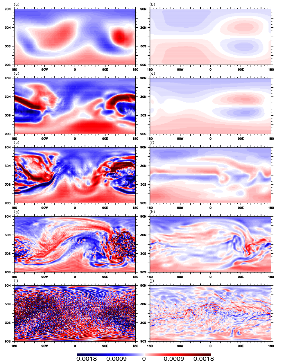
Figure 1.— Vorticity field at $t=80\,\tau_{p}$ (planet rotations), near the $p\approx 85\!$ mb level, for two sets of five simulations (left column and right column) that are set up identically, except for the viscosity coefficient and the thermal relaxation time. The global kinetic energy time series for all the runs have reached stationary (“equilibrated”) states and do not qualitatively change for $\sim\!300\,\tau_{p}$. The superdiffusion coefficient is $\nu_{4}=\{10^{24},10^{23},10^{22},10^{21},10^{20}\}$ m⁴ s^-1, decreasing from top to bottom in each column. The panels in the left column have a relaxation time of $\tau_{\rm th}=0.1\,\tau_{p}$ while the panels on the right have $\tau_{\rm th}=3\,\tau_{p}$. Red (blue) color represents positive (negative) values of vorticity, with units $s^{-1}$.

Table 2 lists all the runs discussed in this subsection. Simulations are performed with the setup described above, but with varying strength of artificial viscosity ($\nu$ and $\mathfrak{p}$) and the forcing timescale ($\tau_{\rm th}$). Figure 1 presents the relative vorticity field near the $p\approx 85\!$ mb level; this is approximately a quarter of the way down from the top of the computational domain. The field at $t=80\,\tau_{p}$ is shown in cylindrical equidistant projection, centered at the equator, for ten simulations in which the setup is identical except for the values of $\tau_{\rm th}$ and $\nu$ ($\mathfrak{p}=2$, superdissipation); here, $\tau_{p}=2\pi/\Omega$ is the planetary rotation period. Positive vorticity (red color) signifies local rotation in the same direction as the planetary rotation (counter-clockwise in the northern hemisphere), and opposite for the negative vorticity. The panels on the left column all have the same short value of $\tau_{\rm th}=0.1\,\tau_{p}$, while the panels on the right column all have $\tau_{\rm th}=3\,\tau_{p}$ for five different values of $\nu$. In all the runs shown, the global kinetic energy time series have reached stationary (“equilibrated”) state and do not change qualitatively for approximately 300$\,\tau_{p}$.

For a given value of $\tau_{\rm th}$, simulations with different $\nu$’s generally share some common features over a range of $\nu$’s. But, there are clear differences in the character of the flow and temperature fields. The differences, which are both qualitative and quantitative, arise from the strength of dissipation. Moreover, $\nu$ can affect the temporal behavior as well. For example, temporal variability can be muted with larger $\nu$. Not surprisingly, in the strongest dissipation cases [panels (a) and (b)] variability in time is essentially completely quenched and the flow structures are quite smooth in appearance. These are examples of runs which are severely over-dissipated.

At the other extreme, runs can also be severely under-dissipated. This is shown in panels (i) and (j) in Figure 1. Note that the common $\nu$ value in these runs is four orders of magnitude smaller than that for the runs of panels (a) and (b). A quick visual check of panels (i) and (j) immediately shows the physical fields dominated by small-scale oscillations: this is numerical noise. Here, by “small” we mean scales near the grid-scale, $l=O(\Delta x)$. Typically, runs like these blow up—or at least they should (see Section 3.2). Simulations often blow up long before the small-scales contain any significant amount of energy compared to the large-scales. As we discuss more later, this is because the calculation correctly becomes unstable. But, sometimes misbehaving simulations can be surprisingly resilient and not crash. This is usually a signal that bad numerics is at play.

Table 2List of Runs Discussed

Run	$\nu_{2\mathfrak{p}}$ [m4 s-1]	$\mathfrak{p}$	$\tau_{\rm th}/\tau_{p}$
N1a	1$\times$1024	2	.1
N1b	1$\times$1024	2	3
N2a	1$\times$1023	2	.1
N2b	1$\times$1023	2	3
N3a	1$\times$1022	2	.1
N3b	1$\times$1022	2	3
N4a	1$\times$1021	2	.1
N4b	1$\times$1021	2	3
N5a	1$\times$1020	2	.1
N5b	1$\times$1020	2	3
N6a	†6$\times$1012	1	.1

Note. — $\nu$ is the hyperviscosity coefficient and $\mathfrak{p}$ the order index of the hyperviscosity. $\tau_{\rm th}$ is the thermal relaxation timescale and $\tau_{p}$ is one planet rotation. All the simulations are run at T85 resolution with a timestep $\Delta t$ of 60 s and a Robert-Asselin filter coefficient $\epsilon$ of 0.06.

^†The units for this $\nu$ are [m² s^-1].

As expected, increasing $\nu$ leads to decreasing small-scale oscillations and to increasingly smoother fields. However, significantly, we note that for a given value of $\nu$ for the two $\tau_{\rm th}$’s (cf., panels of the same row in Figure 1) shorter $\tau_{\rm th}$ in a run admits much more pronounced grid-scale oscillations. For example, with $\nu_{4}=10^{22}$ m⁴ s^-1 [panels (e) and (f)], the viscosity is clearly insufficient to suppress small-scale oscillations in the case of $\tau_{\rm th}=0.1\,\tau_{p}$, while no small-scale oscillations are present in the calculation with longer $\tau_{\rm th}$. More importantly, a $\nu$ value which appears to be acceptable for the shorter relaxation time [e.g., panel (a)] is clearly over-dissipative for the run with the longer $\tau_{\rm th}$ [e.g., panel (b)]: here, the calculation in (b) should be compared with that in (f), which is clearly a much less dissipated run than that in (b). Hence, running a simulation at a single $\tau_{\rm th}$—even if $\nu$ were varied—would not produce trustworthy results since the parameter space is at least two-dimensional.

The implication of this is serious. In many current simulations of hot planet atmospheric flows, a range of $\tau_{\rm th}$’s is specified, spread over the model atmosphere domain, which always contains a region with a short $\tau_{\rm th}$. This forces those model atmosphere calculations to be excessively noisy and excessively dissipated, in different atmospheric regions of the computational domain. Once noise appears in the calculation somewhere in the domain, the entire domain becomes quickly contaminated. Note that an inherently smooth field—such as temperature compared to vorticity, for example—would not reveal the noise as well, since it is essentially two integrations (a smoothing operation) of the vorticity field. In other words, temperature possesses a steep (narrow) spectrum like the stream function, as opposed to a shallow (broad) spectrum like the vorticity. Similarly, other averaging (integrating) procedures, such as taking zonal (eastward) and/or temporal means, would obscure, possibly mislead, the analysis of the simulation if unaveraged “higher-order” fields like vorticity are not considered concomitantly.

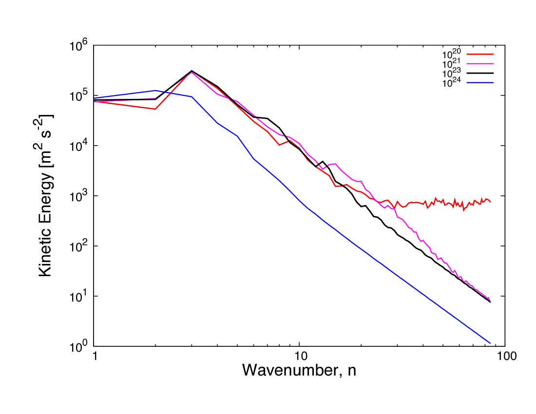
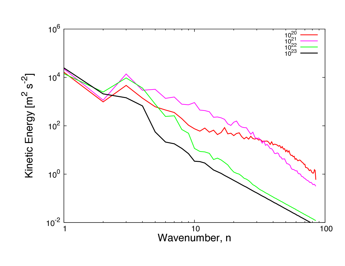
Figure 2.— Kinetic energy spectra for the fields shown in Figure 1 for simulations that are set up identically, except for the artificial viscosity and the thermal relaxation time. The runs shown in the left panel have a relaxation time of $\tau_{\rm th}=0.1\,\tau_{p}$ while the runs on the right panel have $\tau_{\rm th}=3\,\tau_{p}$. The different colored lines are for different values of $\nu$, as indicated in the legend. Note the different scales on the two panels—much more kinetic energy is contained in the flow when the relaxation time is short. The spectra reveal both under-dissipated (e.g. red line, left panel) and over-dissipated (e.g. blue line, left panel) flow fields. A $\nu$-value that seems to give a reasonable spectrum for the short $\tau_{\rm th}$ (e.g. black line, left panel) results in over-dissipation for the longer $\tau_{\rm th}$ (black line, right panel).

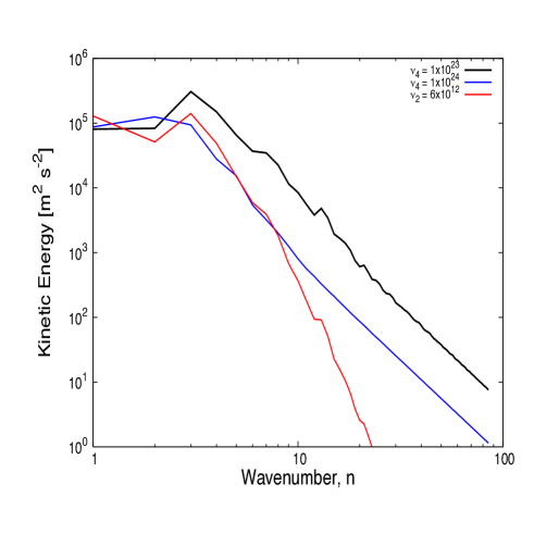
Figure 3.— Kinetic energy spectra for simulations that are set up identically, except for the artificial viscosity. The different lines refer to different values of $\nu$, as indicated in the legend. The blue and black lines are the same as in the left panel of Figure 2, for which the viscosity is of biharmonic form ($\mbox{\boldmath{$\nabla$}}^{4}$ with $\mathfrak{p}=2$). But, the red line is for a simulation where the order of the viscosity is lower ($\mathfrak{p}=1$), the normal Newtonian viscosity.

We wish to emphasize here that, in contrast to what might be the customary view, numerical noise and blow-ups are useful. Simulations with severe forcing should be allowed to crash—or at least halted, when near grid-scale oscillations are visible in the flow field. Any phenomena observed thereafter would be seriously compromised in accuracy, and quite possibly entirely artifactual (Boyd, 2000). In numerical work, it is easy to get lured into believing a calculation by not heeding important telltale signs.

There is a rational way to diagnose the onset of the small-scale error sources—as well as the excessive dissipation—in a simulation. This is illustrated in Figure 2, which contains the kinetic energy spectra of the fields presented in Figure 1. To the best of our knowledge, this is the first time kinetic energy spectra are shown in extrasolar planet atmosphere flow simulations. They provide an important diagnostic, when used in conjunction with instantaneous fields (see, e.g., Cho & Polvani (1996) and Koshyk et al. (1999) for a discussion of kinetic energy spectra and horizontal diffusion), and can be used to choose an appropriate $\nu$ value.

The left set of spectra in Figure 2 corresponds to runs with the shorter $\tau_{\rm th}~{}=~{}0.1\,\tau_{p}$ in the left column of Figure 1, and the right set of spectra in Figure 2 corresponds to runs with the longer $\tau_{\rm th}~{}=~{}3\,\tau_{p}$ in the right column of Figure 1. Visual inspection of the vorticity fields along the left column of Figure 1 suggests the runs in panels (a) and (c) are not much affected by the small-scale oscillations [if at all in the run of panel (a)]. This can be quantified by confirming that the corresponding spectra in Figure 2 (left panel) are the blue and black lines (runs N1a and N3a, respectively). In fact, the blue line clearly reveals a case of over-damping, in which all scales are less energetic than the corresponding scales in the other runs.

In contrast, note the appearance of near-grid-scale waves in physical space, for the run in panel (i) in Figure 1, indicated by a tendency for the spectrum (red line in left panel of Figure 2) to peel off and curl up near—and considerably to the left (larger scale) of—the aliasing limit; this is

$$n_{a}\ =\ \frac{2\pi R_{p}}{3\Delta x},$$

which is $\approx 85$ in our case, since $\Delta x$ is chosen to be “alias-free” up to $n_{t}$ (Orszag, 1971). Clearly, our de-aliasing procedure, of inverse transforming onto a physical grid that is $3n_{t}+1$ around the longitude, is not successful in runs N5a and N4a, as well as in run N3a (spectrum not shown). This is because increasingly greater resolution is needed as the calculation proceeds, as discussed below. In turbulence simulations, this peeling off behavior is known as an “energy pile-up” or “spectral blocking” (because direct energy cascade to high wavenumbers in three-dimensional turbulence is blocked). It is not limited to spectral methods. It is universal to all methods which discretize space.

Spectral blocking can cause numerical instability in the time integration of any nonlinear equations. The instability arises due to the quadratically nonlinear term in the solved equations. For example, a typical quadratically nonlinear term (in one-dimensional Cartesian geometry for simplicity) gives:

$$\psi\frac{{\partial}\psi}{{\partial}x} \ =\ \left(\sum^{K}_{p=-K}a_{p}\,e^{ipx}\right)\!\cdot\!\left(\sum^{K}_{q=-K}i\,q\,a_{q}\,e^{iqx}\right)=\sum^{2K}_{k=-2K}b_{k}\,e^{ikx}.$$

Here, $\psi(x,t)$ is an arbitrary one-dimensional scalar function, which is Fourier expanded; $b_{k}$ are given by a sum over the products of the $a_{k}$; $K$ is the truncation wavenumber, corresponding to $n_{t}$ in equation (11). Note that the nonlinear interaction generates high wavenumbers, $k>K$, which will be aliased into wavenumbers on the range $k\in[-K,K]$. This induces an unphysical inverse cascade of energy from high wavenumbers to low wavenumbers.

It is important to realize that the above cascade injects artificial energy into all scales. The injection is simply more noticeable in the small scales since not much energy is contained there in the absence of blocking. Oscillations of size $l=O(\Delta x)$ are a precursor to breakdown of computational fidelity. These oscillations are insidious because they require higher and higher resolution in the calculation over time. Without the increasing resolution, they deteriorate the accuracy of the simulation on all scales as the calculation proceeds, as pointed out in Thrastarson & Cho (2010). Although some blocking is almost inevitable in a long time integration of a nonlinear system (unless the dissipation is unrealistically large), it can be monitored and controlled—albeit better in some methods than in others.

The left and right panels of Figure 2 reveal not only how the appropriate dissipation can be chosen, but also the crucial interplay between the small-scale noise and $\tau_{\rm th}$—hence, underscoring the importance of using both the spectra and the physical field in analyzing a calculation. Consider, for example, the “optimal” calculation (i.e., least affected by too much or too little dissipation) for the short $\tau_{\rm th}$ runs. The calculation with $\nu_{4}=10^{23}$ m⁴ s^-1 (black line in the left panel) is devoid of non-physical build up of energy at the smallest scales while still retaining the same amount of energy in the large scales as in the calculations with smaller $\nu$. On the other hand, the calculation with longer $\tau_{\rm th}$ but same $\nu$ (black line in the right panel) is clearly over-dissipated, containing less energy compared to the other calculations on essentially all the scales. Hence, if the $\nu$ value were “tuned” with the calculations with shorter $\tau_{\rm th}$ (only), then a calculation with a different $\tau_{\rm th}$ (say a longer one, as in this example) would be over-damped. In other words, a correct $\nu$ value cannot be obtained independent of $\tau_{\rm th}$. Actually, $\nu=\nu\,(\tau_{\rm th},\epsilon,\cdots)$, where “$\cdots$” includes $T_{e}$, $R_{p}$. semi-implicitness, etc.

The above behavior is generic. Simulations performed with a greater range of $\tau_{\rm th}$ (down to 0.01 $\tau_{p}$) and $\nu$ and $\mathfrak{p}$, exhibit the same basic behavior; and, it is present throughout the model domain; grid-scale oscillations can appear in the duration of a calculation anywhere in the domain. These oscillations can be controlled to some degree in mild cases, as outlined above. However, grid-scale oscillations are dominant near the top of the domain for all values of $\nu$ considered. In this situation, it is common in GCM studies to include a “sponge layer”, where dissipation is artificially enhanced in the topmost layers. While this can damp unphysical oscillations, it can also have spurious effects. The effects of “sponges” as well as other boundary conditions will be described elsewhere.

Figure 3 shows how the spectrum is affected when the form of the artificial viscosity is of lower order. The blue and black lines (runs N1a and N2a, respectively) are the same as in the left panel of figure Figure 2. They can be compared to the red line (run N6a), which shows the spectrum from a simulation that is identical to the other two runs in the figure, except for the value of $\nu$ and the order of the viscosity operator (here $\mathfrak{p}=1$). In this case, the energy in the small scales (high wavenumbers) is dissipated much more strongly. More importantly, essentially all wavenumbers are affected by the lower order viscosity; and, as discussed in Cho & Polvani (1996), the slope of the spectrum becomes steeper—even at wavenumbers well below the truncation scale.

3.2. Temporal Dissipation

If the solved equations support several types of waves, as with the primitive equations, the maximum stable timestep is limited by the Courant number,

$$\mu^{*}\equiv c_{\rm max}\left(\frac{\Delta t}{\Delta x}\right),$$

where $c_{\rm max}$ is the maximum horizontal wind speed associated with the fastest propagating wave. Some fast waves are of little physical significance, but they enslave $\Delta t$ to be small. Implicit schemes do permit a larger timestep size to be used than in explicit schemes, often making the former more computationally efficient. However, for nonlinear equations, implicit schemes have a high cost per timestep because a nonlinear boundary value problem must be solved at each timestep.

As noted, a semi-implicit algorithm is commonly used in GCMs. In general, the implicit and explicit parts in the algorithm may be of same or different order. Treating some terms explicitly while others implicitly may appear strange, but there are some major advantages. First, because the nonlinear terms are treated explicitly, it is only necessary to solve a linear boundary value problem at each timestep. Second, the hyperdissipation terms, which involve even number of derivatives, impose a much stiffer timestep requirement than the advective terms; for example, $\Delta t$ is $O(1/N^{4})$ and $O(1/N^{2})$, respectively, for the Newtonian viscosity ($\mathfrak{p}=1$). Hence, the semi-implicit algorithm stabilizes the most unwieldy terms. Third, in general circulation and other fluid dynamics problems, advection is crucial; therefore, it is important to use a high order time-marching scheme with a short timestep to accurately compute phenonmena or structures such as frontogenesis, advection of storm systems, and turbulent cascades. There is little advantage in treating the nonlinear terms implicitly because a timestep longer than the explicit advective stability limit would be too inaccurate.

Note that, although it is possible to treat the time coordinate spectrally, it is generally more efficient to apply spectral methods to the spatial coordinates only because time marching is usually much cheaper than computing the solution simultaneously over all space-time. In general, much less concern is given to the temporal accuracy than the spatial accuracy of GCMs—usually with good justification: spatial errors pose greater problems, especially for the short and medium range duration runs typically performed with the models. This obviously does not apply for long duration runs, particularly if quantitative predictions are sought (Thrastarson & Cho, 2010).

Table 3Summary of Runs for Time Filter Sensitivity

Run	$\ \ \ \epsilon$	$\tau_{\rm th}/\tau_{p}$	Notes
E1a	0.001	.1	blow-up ($t=1\,\tau_{p}$)
E1b	0.001	3	blow-up ($t=71\,\tau_{p}$)
E2a	0.002	.1	blow-up ($t=1\,\tau_{p}$)
E2b	0.002	3
E3a	0.006	.1	blow-up ($t=8\,\tau_{p}$)
E3b	0.006	3
E4a	0.01	.1
E4b	0.01	3
E5a	0.06	.1
E5b	0.06	3
E6a	0.1	.1
E6b	0.1	3

Note. — $\tau_{\rm th}/\tau_{p}$ is the thermal relaxation time in units of planetary rotations, and $\epsilon$ is the Robert-Asselin filter coefficient. All the runs are at T21 resolution and have $\nu_{4}$ = 10²² m⁴ s^-1. The timestep is $\Delta t$ = 240 s.

As already discussed, a computational mode arises in the leapfrog scheme, which is an example of a two-step scheme:

$$\Psi^{\mathfrak{n}+1}\ =\ \Psi^{\mathfrak{n}-1}\,+\,\mathcal{F}(\Psi^{\mathfrak{n}},\mathbf{x},t^{\mathfrak{n}};\epsilon),$$ (16)

where $\mathbf{x}\in\mathbb{R}^{2}$; recall that $\epsilon$ is the Robert-Asselin time filter coefficient. Computational modes arise in all multistep methods. Fortunately, in some multistep methods $\Delta t$ can be chosen to keep the amplitude of the modes from growing. However, the leapfrog scheme is unstable for diffusion, for all $\Delta t$. For this reason, the diffusion part of the equations is “time-lagged” by evaluating the diffusion terms at the time level $(\mathfrak{n}-1)$. This effectively time-marches the diffusion part by a first-order scheme.

The Robert-Asselin filtered leapfrog scheme has been analyzed by Durran (1991) for the simple oscillation equation,

$$\frac{{\rm d}\psi}{{\rm d}t}\ =\ i\omega\psi,$$ (17)

where $\omega$ is the frequency of oscillation. That analysis shows that, in the limit $\omega\Delta t\ll 1$, the relative phase-speed error of the physical mode is

$${\cal R}_{\rm phys}\ =\ 1+\left[\frac{1+2\epsilon}{6\,(1-\epsilon)}\right](\omega\Delta t)^{2}.$$ (18)

Therefore, the phase of the numerical solution leads the actual solution in time, and the error increases with larger $\epsilon$. No analysis exists to guide in choosing $\epsilon$. Hence, it is important to assess the sensitivity of the simulations to the filter. In this work, we have performed series of simulations in which $\epsilon$ has been varied while keeping everything else fixed, for different values of relaxation time $\tau_{\rm th}$. The simulation parameters are summarized in Table 3.

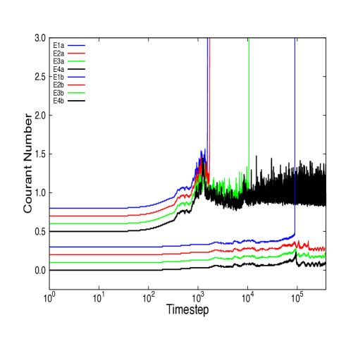
Figure 4.— Courant number as a function of time for two sets of runs with different values of $\tau_{\rm th}$ in each set. The four runs within each set have different $\epsilon$ values, setting the strength of the Robert-Asselin time filter. For clarity each time series in a set has been offset vertically by 0.1 in the plot; and, the two sets, as groups, have been offset vertically by 0.5. The lower set of runs have $\tau_{\rm th}$ = 3 $\tau_{p}$, while the upper set of runs have $\tau_{\rm th}$ = 0.1 $\tau_{p}$. For each set the run with $\epsilon$ = 0.001 is indicated with a blue line, $\epsilon$ = 0.002 a red line, $\epsilon$ = 0.006 a green line, and $\epsilon$ = 0.01 a black line.

Figure 4 shows the evolution of the Courant number $\mu^{*}$ for simulations with different $\epsilon$, for two sets of runs with different values of $\tau_{\rm th}$ in each set. Note that for clarity each time series in a set has been offset vertically by 0.1 in the plot; and, the two sets, as groups, have been offset vertically by 0.5. At the T21 resolution of the runs shown, for $\tau_{\rm th}=3\,\tau_{p}$ and $\nu=10^{22}$ m⁴ s^-1, it is found that a value of at least $\epsilon=0.002$ is needed to prevent the simulation from succumbing to time-splitting instability.

With shorter relaxation time ($\tau_{\rm th}=0.1\,\tau_{p}$), a larger value of $\epsilon$ is required for the simulation to proceed without blowing up; this is perhaps not surprising, in light of the preceding discussion. But, remarkably, even without explicit numerical viscosity turned on (i.e., $\nu$ set to 0), the simulation can proceed without crashing; and, this is so despite the fact that the physical field is completely swamped with noise! When $\tau_{\rm th}=3\,\tau_{p}$, runs do not crash as long as $\epsilon\geq 0.006$. However, with $\tau_{\rm th}=0.1\,\tau_{p}$, the minimum $\epsilon$ for not crashing is an order of magnitude greater. Evidently, an $\epsilon$ value used in earlier studies of Earth’s atmosphere should be adjusted when adapting an Earth GCM for extrasolar planet study. In general, a shorter $\tau_{\rm th}$ or lower viscosity requires stronger Robert-Asselin filtering to prevent blow-up.

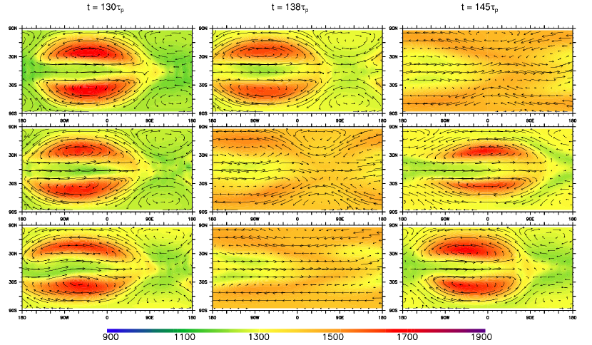
Figure 5.— Temperature (color coded in K) with streamlines overlaid, for three simulations differing only in the value of $\epsilon$, shown at three moments in time. From left to right, the snapshots are taken at $t=\{130,138,145\}\tau_{p}$. The top row is from a run with $\epsilon$ = 0.01, the middle row with $\epsilon$ = 0.06 and the bottom row $\epsilon$ = 0.10. All the fields are shown at the $p\approx 900\!$ mb level. The substellar point is at $0^{\circ}$ longitude and latitude.

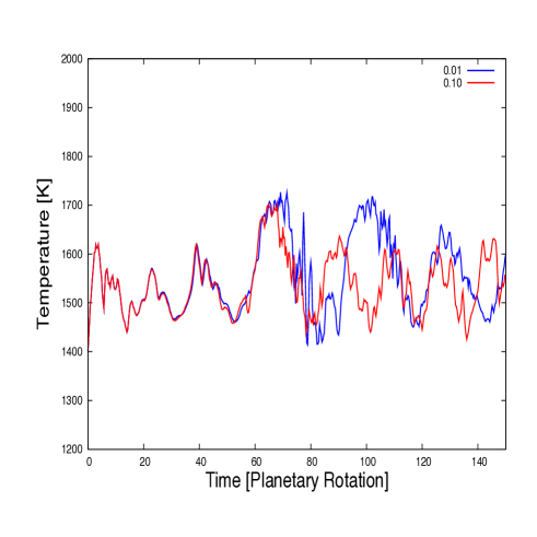
Figure 6.— Temperature at a fixed point, at 0^∘ longitude and 30^∘ latitude, as a function of time for the first 150 planet rotations in two simulations. The two curves show results of simulations that are identical apart only from the strength of the Robert-Asselin time filter. The red curve is from a run with $\epsilon$ = 0.10, and the blue curve from a run with $\epsilon$ = 0.01.

Note that the Courant-Friedrichs-Lewy (CFL) criterion for stability of the leapfrog scheme (Durran, 1999),

$$\mu^{*}\ \leq\ \frac{1}{\pi},$$

can sometimes be exceeded in the middle of a run, even though the simulation is stable at $t=0$ (cf., run E3a in Figure 4). This is because the advective time-stepping limit depends on the maximum speed $c_{\rm max}$, which can increase during the evolution of a flow. Careful monitoring of the physical fields shows a zone of intense shear between the two vortices generating small-scale oscillations that rapidly amplify until the simulation becomes nonsense. The culprit is not lack of spatial resolution or a blocked turbulent cascade, in this case, because the calculation can be extended indefinitely by halving the timestep.

Figure 5 illustrates the sensitivity of the evolution to $\epsilon$ for the range, $\epsilon\in[0.01,0.1]$. Although the resolution in these calculations is only T21, they illustrate the point. Snapshots of the flow field are shown at three successive times for three simulations, differing only in the value of $\epsilon$. Similar flow patterns emerge in all the simulations: they all exhibit a cyclic behavior with vortices translating around the planet, undergoing large variations in strength and size as they do so, with corresponding changes in the temperature field. However, at a given instant the flow and temperature fields look different between the three runs. At $t=130\,\tau_{p}$, in all the runs there is a warm cyclone pair centered west of the substellar point. And in all the runs, the cyclones move westward and the flow and temperature fields undergo substantial changes before eventually returning to a similar state, 15–20 planet rotations later. But at $t=145\,\tau_{p}$, the run with the largest $\epsilon$ has already returned to a state similar to that at $t=130\,\tau_{p}$, while the runs with smaller $\epsilon$ take longer to complete their cycles.

Figure 6 shows the behavior more clearly. The temperature at a point on the model planet atmosphere (0^∘ longitude, 30^∘ latitude) evolves in time for two simulations which have identical parameters, except for $\epsilon$. The two runs match nearly exactly until about 45$\,\tau_{p}$, when the two runs start to deviate. In the beginning only slightly. But, at about 70$\,\tau_{p}$ the temperature oscillations in the run with the larger $\epsilon$ lead in phase, compared to the run with smaller $\epsilon$. This behavior agrees qualitatively with Equation 18. Over long timescales the three simulations exhibit very similar behavior, even if amplitudes, phases, and periodicities of the flow and temperature fields are not exactly the same. As noted, simulations shown in Figures 5 and 6 are at T21 resolution, but with higher resolution deviations appear even earlier.

In Showman et al. (2009), the MITgcm (Adcroft et al., 2004) is used. In that study, the model employs the third-order Adams-Bashforth method, which has some attractive properties (Durran, 1991). However, the scheme does require an initialization phase in which $\Psi^{1}$ and $\Psi^{2}$ are computed from the initial condition $\Psi^{0}$ by some other procedure, such as the fourth-order Runge-Kutta or a first- or second-order scheme with several short timesteps. It should be emphasized that—as it is a major point of this paper—the main concern is usually adequate spatial resolution, especially in problems with inherent small-scale phenomena, not the time-integration. A second- or even first-order time-integration scheme can be perfectly adequate for many purposes.

4. Conclusion

A major aim of this paper has been to shed light on some crucial aspects for numerical modeling of atmospheric circulation on hot extrasolar planets. Here we have shown that, a spectral model offers advantages in accuracy and diagnostics, given that the higher-order field and wavenumbers are what’s actually evolved. However, all numerical models, including spectral models, have limitations in how well they can represent physical reality. Moreover, the models can easily be applied outside the realm of “safe parameters” and produce results that are nonsensical. The challenge is to properly test and identify the limits. When numerical artifacts appear, it is important to know how to deal with them and to know when a simulation should be discarded.

In this paper we have shown that, for hot extrasolar planets simulations with stationary forcing, there is a strong sensitivity to the strength of applied artificial viscosity. In addition, there is a relation between the thermal relaxation time $\tau_{\rm th}$ and the viscosity $\nu$: small $\tau_{\rm th}$’s lead to a large amount of unphysical, grid-scale oscillations in the simulation, which forces the use of excessive amounts of artificial viscosity to quench the oscillations. Hence, using a fixed strength of artificial viscosity in a simulation with a large range of $\tau_{\rm th}$ in the model domain (e.g., from about an hour to tens of days)—as done in many simulations in the literature—inevitably produces flow and temperature fields, which are either dominated by unphysical noise or over-damping. One may then wish to apply a spatially varying $\nu$, but clearly this is then motivated by a numerical basis rather than a physical one.

The proper values to use for the relaxation time (or variables needed for realistic radiative transfer) are not known. Based on the findings in this work, calculations with extremely short $\tau_{\rm th}$’s warrant further scrutiny. Current GCMs may not be standing up too well to this stressful test. If, however, the short $\tau_{\rm th}$ are really physically relevant, then another form of heating/cooling parameterization or setup is needed. This is not a criticism of the Newtonian relaxation scheme, which in fact has been (and continues to be) very useful for understanding basic mechanisms.

One solution could be to spatially vary the $\nu$, as already discussed; but, this would lead to further complexity. Even if direct radiative transfer is incorporated, one must ensure that the forcing is not too violent or strong (large amplitude and short timescale). Indeed, a comparison of our $\nu$ values, scaled appropriately for the Earth, shows that we have had to use $\nu$ values higher than that normally used in Earth studies (Collins et al., 2004). As discussed in (Cho, 2008), if the radiative processes appear as practically instantaneous from the perspective of the flow, then an adiabatic approach is more appropriate. Certainly from a numerical accuracy standpoint, as motivated by the present work, adiabatic and “gently forced” calculations are useful as baselines. Else, gradually ramping up heating and/or initializing simulations close to a balanced state is necessary (Thrastarson & Cho, 2010).

GCMs of extrasolar planet atmospheres have great value in helping to guide and interpret observations. It is then important to critically examine the effects of the numerous parameters that are specified. This is particularly crucial when applying the models to a “new regime”, where the physical conditions differ markedly from a traditional (e.g., Earth) one. In this paper we have shown examples of how a commonly-used forcing can steer GCMs to produce misleading results and how numerical expediencies, such as the Robert-Asselin filter, can produce slewing frequency as well as the well-known damping and phase-errors (Durran, 1991; Williams, 2009). In addition, we have discussed diagnostics procedures to better assess the quality of a simulation using the vorticity field and energy spectra. Reliance on spatial and temporal averages can effectively conceal telltale signs that a simulation is not trustworthy.

A simulation which is properly resolving the flow should approximately conserve energy for a long time. This should be so even if this property is not explicitly built into the discretization algorithm as in the scheme of Arakawa (1966) [this scheme conserves the domain-integrated energy and enstrophy ($\frac{1}{2}\zeta^{2}$) in the nonlinear advection term]. For only then can we trust that a calculation is not artificially driven to an unphysical region in the solution space.

References

- Adcroft et al. (2004) Adcroft, A., Campin, J.-M., Hill, C. and Marshall, J. 2004, Mon. Wea. Rev., 132, 2845
- Arakawa (1966) Arakawa, A. 1966, J. Comp. Phys., 1, 119
- Asselin (1972) Asselin, R. 1972, Mon. Wea. Rev., 100, 487
- Batchelor (1967) Batchelor, G. K. 1967, An Introduction to Fluid Dynamics (Cambridge: Cambridge University Press)
- Boyd (2000) Boyd, J. P. 2000, Chebyshev and Fourier Spectral Methods (2nd ed., New York, NY: Dover)
- Byron & Fuller (1992) Byron, F. W. and Fuller, R. W. 1992, Mathematics of Classical and Quantum Physics (Mineola, NY: Dover)
- Canuto et al. (1988) Canuto, C., Hussaini, M.Y., Qarteroni, A., and Zang, T.A. 1988, Spectral Methods in Fluid Dynamics (New York, NY: Springer)
- Cho & Polvani (1996) Cho, J. Y-K., Polvani, L. 1996, Phys. Fluids, 8, 6
- Cho et al. (2003) Cho, J. Y-K., Menou, K., Hansen, B. M. S., and Seager, S. 2003, ApJ, 587, L117
- Cho et al. (2008) Cho, J.Y-K., Menou, K., Hansen, B.M.S., and Seager, S. 2008, ApJ, 675, 817
- Cho (2008) Cho, J.Y-K. 2008, Phil. Trans. R. Soc. A, 366, 4477
- Collins et al. (2004) Collins, W.D. et al. 2004, NCAR/TN-464+STR
- Cooper & Showman (2005) Cooper, C.S. and Showman, A.P. 2005, ApJ, 629, 45L
- Dobbs-Dixon & Lin (2008) Dobbs-Dixon, I. and Lin, D.N.C. 2008, ApJ, 673, 513
- Durran (1991) Durran, D. R. 1991, Mon. Wea. Rev., 119, 702
- Durran (1999) Durran, D. R. 1999, Numerical Methods for Wave Equations in Geophysical Fluid Dynamics (New York, N.Y.: Springer-Verlag)
- Eliasen et al. (1970) Eliasen, E., Mechenhauer, B., and Rasmussen, E. 1970, Copenhagen Univ., Inst. Teoretisk Meteorologi, Tech. Rep. 2
- Held & Suarez (1994) Held, I. M. and Suarez, M. J. 1994, Bull. Am. Met. Soc., 75, 1825
- Koshyk et al. (1999) Koshyk, J. N., Boville, B. A., Hamilton, K., Manzini, E., and Shibata, K. 1999, J. Geophys. Res., 104, 27177.
- Langton & Laughlin (2007) Langton, J. and Laughlin, G. 2007, ApJ, 657, 113L
- LeVeque (2007) LeVeque, R. J. 2007, Finite Difference Methods for Ordinary and Partial Differential Equations (Philadelphia, PA: SIAM)
- Menou & Rauscher (2009) Menou, K. and Rauscher, E. 2009, ApJ, 700, 887
- Orszag (1970) Orszag, A. 1970, J. Atmos. Sci., 27, 890
- Orszag (1971) Orszag, A. 1971, J. Atmos. Sci., 28, 1074
- Nayfeh (1973) Nayfeh, A. H. 1973, Perturbation Methods (New York, NY: Springer-Verlag)
- Rauscher & Menou (2010) Rauscher, E. and Menou, K. 2010, ApJ, 714, 1334
- Robert (1966) Robert, A. 1966, J. Meteorol. Soc. Japan, 44, 237
- Salby (1996) Salby, M. L. 1996, Fundamentals of Atmospheric Physics (San Diego, CA: Academic Press)
- Showman & Guillot (2002) Showman, A. P. and Guillot, T. 2002, A&A, 385, 166
- Showman et al. (2008) Showman, A.P., Cooper, C.S., Fortney, J.J., and Marley, M.S. 2008, ApJ, 682, 559
- Showman et al. (2008) Showman, A.P., Menou, K., and Cho, J. Y-K. 2008, in ASP Conf. Ser. 398, Extreme Solar Systems, ed. D. Fischer et al. (San Francisco, CA: ASP)
- Showman et al. (2009) Showman, A.P., Fortney, J.J., Lian, Y., Marley, M.S., Freedman, R., Knutson, H. A., and Charbonneau, D. 2009, ApJ, 699, 564
- Simmons et al. (1978) Simmons, A.J., Hoskins, B.J., and Burridge, D.M. 1978, Mon. Wea. Rev. 106.
- Simmons & Strufing (1981) Simmons, A.J., and Strufing, R., NCAR Technical Report No. 28.
- Thrastarson & Cho (2010) Thrastarson, H.Th. and Cho, J.Y-K. 2010, Apj, 716, 144
- Wan et al. (2006) Wan, H., Giorgetta, M. A. and Bonaventura, L. 2008, Mon. Wea. Rev., 136, 1075
- Williams (2009) Williams, P.D. 2009, Mon. Wea. Rev., 137, 2538