On short-time asymptotics of one-dimensional Harris flows

Abstract

We study the short-time asymptotical behavior of stochastic flows on $\mathbb{R}$ in the $\sup$-norm. The results are stated in terms of a Gaussian process associated with the covariation of the flow. In case the Gaussian process has a continuous version the two processes can be coupled in such a way that the difference is uniformly $o\left(\sqrt{t\ln\ln t^{-1}}\right)$. In case it has no continuous version, an $O\left(\sqrt{t\ln\ln t^{-1}}\right)$ estimate is obtained under mild regularity assumptions. The main tools are Gaussian measure concentration and a martingale version of the Slepian comparison principle.

Keywords: stochastic flows, law of iterated logarithm, Slepian comparison

2010 AMS Math subject classification: 60G17, 60G44

1 Introduction

In this paper we investigate the asymptotical behaviour of the point motion of one-dimensional stochastic flows. The term “stochastic flow” means a family of random maps $\left(X_{s,t}\left(\cdot\right)\right)_{s\leq t}$ that satisfies the flow property $X_{t,r}\circ X_{s,t}=X_{s,r}$ and has independent values on disjoint intervals. What we call the point motion is the family of maps $X_{0,t}$, which we denote by $X\left(\cdot,t\right)$. We consider only flows of monotone maps from $\mathbb{R}$ to itself.

The basic example of a stochastic flow is a solution of an SDE regarded as a function of the initial point. Flows of this kind are known to exist for SDEs with Lipshitz coefficients, and in this case the maps $X\left(\cdot,t\right)$ are homeomorphisms or even diffeomorphisms [7]. On the other hand, there are also examples of flows of discontinuous maps [2], the Arratia flow [1] being historically the first of them and perhaps one of the most important. The point motion of the Arratia flow is a two-parametric process $\left(X\left(u,t\right)\right)_{u\in\mathbb{R},t\geq 0}$ such that for each $u$ the process $X\left(u,\cdot\right)$ is a Brownian martingale with the following properties:

1. $X\left(u,0\right)=u$

2. $\frac{d}{dt}\left\langle X\left(u,t\right),X\left(v,t\right)\right\rangle=\mathsf{1}\left\{X\left(u,t\right)=X\left(v,t\right)\right\}$

3. $X\left(u,t\right)\leq X\left(v,t\right)$ for all $u\leq v$.

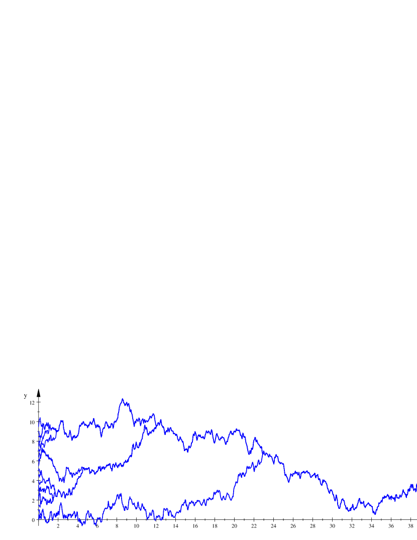
Figure 1: Point motion of the Arratia flow.

Roughly speaking, the Arratia flow consists of Brownian “particles” that evolve independently until they meet, and coalesce thereafter (Fig. 1). It is known that the $X\left(\cdot,t\right)$-image of any bounded subset of $\mathbb{R}$ is finite for any positive $t$ due to coalescence [3].

More generally, one can consider so-called Harris flows, defined the same way except that its “infinitesimal covariation function” may be an arbitrary real positive definite function:

$$\frac{d}{dt}\left\langle X\left(u,t\right),X\left(v,t\right)\right\rangle=\varphi\left(X\left(u,t\right)-X\left(v,t\right)\right).$$

We assume that $\varphi\left(0\right)=1$ for convenience. Furthermore, we assume that $\left|\varphi\left(x\right)\right|<1$ for $x\neq 0$, which excludes a possibility for periodic flows, regarded more naturally as flows on the circle. However, taking them into account would lead to no serious complications.

We study the asymptotical behaviour of

$$\sup_{u\in\left[0,1\right]}\left|X\left(u,t\right)-u\right|$$ (1)

for small $t$. The main approach is to compare $X\left(u,t\right)$ to a family of Gaussian martingales $\left(Y\left(u,t\right)\right)$ which we call a “tangent process”, defined by the following properties:

$$Y\left(u,0\right)=u,$$

$$\frac{d}{dt}\left\langle X\left(u,t\right),Y\left(v,t\right)\right\rangle=\varphi\left(X\left(u,t\right)-v\right),$$

$$\frac{d}{dt}\left\langle Y\left(u,t\right),Y\left(v,t\right)\right\rangle=\varphi\left(u-v\right).$$

Note that if $\varphi$ is continuous, then for any fixed $u$ the quadratic variation of $X\left(u,\cdot\right)-Y\left(u,\cdot\right)$ satisfies

$$\frac{d}{dt}\left\langle X\left(u,t\right)-Y\left(u,t\right)\right\rangle|_{t=0}=0.$$

Since $X\left(u,t\right)-Y\left(u,t\right)$ is a time-changed Brownian motion [6], one can easily deduce from the law of iterated logarithm that $\left|X\left(u,t\right)-Y\left(u,t\right)\right|=o\left(\sqrt{t\ln\ln t^{-1}}\right)$ as $t\to 0$. It turns out that if $Y$ has a modification that is continuous w.r.t. both variables then this holds uniformly in $u$. Namely,

$$\sup_{u\in\left[0,1\right]}\left|X\left(u,t\right)-Y\left(u,t\right)\right|=o\left(\sqrt{t\ln\ln t^{-1}}\right).$$

Together with the law of iterated logarithm for the Gaussian process $Y$ this yields

$$\limsup_{t\to 0}\frac{\sup_{u\in\left[0,1\right]}\left|X\left(u,t\right)-u\right|}{\sqrt{2t\ln\ln t^{-1}}}=1.$$

In Section 5 we consider the case when the “tangent process” has no continuous modification, which may happen if the covariation function is not smooth enough at zero. In this case we compare $X$ and $Y$ in distribution and obtain the following result:

$$\sup_{u\in\left[0,1\right]}\left|X\left(u,t\right)-u\right|-\mathsf{E}\sup_{0\leq k<t^{-1/2}}\left|Y\left(kt^{1/2},t\right)-kt^{1/2}\right|=O\left(\sqrt{t\ln\ln t^{-1}}\right).$$

The main tool used there is a martingale version of the Slepian comparison inequality, well-known in the theory of Gaussian processes [10]. The comparison inequality is stated and proved in Appendix (Theorem 9).

The paper is organized as follows. In Section 2 we give basic definitions and state an existence theorem for Harris flows. In Section 3 we give a universal $O\left(\sqrt{t\ln t^{-1}}\right)$ upper bound of (1) for monotone families of Brownian motions, which is used later. In Sections 4 and 5 we prove our main results for the flows with continuous and discontinuous tangent processes, respectively. In Appendix we prove the martingale comparison theorem and a classical result concerning concentration of measure that is needed in Section 5.

2 An existence result

Definition 1.

The point motion of a Harris flow is a family $\left(X\left(u,t\right)\right)_{u\in\mathbb{R},t\geq 0}$ of continuous martingales adapted to a common filtration $\left(\mathcal{F}_{t}\right)$, satisfying the following conditions:

1. For each $u$ $X\left(u,\cdot\right)$ is an $\mathcal{F}_{t}$-Brownian motion starting at $u$.

2. For each $u,v$ the joint covariation of $\left(X\left(u,\cdot\right)\right)$ and $\left(X\left(v,\cdot\right)\right)$ is given by

   $$\frac{d}{dt}\left\langle X\left(u,t\right),X\left(v,t\right)\right\rangle=\varphi\left(X\left(u,t\right)-X\left(v,t\right)\right),$$

   where $\left\langle\cdot,\cdot\right\rangle$ is quadratic covariation, and $\varphi$ is a positive definite function.

3. $\left(X\left(\cdot,t\right)\right)$ is monotone in $u$ for each $t$, and $\varphi$ is aperiodic.

Remark 2.

Note that condition 3 makes the Brownian motions coalesce once they hit each other.

Remark 3.

Once and for all, by $X$ we denote a modification that is separable and continuous in $t$ for each $u$.

The following existence resutlt is given in [5].

Theorem 4.

The Harris flow exists provided that $\varphi$ is Lipshitz outside each interval $\left(-c,c\right)$ and its spectral distribution is not of pure jump type.

In the sequel we will need not only $X$ itself, but also a Gaussian process $\left(Y\left(u,t\right)\right)$ starting at $u$ with joint covariation given below:

$$\frac{d}{dt}\left\langle Y\left(u,t\right),Y\left(v,t\right)\right\rangle=\varphi\left(u-v\right),$$

$$\frac{d}{dt}\left\langle X\left(u,t\right),Y\left(v,t\right)\right\rangle=\varphi\left(X\left(u,t\right)-v\right).$$ (2)

It admits a construction of the following kind:

$$Y\left(u,t\right)=u+\sum_{i}\intop_{0}^{t}a_{i}\left(u,s\right)dX\left(v_{i},s\right)+\sum_{j}\intop_{0}^{t}b_{j}\left(u,s\right)dW_{j}\left(s\right),$$

where $\left\{v_{i}\right\}$ is a countable dense subset of $\mathbb{R}$, $W_{j}$ are independent Brownian motions that are also independent of $X$, $a$ and $b$ are adapted to the filtration generated by $X$ and $W$. It is easy to show that $a_{i}$ and $b_{j}$ can be chosen in such a way that the covariation satisfies (2). However, it is not unique, since the construction involves additional randomization.

3 An upper bound

An important special case of a Harris flow is the Arratia flow (Fig. 1). Its covariation function $\varphi$ is given by $\varphi\left(0\right)=1$ and $\varphi=0$ elsewhere. Thus the “particles” $X\left(u,\cdot\right)$ move independently until they coalesce. It follows from our results that the point motion of the Arratia flow has the following asymptotics in the $\sup$-norm:

$$\sup_{u\in\left[0,1\right]}\left|X\left(u,t\right)-u\right|\sim\sqrt{t\ln t^{-1}},t\to 0.$$ (3)

Now we will see that the Arratia flow is in some sense the “extreme case”. Namely, for any Harris flow (and in fact for any monotone family of Brownian motions) an inequality in (3) holds.

Theorem 5.

For any Harris flow $X$ with $\varphi\left(0\right)=1$ one has

$$\limsup_{t\to 0}\sup_{u\in\left[0,1\right]}\frac{\left|X\left(u,t\right)-u\right|}{\sqrt{t\ln t^{-1}}}\leq 1.$$

Proof.

First let’s prove the inequality for an increasing number of points $u_{nk}=kt_{n}^{1/2}$, where $t_{n}=q^{n},0<q<1$.

$$\sum_{n}\mathsf{P}\left\{\sup_{0\leq k\leq t_{n}^{-1/2}}\sup_{s\leq t_{n}}\left|X\left(u_{nk},s\right)-u_{nk}\right|\geq\sqrt{\left(1+\varepsilon\right)t_{n}\ln t_{n}^{-1}}\right\}\leq\\ \leq\sum_{n}\left\lceil t_{n}^{-1/2}\right\rceil\mathsf{P}\left\{\sup_{s\leq t_{n}}\left|X\left(u_{n0},s\right)-u_{n0}\right|\geq\sqrt{\left(1+\varepsilon\right)t_{n}\ln t_{n}^{-1}}\right\}\leq\\ \leq\mathrm{const}\cdot\sum_{n}t_{n}^{-1/2}\exp\left[-\frac{1}{2}\left(1+\varepsilon\right)\ln t_{n}^{-1}\right]=\mathrm{const}\cdot\sum_{n}q^{n\varepsilon/2}<+\infty.$$

The Borel-Cantelli lemma implies

$$\limsup_{n\to\infty}\sup_{k}\sup_{s\leq t_{n}}\frac{\left|X\left(u_{nk},s\right)-u_{nk}\right|}{\sqrt{t_{n}\ln t_{n}^{-1}}}\leq 1.$$

Now let $u$ be an arbitrary point from $\left[0,1\right]$, and let $k$ be such that $u_{nk}\leq u\leq u_{n,k+1}$ for a fixed $t_{n}$. Using the monotonicity property, we obtain

$$\left|X\left(u,s\right)-u\right|\leq\left|X\left(u_{nk},s\right)-u\right|\vee\left|X\left(u_{n,k+1},s\right)-u\right|\leq\\ \leq\left|X\left(u_{nk},s\right)-u_{nk}\right|\vee\left|X\left(u_{n,k+1},s\right)-u_{n,k+1}\right|+\sqrt{t_{n}}.$$

Thus,

$$\limsup_{n\to\infty}\sup_{u\in\left[0,1\right]}\sup_{s\leq t_{n}}\frac{\left|X\left(u,s\right)-u\right|}{\sqrt{t_{n}\ln t_{n}^{-1}}}\leq 1.$$

Now by taking $q$ close enough to $1$ we prove the statement. The argument is basically the same as in the proof of the law of iterated logarithm. Namely, let $q$ be such that $\sqrt{q^{n}\ln q^{-n}}\geq\left(1+\varepsilon\right)\sqrt{q^{n+1}\ln q^{-n-1}}$ for sufficiently large $n$. Then since $\sqrt{t\ln t^{-1}}$ is monotone for small $t$, we obtain

$$\limsup_{t\to 0}\sup_{u\in\left[0,1\right]}\frac{\left|X\left(u,t\right)-u\right|}{\sqrt{t\ln t^{-1}}}\leq\left(1+\varepsilon\right)\limsup_{t\to 0}\sup_{u\in\left[0,1\right]}\frac{\left|X\left(u,t\right)-u\right|}{\sqrt{t_{n}\ln t_{n}^{-1}}}\leq 1+\varepsilon,$$

where $t_{n}=q^{n}$ is such that $q^{n+1}\leq t\leq q^{n}$. ∎

4 The continuous case

In this paper we estimate the asymptotics of $X$ by comparing it to the process which we denote $Y$, defined by (2). It is a Gaussian process, stationary in $u\in\mathbb{R}$, and also a Brownian motion in $t$, in the sense that its increments are stationary and independent. In this section we consider the case when it has a continuous modification. Note that continuity w.r.t. both variables follows easily from continuity of $Y\left(\cdot,1\right)$. Indeed, when restricted to $u\in\left[0,1\right]$ the process becomes a $C\left[0,1\right]$-valued Brownian motion for which Kolmogorov’s continuity criterion is applicable.

A well-known result of the theory of Gaussian processes states that a stationary Gaussian process has a continuous (or, equivalently, bounded) modification iff its Dudley integral converges [10]. In our case this is equivalent to

$$\intop_{0+}\left|\ln\lambda\left\{x\,\middle|\,\varphi\left(x\right)\geq 1-u^{2}\right\}\right|^{1/2}du<+\infty,$$ (4)

where $\lambda$ is the Lebesgue measure on $\left[0,1\right]$. Note that continuity of $Y$ does not imply continuity of $X$ . Nevertheless, the following result shows that $X$ is close to $Y$ in the $\sup$-norm.

Theorem 6.

Assuming that $Y$ has a continuous modification,

$$\sup_{u\in\left[0,1\right]}\left|X\left(u,t\right)-Y\left(u,t\right)\right|=o\left(\sqrt{t\ln\ln t^{-1}}\right).$$

Proof.

Take a function $\alpha:\left[0,1\right]\to\mathbb{R}_{+}$ that is monotone, continuous, satisfying $\alpha\left(0\right)=0$ and such that

$$\left\|Y\left(\cdot,1\right)\right\|_{\alpha}:=\sup_{0\leq u<v\leq 1}\frac{\left|Y\left(u,1\right)-Y\left(v,1\right)\right|}{\alpha\left(\left|u-v\right|\right)}<+\infty\text{ a.s.}$$ (5)

Its existence may be easily deduced from the fact that the distribution of $Y\left(\cdot,1\right)$ is supported on a $\sigma$-compact subspace of $C\left[0,1\right]$. Let $t_{n}$ be $q^{n}$ for some $0<q<1$, and let’s consider $\left\lfloor\ln n\right\rfloor$ points $u_{nk}:=k/\ln n$. For $Y$ to have a continuous modification, $\varphi$ must be continuous at zero. Therefore, $X\left(u,\cdot\right)-Y\left(u,\cdot\right)$ are martingales whose quadratic variation is $o\left(t\right)$ uniformly in $u$:

$$V\left(t\right):=\sup_{u\in\left[0,1\right]}\left|\left\langle X\left(u,t\right)-Y\left(u,t\right)\right\rangle\right|=2\sup_{u\in\left[0,1\right]}\left|\intop_{0}^{t}\left(1-\varphi\left(X\left(u,s\right)-u\right)\right)ds\right|=o\left(t\right).$$ (6)

This implies that $\left|X\left(u,t\right)-Y\left(u,t\right)\right|$ must be $o\left(\sqrt{t\ln\ln t^{-1}}\right)$ for each $u$, and moreover, uniformly in $u=u_{nk}$, since there are “not too many” of them. More precisely, let $\tau$ be $\inf\left\{t\,\middle|\,V\left(t\right)>\varepsilon t\right\}$. One-dimensional continuous martingales are time-changed Brownian motions [6], hence

$$\sum_{n}\mathsf{P}\left\{\sup_{0\leq k<1/\ln n}\sup_{s\leq t_{n}}\left|X\left(u_{nk},s\wedge\tau\right)-Y\left(u_{nk},s\wedge\tau\right)\right|\geq\sqrt{3\varepsilon t_{n}\ln\ln t_{n}^{-1}}\right\}\leq\\ \leq\mathrm{const}\cdot\sum_{n}\ln n\cdot\exp\left[-\frac{1}{2}\cdot 3\ln\ln t_{n}^{-1}\right]\leq\mathrm{const}\cdot\sum_{n}\ln n\cdot\left(\ln t_{n}^{-1}\right)^{-3/2}=\\ =\mathrm{const}\cdot\sum_{n}\frac{\ln n}{n^{3/2}}<+\infty.$$

By letting $\varepsilon$ be small enough we obtain

$$\sup_{k}\sup_{s\leq t_{n}}\left|X\left(u_{nk},s\wedge\tau\right)-Y\left(u_{nk},s\wedge\tau\right)\right|=o\left(\sqrt{t_{n}\ln\ln t_{n}^{-1}}\right).$$

Since $\tau$ is a.s. positive, we may use $X\left(u_{nk},s\right)-Y\left(u_{nk},s\right)$ instead of $X\left(u_{nk},s\wedge\tau\right)-Y\left(u_{nk},s\wedge\tau\right)$.

Points $u\in\left[0,1\right]$ other than $u_{nk}$ may be treated as follows. Let $k$ be such that $u_{nk}\leq u\leq u_{n,k+1}$. Then

$$\left|X\left(u,s\right)-Y\left(u,s\right)\right|\leq\\ \leq 2\left|Y\left(u_{nk},s\right)-X\left(u_{nk},s\right)\right|+\left|Y\left(u_{n,k+1},s\right)-X\left(u_{n,k+1},s\right)\right|+\\ +\left|Y\left(u_{n,k+1},s\right)-Y\left(u_{nk},s\right)\right|+\left|Y\left(u,s\right)-Y\left(u_{nk},s\right)\right|,s\leq t_{n}.$$ (7)

The first two terms in (7) are already shown to be uniformly $o\left(\sqrt{t_{n}\ln\ln t_{n}^{-1}}\right)$. The last two terms are actually $O\left(\alpha\left(u_{n,k+1}-u_{nk}\right)\sqrt{t_{n}\ln\ln t_{n}^{-1}}\right)$ uniformly in $k$ and $s\leq t_{n}$. This follows from the concentration principle for the $\alpha$-seminorm in (5), which is in fact valid for any Lipshitz function of a Gaussian random vector (see Theorem 17 in Appendix). More precisely, the following inequality holds:

$$\mathsf{P}\left\{\left\|Y\left(\cdot,t\right)\right\|_{\alpha}\geq\mathsf{E}\left\|Y\left(\cdot,t\right)\right\|_{\alpha}+C\right\}\leq e^{-C^{2}/2\sigma^{2}t}.$$

for some $\sigma$ and any positive $C$. Together with the fact that $\mathsf{E}\left\|Y\left(\cdot,t\right)\right\|_{\alpha}$ is finite and evidently $O\left(t\right)$, this yields

$$\left\|Y\left(\cdot,t_{n}\right)\right\|_{\alpha}=O\left(\sqrt{t_{n}\ln\ln t_{n}^{-1}}\right).$$

Therefore,

$$\sup_{s\leq t_{n}}\left|X\left(u,s\right)-Y\left(u,s\right)\right|\leq o\left(\sqrt{t_{n}\ln\ln t_{n}^{-1}}\right)+\alpha\left(1/\ln t_{n}\right)\left\|Y\left(\cdot,t_{n}\right)\right\|_{\alpha}=\\ =o\left(\sqrt{t_{n}\ln\ln t_{n}^{-1}}\right).$$

$t\neq t_{n}$ are handled in a usual way by letting $q$ close to $1$. ∎

Though there are cases when the “tangent process” is discontinuous and nevertheless the difference $X-Y$ is small enough, it seems that this is not the case in general. That’s why in the sequel we do not estimate the difference but rather compare the tail probabilities of $X$ with those of $Y$. In this way we estimate $\sup_{u\in\left[0,1\right]}\left|X\left(u,t\right)-u\right|$ up to an $O\left(\sqrt{t\ln\ln t^{-1}}\right)$ term, which is slightly weaker than the $o\left(\sqrt{t\ln\ln t^{-1}}\right)$ in Theorem 6.

5 Tail comparison

In this section we consider short-time asymptotical behaviour of the flow with no regularity assumptions on the “tangent process” except local monotonicity of the covariation function. Basically, we use the same approach as in Theorems 5 and 6. Namely, we start by estimating the deviation of an increasing number of points $u_{nk}$, and then use the monotonicity property of the flow to handle the points other than $u_{nk}$. It turns out that $t_{n}^{-1/2}$ points $u_{nk}=kt_{n}^{1/2}$ give the right asymptotics up to an $O\left(\sqrt{t_{n}\ln\ln t_{n}^{-1}}\right)$ term.

As it was mentioned earlier, we compare the asymptotical behavior of the flow to that of a Gaussian process. So first of all, let’s see what happens in the Gaussian case. It is known that the probability distribution of the supremum of a Gaussian process is concentrated around its mean at least as strongly as a single Gaussian r.v. is (see Theorem 17 in Appendix). That is, if $M$ is a centered Gaussian vector in $\mathbb{R}^{d}$, then

$$\mathsf{P}\left\{\left|\sup_{i}M^{i}-\mathsf{E}\sup_{i}M^{i}\right|\geq x\right\}\leq Ce^{-x^{2}/2\sigma^{2}}.$$ (8)

for some absolute constant $C$ and any $x\geq 0$, $\sigma^{2}$ being $\sup_{i}\mathsf{E}\left(M^{i}\right)^{2}$. From this concentration inequality it is easy to deduce a law of iterated logarithm of the following kind:

$$\limsup_{n\to+\infty}\frac{\left|\sup_{k}\left|Y\left(u_{nk},t_{n}\right)-u_{nk}\right|-\mathsf{E}\sup_{k}\left|Y\left(u_{nk},t_{n}\right)-u_{nk}\right|\right|}{\sqrt{2t_{n}\ln\ln t_{n}^{-1}}}\leq 1.$$

If $Y$ is continuous, then $\mathsf{E}\sup_{k}\left|Y\left(u_{nk},t_{n}\right)-u_{nk}\right|\sim\mathrm{const}\cdot t_{n}^{1/2}$. In our case, though, the process may be discontinuous, and $\mathsf{E}\sup_{k}\left|Y\left(u_{nk},t_{n}\right)-u_{nk}\right|$ may be asymptotically greater than $\sqrt{t_{n}\ln\ln t_{n}^{-1}}$. Actually, for the Arratia flow $Y$ consists of independent Brownian motions, and in this case

$$\sup_{k}\left|Y\left(u_{nk},t_{n}\right)-u_{nk}\right|\sim\mathsf{E}\sup_{k}\left|Y\left(u_{nk},t_{n}\right)-u_{nk}\right|\sim\sqrt{t_{n}\ln t_{n}^{-1}}.$$

We do not know whether a concentration inequality similar to (8) holds for $\sup_{u}\left|X\left(u,t\right)-u\right|$. Nevertheless, we show that $\sup_{u}\left|X\left(u,t\right)-u\right|$ is deterministic up to $O\left(\sqrt{t\ln\ln t^{-1}}\right)$.

Theorem 7.

Assume that $\varphi$ is monotone on $\left[0,\delta\right]$ for some $\delta>0$. Then

$$\sup_{u\in\left[0,1\right]}\left|X\left(u,t\right)-u\right|=E\left(t\right)+O\left(\sqrt{t\ln\ln t^{-1}}\right),t\to 0\text{ a.s.},$$ (9)

$E\left(t\right)$ being defined by

$$E\left(t\right)=\mathsf{E}\sup_{0\leq k<t^{-1/2}}\left|Y\left(kt^{1/2},t\right)-kt^{1/2}\right|.$$

Proof.

In the proof we assume that $\varphi$ is monotone on $\left(0,+\infty\right)$. If $\varphi$ is only locally monotone, the result is obtained for sufficiently small intervals instead of $\left[0,1\right]$.

First let’s prove the upper bound. As usual, take $t_{n}=q^{n}$ and $u_{nk}=kt_{n}^{1/2}$. For the comparison inequality (Theorem 9) to be applicable we need a deterministic bound from below on the infinitesimal covariation of the martingale $\left(X\left(u_{nk},t\right)-u_{nk}\right)$. If $\varphi$ is monotone on $\left[0,+\infty\right)$, it is sufficient to obtain a deterministic upper bound on $\sup_{t\leq t_{n}}\sup_{k}\left|X\left(u_{nk},t\right)-u_{nk}\right|$. So we stop the martingale once the deviation gets too large. To be precise, let’s consider the following optional times:

$$\tau_{n}:=\inf\left\{t\,\middle|\,\sup_{u\in\left[0,1\right]}\left|X\left(u,t\right)-u\right|\geq 2\sqrt{t_{n}\ln t_{n}^{-1}}\right\}.$$

Theorem 5 implies that a.s. $\tau_{n}\geq t_{n}$ for sufficiently large $n$. Take $\tilde{u}_{nk}:=2\left\lceil\sqrt{\ln t_{n}^{-1}}\right\rceil u_{nk}$. If $\varphi$ is monotone on $\left[0,+\infty\right)$, then the $2\left\lfloor t_{n}^{-1/2}\right\rfloor$-dimensional martingales $\pm\left(X\left(u_{nk},t\wedge\tau_{n}\right)-u_{nk}\right)$ and $\pm\left(Y\left(\tilde{u}_{nk},t\right)-\tilde{u}_{nk}\right)$ satisfy the conditions of Theorem 9. Thus

$$\mathsf{E}\exp\lambda\sup_{k}\left|X\left(u_{nk},t_{n}\wedge\tau_{n}\right)-u_{nk}\right|\leq\mathsf{E}\exp\lambda\sup_{k}\left|Y\left(\tilde{u}_{nk},t_{n}\right)-\tilde{u}_{nk}\right|$$

for any $\lambda\geq 0$ (see also Remark 10 in Appendix). Since $\sup_{k}\left|X\left(u_{nk},t\wedge\tau_{n}\right)-u_{nk}\right|$ is a submartingale, the well-known (sub)martingale inequalities [6] imply

$$\mathsf{E}\exp\lambda\sup_{t\leq t_{n}}\sup_{k}\left|X\left(u_{nk},t\wedge\tau_{n}\right)-u_{nk}\right|\leq\mathrm{const}\cdot\mathsf{E}\exp\lambda\sup_{k}\left|Y\left(\tilde{u}_{nk},t_{n}\right)-\tilde{u}_{nk}\right|.$$ (10)

The right-hand term may be estimated by means of the concentration inequality (Theorem 17):

$$\mathsf{E}\exp\lambda\sup_{k}\left|Y\left(\tilde{u}_{nk},t_{n}\right)-\tilde{u}_{nk}\right|\leq\exp\left[\lambda\mathsf{E}\sup_{k}\left|Y\left(\tilde{u}_{nk},t_{n}\right)-\tilde{u}_{nk}\right|+t_{n}\lambda^{2}/2\right].$$ (11)

What remains is to show that

$$\mathsf{E}\sup_{k}\left|Y\left(\tilde{u}_{nk},t_{n}\right)-\tilde{u}_{nk}\right|=E\left(t_{n}\right)+O\left(\sqrt{t_{n}\ln\ln t_{n}^{-1}}\right),$$

that is, to compare $\mathsf{E}\sup_{k}\left|Y\left(Nu_{nk},t_{n}\right)-Nu_{nk}\right|$ and $\mathsf{E}\sup_{k}\left|Y\left(u_{nk},t_{n}\right)-u_{nk}\right|$, $N$ being equal to $2\left\lceil\sqrt{\ln t_{n}^{-1}}\right\rceil$. The following inequality is trivial:

$$\sup_{0\leq k<t_{n}^{-1/2}}\left|Y\left(Nu_{nk},t_{n}\right)-Nu_{nk}\right|\leq\sup_{0\leq m<C}S_{m},$$

where

$$S_{m}:=\sup_{0\leq k<t_{n}^{-1/2}}\left|Y\left(u_{nk}+mt_{n}^{1/2},t_{n}\right)-u_{nk}-mt_{n}^{1/2}\right|.$$

Note that $S_{m}$ are identically distributed, and also sub-Gaussian due to the concentration inequality. That is,

$$\mathsf{E}\exp\lambda S_{m}\leq\exp\left(\lambda\mathsf{E}S_{m}+t_{n}\lambda^{2}/2\right).$$

What follows is a classical argument that gives an upper bound for the expectation of supremum of independent sub-Gaussian variables [10].

$$\mathsf{E}\sup_{m}S_{m}\leq\inf_{\lambda}\frac{1}{\lambda}\ln\mathsf{E}\exp\lambda\sup_{m}S_{m}\leq\inf_{\lambda}\frac{1}{\lambda}\ln\sum_{m}\mathsf{E}\exp\lambda S_{m}\leq\\ \leq\inf_{\lambda}\frac{1}{\lambda}\ln\left(N\exp\left(\lambda\mathsf{E}S_{m}+t_{n}\lambda^{2}/2\right)\right)=\inf_{\lambda}\left(\mathsf{E}S_{m}+t_{n}\lambda/2+\frac{\ln N}{\lambda}\right)=\\ =\mathsf{E}S_{m}+\sqrt{2t_{n}\ln N}.$$

Since $N\asymp\sqrt{\ln t_{n}^{-1/2}}$, we obtain

$$\mathsf{E}\sup_{k}\left|Y\left(\tilde{u}_{nk},t_{n}\right)-\tilde{u}_{nk}\right|\leq E\left(t_{n}\right)+O\left(\sqrt{t_{n}\ln\ln t_{n}^{-1}}\right).$$ (12)

By combining (10), (11) and (12), we obtain

$$\mathsf{E}\exp\lambda\sup_{t\leq t_{n}}\sup_{k}\left|X\left(u_{nk},t\wedge\tau_{n}\right)-u_{nk}\right|\leq\\ \leq\mathrm{const}\cdot\exp\left[\lambda\left(E\left(t_{n}\right)+\mathrm{const}\cdot\sqrt{t_{n}\ln\ln t_{n}^{-1}}\right)+t_{n}\lambda^{2}/2\right].$$

Now to estimate the tail probability we may use the Chernoff bound [11]:

$$\mathsf{P}\left\{\sup_{t\leq t_{n}}\sup_{k}\left|X\left(u_{nk},t\wedge\tau_{n}\right)-u_{nk}\right|\geq C+E\left(t_{n}\right)+\mathrm{const}\cdot\sqrt{t_{n}\ln\ln t_{n}^{-1}}\right\}\leq\\ \leq\mathrm{const}\cdot\inf_{\lambda}e^{-\lambda C+t_{n}\lambda^{2}/2}=\mathrm{const}\cdot e^{-C^{2}/2t_{n}}.$$

This implies the upper bound in the law of iterated logarithm for

$$\sup_{t\leq t_{n}}\sup_{k}\left|X\left(u_{nk},t\wedge\tau_{n}\right)-u_{nk}\right|-E\left(t_{n}\right),$$

and since $\tau_{n}\geq t_{n}$ for $n$ sufficiently large, the same for

$$\sup_{t\leq t_{n}}\sup_{k}\left|X\left(u_{nk},t\right)-u_{nk}\right|-E\left(t_{n}\right).$$

The remaining steps are routine.

The lower bound in (9) is obtained along the same way. The difference is that now we exchange $u_{nk}$ and $\tilde{u}_{nk}$ to get a bound on the infinitesimal covariation from below. ∎

6 Appendix: Comparison and Concentration

The classical comparison inequality due to Slepian says that if $\left(M^{i}\right)$ and $\left(N^{i}\right)$ are centered Gaussian random vectors in $\mathbb{R}^{d}$ with $\mathsf{E}\left(M^{i}\right)^{2}=\mathsf{E}\left(N^{i}\right)^{2}$ and $\mathsf{E}M^{i}M^{j}\geq\mathsf{E}N^{i}N^{j}$, then $\max_{i}N^{i}$ stochastically dominates $\max_{i}M^{i}$ [10]. For our purpose we need a generalization involving martingales compared by quadratic covariation instead of Gaussian vectors compared by covariance.

We start with a martingale version of the lemma that is used to derive comparison inequalities for Gaussian vectors [10].

Lemma 8.

Let $\left(M\left(t\right)\right)_{t\in\left[0,1\right]}$ be a continuous $\mathbb{R}^{d}$-valued martingale and $\left(N\left(t\right)\right)_{t\in\left[0,1\right]}$ be a continuous $\mathbb{R}^{d}$-valued Gaussian martingale, both with absolutely continuous quadratic variation and satisfying $M\left(0\right)=N\left(0\right)=0$. Assume that $N$ is independent of $M$. Then for any $C^{2}$-smooth function $f:\mathbb{R}^{d}\to\mathbb{R}$ with second derivatives of at most exponential growth the following equality holds:

$$\mathsf{E}f\left(M\left(1\right)\right)-\mathsf{E}f\left(N\left(1\right)\right)=\\ =\frac{1}{2}\intop_{0}^{1}\sum_{i,j}\mathsf{E}\partial_{ij}f\left(M\left(t\right)+N\left(1\right)-N\left(t\right)\right)\left(K_{M}^{ij}\left(t\right)-K_{N}^{ij}\left(t\right)\right)dt,$$ (13)

where

$$K_{M}^{ij}\left(t\right)=\frac{d}{dt}\left\langle M^{i}\left(t\right),M^{j}\left(t\right)\right\rangle,$$

$$K_{N}^{ij}\left(t\right)=\frac{d}{dt}\left\langle N^{i}\left(t\right),N^{j}\left(t\right)\right\rangle.$$

Proof.

Let’s denote $N\left(1\right)-N\left(1-t\right)$ by $\tilde{N}\left(t\right)$. Since $N$ is a Gaussian martingale, $\tilde{N}$ is a Gaussian martingale as well. We may assume that $M$ and $\tilde{N}$ are adapted to independent filtrations $\left(\mathcal{F}_{t}\right)$ and $\left(\mathcal{G}_{t}\right)$, respectively. Consider a two-parametric process

$$F\left(t,s\right):=f\left(M\left(t\right)+\tilde{N}\left(s\right)\right).$$

Using Itô’s formula w.r.t. $t$ and $s$ separately and taking expectations, we obtain:

$$\frac{\partial}{\partial t}\mathsf{E}F\left(t,s\right)=\frac{1}{2}\sum_{i,j}\mathsf{E}\partial_{ij}f\left(M\left(t\right)+\tilde{N}\left(s\right)\right)K_{M}^{ij}\left(t\right),$$

$$\frac{\partial}{\partial s}\mathsf{E}F\left(t,s\right)=\frac{1}{2}\sum_{i,j}\mathsf{E}\partial_{ij}f\left(M\left(t\right)+\tilde{N}\left(s\right)\right)K_{N}^{ij}\left(1-s\right).$$

Therefore,

$$\frac{\partial}{\partial t}\mathsf{E}F\left(t,1-t\right)=\frac{1}{2}\sum_{i,j}\mathsf{E}\partial_{ij}f\left(M\left(t\right)+\tilde{N}\left(1-t\right)\right)\left(K_{M}^{ij}\left(t\right)-K_{N}^{ij}\left(t\right)\right).$$

Finally, by integrating over $t\in\left[0,1\right]$ we finish the proof. ∎

Now suppose that we are given an inequality between $K_{M}^{ij}$ and $K_{N}^{ij}$. It is then clear that by means of Lemma 8 we may obtain an inequality between $\mathsf{E}f\left(M\left(1\right)\right)$ and $\mathsf{E}f\left(N\left(1\right)\right)$ for an appropriate class of functions.

Theorem 9 (Martingale comparison).

Let $M$ and $N$ be a martingale and a Gaussian martingale with absolutely continuous quadratic variation, and let $f:\mathbb{R}^{d}\to\mathbb{R}$ be a Borel function of at most exponential growth. Assume that the following inequalities hold:

$$K_{M}^{ii}+K_{M}^{jj}-2K_{M}^{ij}\leq K_{N}^{ii}+K_{N}^{jj}-2K_{N}^{ij},i\neq j,$$

$$K_{M}^{ii}\leq K_{N}^{ii},$$

$$\partial_{ij}f\leq 0,i\neq j.$$ (14)

Furthermore, assume that either one of the following additional conditions is fulfilled:

1. $$K_{M}^{ii}=K_{N}^{ii}$$

2. $$\sum_{j}\partial_{ij}f\geq 0\text{ for each }i$$ (15)

Then

$$\mathsf{E}f\left(M\left(1\right)\right)\leq\mathsf{E}f\left(N\left(1\right)\right).$$

Proof.

Assume that the second derivatives of $f$ are continuous and of at most exponential growth. Then by Lemma 8 we have

$$\mathsf{E}f\left(M\left(1\right)\right)-\mathsf{E}f\left(N\left(1\right)\right)=\frac{1}{2}\intop_{0}^{1}\sum_{i,j}\mathsf{E}\partial_{ij}f\left(M\left(t\right)+N\left(1\right)-N\left(t\right)\right)\left(K_{M}^{ij}-K_{N}^{ij}\right)dt.$$

Note that in order to use Lemma 8 we assume that $M$ and $N$ are independent. If they are not, we may replace $N$ by an independent process with the same distribution.

Next we rewrite the right-hand side in the following way:

$$\sum_{i,j}\partial_{ij}f\cdot\left(K_{M}^{ij}-K_{N}^{ij}\right)=\\ =\sum_{i<j}\partial_{ij}f\cdot\left[\left(2K_{M}^{ij}-K_{M}^{ii}-K_{M}^{jj}\right)-\left(2K_{N}^{ij}-K_{N}^{ii}-K_{N}^{jj}\right)\right]+\\ +\sum_{i}\left(\sum_{j}\partial_{ij}f\right)\left(K_{M}^{ii}-K_{N}^{ii}\right).$$

The conditions imposed upon $f$ and $K_{M}-K_{N}$ ensure that each term is negative.

The case when $f$ is not smooth enough may be treated by means of an approximation argument. Namely, let $\varphi_{\varepsilon}\in C^{\infty}\left(\mathbb{R}^{d}\to\mathbb{R}\right)$ be a nonnegative function supported on $\left\{\left\|x\right\|\leq\varepsilon\right\}$, such that $\intop\varphi_{\varepsilon}dx=1$. Then $f\ast\varphi_{\varepsilon}$ satisfies the conditions of Lemma 8, and $f\ast\varphi_{\varepsilon}$ converges to $f$ in $L^{1}$ over any Gaussian measure due to the growth condition.∎

Remark 10.

The basic condition (14) is referred to as submodularity or $L$-subadditivity. It is known to be equivalent to the following inequality that involves only the lattice structure:

$$f\left(x\wedge y\right)+f\left(x\vee y\right)\leq f\left(x\right)+f\left(y\right)\text{ for all }x,y\in\mathbb{R}^{d}.$$

Here $x\wedge y$ and $x\vee y$ are coordinatewise minimum and maximum, respectively. Examples of submodular functions include $f\left(x^{1},\dots,x^{d}\right)=\varphi\left(\max_{i}x^{i}\right)$ for any increasing function $\varphi$. If $\varphi$ is also convex, then $f$ satisfies (15).

Remark 11.

It is clear that $M$ and $N$ may be exchanged, as long as integrability issues are taken care of. Thus we also have comparison inequalities in the case when the infinitesimal covariation of a martingale is bounded deterministically from below.

Next we present the basic result concerning concentration of measure for Lipshitz functionals of Gaussian random vectors. What follows is a short proof based on martingale comparison [9]. Another approach based on the isoperimetric properties of Gaussian measures may be found in [9, 10].

Theorem 12 (The concentration principle).

Let $N$ be a standard Gaussian random vector in $\mathbb{R}^{d}$, and let $f$ be a Lipshitz function with Lipshitz constant $L$. Then the following inequalities hold:

$$\mathsf{E}\exp\lambda\left(f\left(N\right)-\mathsf{E}f\left(N\right)\right)\leq\exp\left(\lambda^{2}L^{2}/2\right),\forall\lambda\in\mathbb{R},$$ (16)

$$\mathsf{P}\left\{f\left(N\right)-\mathsf{E}f\left(N\right)\geq C\right\}\leq\exp\left(-C^{2}/2L^{2}\right),\forall C\geq 0.$$ (17)

Proof.

Let $\left(N\left(t\right),0\leq t\leq 1\right)$ be a standard Brownian motion in $\mathbb{R}^{d}$ with $N=N\left(1\right)$. Denote by $\mathcal{F}_{t}$ the induced filtration. We consider the martingale

$$\Phi\left(t\right):=\mathsf{E}\left[f\left(N\right)\,\middle|\,\mathcal{F}_{t}\right]$$

and intend to prove that

$$d\left\langle\Phi,\Phi\right\rangle\leq L^{2}dt.$$ (18)

By an application of Theorem 9 to $\Phi-\mathsf{E}f\left(N\right)$ and the Brownian motion in $\mathbb{R}$ with quadratic variation $L^{2}t$, this would imply (16). To bound the tail probability in (17) we may then use the classical Chernoff bound [11]:

$$\mathsf{P}\left\{f\left(N\right)-\mathsf{E}f\left(N\right)\geq C\right\}\leq\inf_{\lambda\geq 0}e^{-\lambda C}\mathsf{E}\exp\lambda\left(f\left(N\right)-\mathsf{E}f\left(N\right)\right)\leq\\ \leq\inf_{\lambda\geq 0}\exp\left(-\lambda C+\lambda^{2}L^{2}/2\right)=\exp\left(-C^{2}/2L^{2}\right).$$

What remains is to prove (18). For this we note that

$$\mathsf{E}\left[f\left(N\left(1\right)\right)\,\middle|\,\mathcal{F}_{t}\right]=\mathsf{E}\left[f\left(N\left(1\right)\right)\,\middle|\,N\left(t\right)\right]=T^{1-t}f\left(N\left(t\right)\right),$$

where $T$ is the Brownian semigroup. The stochastic differential $dT^{1-t}f\left(N\left(t\right)\right)$ can be calculated using Itô’s formula. Note that the $dt$ terms vanish automatically since $\Phi$ is a martingale, and just the $dN$ term remains:

$$dT^{1-t}f\left(N\left(t\right)\right)=\sum_{i}T^{1-t}\partial_{i}f\left(N\left(t\right)\right)dN^{i}\left(t\right).$$

Now the Lipshitz condition implies (18).∎

Remark 13.

Of course, Theorem 17 may be formulated for any Gaussian random vector, not just a standard one. In this case the Lipshitz condition is assumed w.r.t. the Euclidean metric induced by the Gaussian measure.

References

- [1] R.A. Arratia, Coalescing Brownian motions and the voter model on , U.S.C. Preprint, 1985
- [2] R.W.R. Darling, Constructing nonhomeomorphic stochastic flows, IMA, Univ. of Minnesota, 1985
- [3] A.A. Dorogovtsev, Measure-valued processes and stochastic flows, Inst. of Math., Kiev, 2007 (in Russian)
- [4] L.R.G. Fontes, M. Isopi, C.M. Newman, K. Ravishankar, The Brownian Web — characterization and convergence, arXiv:math.PR/0304119
- [5] T.E. Harris, Coalescing and noncoalescing stochastic flows in , Stoch. Proc. Appl. 17, pp. 187-210, 1984
- [6] O. Kallenberg, Foundations of Modern Probability, Springer, 1997
- [7] H. Kunita, Stochastic flows and stochastic differential equations, Cambridge Univ. Press, 1990
- [8] Y. Le Jan, O. Raimond, Flows, Coalescence and Noise, arXiv:math.PR/0203221, Ann. of Prob. 32:2, pp. 1247-1315, 2004
- [9] M. Ledoux, Isoperimetry and Gaussian analysis, École d’Été de Probabilités de Saint-Flour, 1994
- [10] M. Lifshits, Gaussian random functions, Kluwer, 1995
- [11] G. Lugosi, Concentration-of-measure inequalities, 2006
- [12] H. Matsumoto, Coalescing stochastic flows on the real line, Osaka J. Math. 26, pp. 139-158, 1989
- [13] A. Maurer, A proof of Slepian’s inequality, www.andreas-maurer.eu/Slepian3.pdf