Density profiles of loose and collapsed cohesive granular structures generated by ballistic deposition

Abstract

Loose granular structures stabilized against gravity by an effective cohesive force are investigated on a microscopic basis using contact dynamics. We study the influence of the granular Bond number on the density profiles and the generation process of packings, generated by ballistic deposition under gravity. The internal compaction occurs discontinuously in small avalanches and we study their size distribution. We also develop a model explaining the final density profiles based on insight about the collapse of a packing under changes of the Bond number.

I Introduction

Loose granular packings, metastable granular structures and fragile granular networks play an important role in a wide range of scientific disciplines, such as collapsing soils Mitchell and Soga (2005); Barden et al. (1973); Assallay et al. (1997); Reznik (2005), fine powders Rognon et al. (2006a) or complex fluids Wagner and Brady (2009); Gado and Kob (2010). In collapsing soils without any doubt there is a metastable or fragile granular network involved Mitchell and Soga (2005); Barden et al. (1973); Assallay et al. (1997); Kadau et al. (2009a, b). A similar failure behavior can be found in colloidal gels Manley et al. (2005) and snow Wu et al. (2005); Heierli (2005). But also powders have in most cases an effective cohesive force, e.g. due to a capillary bridge between the particles or van der Waals forces (important when going to very small grains, e.g. nano-particles) leading to the formation of loose and fragile granular packings Rognon et al. (2006a); Kadau et al. (2009a, c, b). In many complex fluids a fragile/metastable network of colloids/grains is believed to be the essential ingredient for the occurrence of shear thickening Wagner and Brady (2009) or yield stress behavior Gado and Kob (2010).

The general feature of such fragile networks is that they can collapse/compact under the effect of an applied load Kadau et al. (2009c, b); Wu et al. (2005). This load can be an external load or exerted internally by a force acting on all particles within the structure. This “internal collapse” is important in different applications like cake formation of filter deposits Bürger et al. (2001); Aguiar and Coury (1996); Stamatakis and Tien (1991), where the compaction force in most situations is the drag force exerted on the grains by the flow which is typically porosity dependent Lu and Hwang (1995). The structure’s own weight leads to compaction of snow after deposition Ling (1985) and during aging Kaempfer and Schneebeli (2007); Vetter et al. (2010), or to sediment compaction Bahr et al. (2001); Bayer (2989); Athy (1930). In all cases, typically a depth dependent porosity is observed and quantified by continuum descriptions Aguiar and Coury (1996); Stamatakis and Tien (1991); Ling (1985); Bahr et al. (2001); Bayer (2989); Athy (1930). In most cases the details of the porosity profile are influenced by a combination of different mechanical and chemical processes Bahr et al. (2001); Aguiar and Coury (1996). It is well known that the porosity of a structure is of major importance for its mechanical properties Wu et al. (2005); Bahr et al. (2001); Roeck et al. (2008a, b), in filtration processes Araújo et al. (2006) and its chemical properties like catalytic activity Kennedy et al. (2003). The aim of this paper is to study the microscopic processes, i.e. on the grain scale, for these internal compaction processes. For this, we will investigate the compaction due to gravity in a simplified model system of grains held together by cohesive bonds. We analyze how the density profiles depend on the granular Bond number, i.e.  the ratio of cohesive force by gravity, and what the influence of the dynamics of deposition/collapse. As discussed above loose structures are generated in nature, industrial application, experiments or simulation by different processes. Here, we focus on ballistic deposition. However, we expect the findings of this paper to be of relevance to all systems involving compaction due to the particles’ own weight.

After a description of the simulation model and a brief discussion of possible experimental realizations in section II, we first study the resulting density profiles when gravity acts during deposition, in particular the influence of the granular Bond number (sec. III). To understand the shape of the density profiles we study in the following (sec. IV) the role of the dynamics of the collapse occurring in small avalanches. We study the average “avalanche profile” defined here as the average distance a particle moves downwards after being deposited depending on its height. We observe characteristic profiles which can be used to relate the final density profile to the deposition density, given by the number of deposited particles per unit volume (sec. V). To understand this phenomenological profile we study a simpler system where first all particles are deposited followed by the collapse of the whole structure leading to an even simpler profile (sec. VI). Our calculations yield that this linear profile is obtained in all processes where a homogeneous initial configuration is collapsed/compacted to a homogeneous final state. In Sec.VII we show that the phenomenological obtained avalanche profile obtained in sec. III can be derived from the linear avalanche profiles of the homogeneous collapse.

II Description of simulation model

The dynamical behavior of the system during generation is modeled with a particle based method. Here we use a two dimensional variant of contact dynamics, originally developed to model compact and dry systems with lasting contacts Moreau (1994); Jean and Moreau (1992); Unger and Kertesz (2003); Brendel et al. (2004). The absence of cohesion between particles can only be justified in dry systems on scales where the cohesive force is weak compared to the gravitational force on the particle, i.e. for dry sand and coarser materials, which can lead to densities close to that of random dense packings. However, an attractive force plays an important role in the stabilization of large voids Kadau et al. (2003a), leading to highly porous systems as e.g. in fine cohesive powders, in particular when going to very small grain diameters. Also for contact dynamics a few simple models for cohesive particles are established Taboada et al. (2006); Richefeu et al. (2009); Kadau et al. (2002, 2003a). Here we consider the bonding between two particles in terms of a cohesion model with a constant attractive force $F_{c}$ acting within a finite range $d_{c}$, so that for the opening of a contact a finite energy barrier $F_{c}d_{c}$ must be overcome. In addition, we implement Coulomb and rolling friction between two particles in contact, so that large pores can be stable Kadau et al. (2003a, b); Bartels et al. (2005); Brendel et al. (2003); Morgeneyer et al. (2006).

To generate the loose structure we use ballistic deposition where each deposited particle, chosen at random horizontal position, is attached to the structure at maximal possible height with zero velocity. At the same time we allow for all particles to move which can lead to a partial collapse of the structures due to gravity Kadau et al. (2009a, c, b); Kadau (2010). The structure is deposited on a flat surface, i.e. a wall at the bottom. We use periodic boundaries in horizontal direction to avoid effects of side walls, like Janssen effect. During this process the time interval between successive depositions crucially determines the structure and density profiles of the final configurations. Here we will focus on the two extreme cases of very large time intervals, i.e. the system can fully relax after each deposition of a single grain, and vanishing time interval, i.e. the collapse of the systems happens after the deposition process is complete. In the first case the interval is chosen large enough to let the system compactify and relax due to the additional weight of the deposited grain. This is verified on the one hand by checking that the final density is independent on the time interval and on the other hand by monitoring the dynamics of the process. Having no time between depositions in practice means that first we perform pure ballistic deposition Meakin et al. (1986); Meakin and Jullien (1991), and then switching on the full particle dynamics leading to a collapse of the system due to gravity. Experimentally, the two cases can be realized in a Hele-Shaw cell Völtz et al. (2000, 2001); Vinningland et al. (2007) which can be tilted to effectively change gravity In the slow deposition process, simply the cell is slowly filled in an upright position so that full gravity acts on the grains. In the other case the Hele-Shaw cell will be almost horizontal, so that the grains can be filled in with nearly vanishing gravity, and then the cell is tilted so that gravity can fully act on the grains, leading to an abrupt collapse of the structure.

III Density profiles when gravity acts during deposition

In this section we analyze the density profiles for the case of large enough time intervals between successive depositions to allow the systems to relax under the effect of gravity as described in the previous section. It is expected that the density and the characteristics of the density profiles are mainly determined by the ratio of the cohesive force $F_{c}$ to gravity $F_{g}$, typically defined as the granular Bond number $Bo_{g}=F_{c}/F_{g}$ Rognon et al. (2006b); Nase et al. (2001). Obviously the case of $Bo_{g}=0$ corresponds to the cohesionless case whereas for $Bo_{g}\to\infty$ gravity is negligible. A similar dimensionless quantity had been identified as most important parameter in previous studies on compaction of cohesive powders Kadau et al. (2003a, b); Wolf et al. (2005).

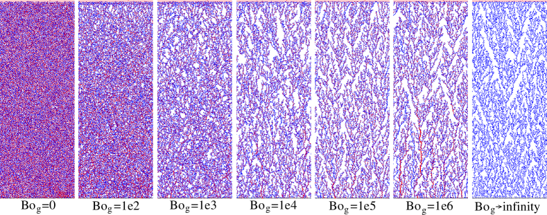
Figure 1: (Color online) Final structures achieved by the deposition/collapse process for different granular Bond numbers $Bo_{g}$. In addition to the particles compressive forces are illustrated by red (dark gray) lines connecting the center of masses between the particles. In the case of $Bo_{g}\to\infty$ no forces are present as it is realized in the simulations by switching off gravity.

In the following, we use monodisperse systems with a friction coefficient $\mu=0.3$ and a rolling friction coefficient of $\mu_{r}=0.1$ (in units of particle radii). The effect of varying these parameters is also studied exemplary and will be discussed later. Typically the values of the density can depend on these parameters as shown in Ref. Bartels et al. (2005) whereas the qualitative behavior does not change. Figure 1 shows the final structures obtained for different values of granular Bond number ranging from $0$ to $10^{6}$. Also the limit of infinite Bond number is shown, leading to pure ballistic deposition Meakin and Jullien (1991) well studied already in the past. For small Bond numbers, here represented by $Bo_{g}=0$, the system typically reaches a random close packing which also has been studied intensively in the past. Note that our case of monodisperse particles typically leads in dense packings to crystallization effects which could be avoided by using a small polydispersity. As our focus in this paper is on the looser structures where this effect is not very important we prefer the monodisperse system to keep the model as simple as possible. In the intermediate range of Bond numbers the density varies between the two limiting values.

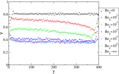
Figure 2: (Color online) Density profiles for different granular Bond numbers $Bo_{g}$ (cf. fig. 1). Here, the volume fraction $\nu$ is plotted. In this case the volume fraction is measured in thin slices of given width (here: $3.97$ particle radii) at varying height $y$. For $Bo_{g}=0$ no cohesion is active and the random close packing is reached. In the limit $Bo_{g}\to\infty$ the system does not collapse at all, and the simple ballistic deposition case Meakin and Jullien (1991) is obtained.

Plotting the density profile depending on the vertical position $y$ (Fig. 2) provides a more quantitative analysis. It can be seen that in the two limiting cases ($Bo_{g}=0$ and $Bo_{g}\to\infty$) the density is constant. For the infinite Bond number this can be explained easily as no collapse at all occurs and the density profile is that of a ballistic deposition and thus constant Meakin et al. (1986); Meakin and Jullien (1991). For the non-cohesive case a close packing is expected, also leading to a constant density. This will be discussed again in more detail later in this paper. In the intermediate range the density decreases with increasing height. This is a result of the generation process where the fragile structure is partially collapsed due to the weight of the added particles which happens discontinuously in relatively small avalanches as will be discussed in more detail in the next section (sec. IV).

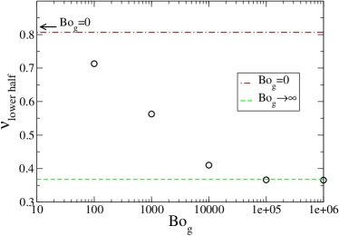
Figure 3: (Color online) Average volume fraction $\nu_{\rm lower\,half}$ depending on granular Bond number $Bo_{g}$. The density is averaged in the lower half of the system excluding the region very close to the bottom to avoid border effects (here we excluded the region below the height of 50 particle radii so that clearly boundary effects are removed for all curves, cf. fig. 2). The volume fractions vary between the two limits given by random close packing ($Bo_{g}=0$) and pure ballistic deposition ($Bo_{g}\to\infty$).

Knowing that the density depends on vertical position a general dependence of the total density on the Bond number cannot easily be defined. Instead, for a given system size as in Fig. 2 the density at a fixed position can be measured. In Fig. 3 the averaged density in the lower half excluding the region very close to the bottom is shown versus the granular Bond number. The density varies between the two limiting cases $Bo_{g}=0$ and $Bo_{g}\to\infty$. Note that the Bond number is plotted in a logarithmic scale, i.e. to see substantial changes of volume fraction the cohesive force or the gravitational force have to be changed by orders of magnitude. Particles with similar gravity and cohesive force will show the same typical behavior. As typically both forces depend on the size of the particles it appears to be natural to characterize the behavior of granular matter and powders by the grain size. For non-cohesive material recent experimental, numerical and theoretical studies Shundyak et al. (2007); Silbert (2010); Farrell et al. (2010); Wang et al. (2010) investigate the influence of the friction coefficient on, e.g. the volume fraction. A similar behavior as found here for the cohesive material when varying the granular bond number, has been found Shundyak et al. (2007); Silbert (2010): varying the friction coefficient on a logarithmic scale leads to a variation between the values $0.84$ for the packing fraction of a random close packing and the value $0.77$ for infinitely large friction coefficient (in two dimensions, in three dimensions between $0.64$ and $0.55$). In the cohesive case as discussed here this range of accessible volume fractions is much higher and limited by the preparation protocol, i.e. in this paper by the ballistic deposition. This limit of course can be changed when changing the preparation protocol, e.g.  by introducing a capture radius (cf. sec. VI).

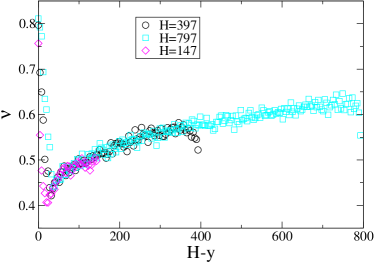
Figure 4: (Color online) Illustration of the effect of system size for intermediate density range (Bond number $Bo_{g}=10^{3}$). Plotting the depth $H-y$ measured from the surface $H$ of the final packings smaller systems show the same profile as large systems.

For all results presented above the total system height $H$ was fixed, i.e. the deposition process stops when no more particles can be deposited below a specified value $H$. When comparing density profiles for different system heights $H$ plots depending on the vertical position $y$ will show different densities. A scaling can be achieved when plotting the density versus the depth $H-y$ as illustrated in Fig. 4. This means the upper part of the large system is depositing and collapsing in the same way as the small system while additionally leading to a further collapse of the structure deposited previously below, accompanied by a downwards motion of the whole upper part. Obviously the slow deposition process guarantees that inertia is not important(cf. sec. VI).

The specific behavior of the density profiles shown in this section results from a deposition process combined with a collapse of the current structure due to gravity. The deposition is characterized by the number of deposited particles per volume, which we call “deposition density” and which here is not constant (sec. V). The collapse happens successively in relatively small avalanches, analyzed in detail in the following section. In section V we will show that these avalanches can be used to relate the final density profile to the “deposition density”.

IV Analysis of the avalanches during deposition/collapsing

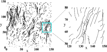
Figure 5: Particle trajectories of particles of the small system ($H=147$, cf. Fig. 4) for the whole deposition/collapse. For better visibility only each 5th particle’s trajectory is shown, i.e. the trajectories of 640 particles (instead of all 3200 particles). Viewing the total system (and on the right more detailed when zooming in) illustrates that parts of the system move collectively downwards accompanied by a sidewards motion or rotation. When zooming in the individual trajectories can be identified which are composed of the sum of paths during all the small avalanches experienced by the particle.

Typically the collapsing of the structures, as mentioned earlier, happens discontinuously in small avalanches. As these avalanches are important also for the final density profiles (see sec. III) their characteristics is studied in detail in this section. To illustrate the nature of these avalanches in Fig. 5 the trajectories of the particles are plotted for a relatively small system of height $H=147$ consisting of about 3200 particles (for better visibility only each 5th trajectory is shown, i.e. the trajectories of 640 particles, instead of all 3200 particles). The avalanches are a collective motion of parts of the system. This mainly downwards motion is accompanied by a sidewards motion or rotation. When zooming in individual trajectories can be identified. These trajectories represent the motion of each particle during deposition/collapsing. Thus, they show the paths that a particle experiences in all avalanches at different times. Neighboring particles can have very similar trajectories, i.e. they belong to the same set of avalanches at different times.

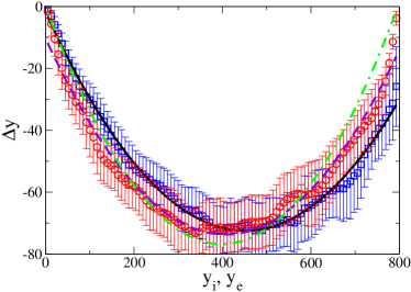
Figure 6: (Color online) Size of avalanches depending on vertical position for $Bo_{g}=10^{3}$. Here the size is measured by $\Delta y$, the average total downwards motion of a particle after deposition (initial position minus final position). On the horizontal axis the initial position $y_{i}$ (blue squares) and final position $y_{e}$ (red circles) are plotted. This leads to two slightly shifted curves as $y_{e}<y_{i}$. The solid lines represent parabolic fits $\Delta y(y_{i})=-1.8-0.31y_{i}+0.00035y_{i}^{2}$ (black, full line) and $\Delta y(y_{e})=-10.2-0.31y_{e}+0.00038y_{e}^{2}$ (violet, dashed). Additionally shown is a fit by $\Delta y(y_{e})=-ay_{e}(1-y_{e}/H)$ predicted by the considerations in sec. VII leading to $a\approx 0.39$ (green, dashed-dotted).

In Figure 6 we show the size of avalanches depending on initial and final vertical position. This size is measured by $\Delta y$, the total downwards displacement of the particle after its deposition, i.e. initial position minus final position. This represents for each particle the sum of all avalanches occurring during the generation process, resulting in as many data points as particles in the system. In Fig. 6 this data is averaged in bins of size two particle diameters. The fluctuations within each bin are shown by the vertical error bars. Both curves (for $y_{i}$ and $y_{e}$) can be relatively well approximated by parabolas:

$$\Delta y(y_{i})=a^{\prime}+b^{\prime}y_{i}+c^{\prime}y_{i}^{2},\quad\Delta y(y_{e})=a+by_{e}+cy_{e}^{2}$$ (1)

It is obvious that both curves cannot obey exactly the parabolic behavior as $y_{i}$ and $y_{e}$ are related by $y_{e}(y_{i})=y_{i}+\Delta y(y_{i})$. However, in the cases presented in this section, obtained by slow deposition, the value of $\Delta y$ is relatively small compared to $y_{i}$ so that $y_{e}(y_{i})$ is very close to a straight line, leading only to a very small horizontal shift. This behavior is typical for intermediate Bond numbers whereas in the limiting cases no noticeable dependence of $\Delta y$ on the vertical position could be found. For $Bo_{g}=0$ a small constant value, below the particle diameter (around $1.5$ particle radii) is observed. In the case $Bo_{g}\to\infty$ no collapse happens, i.e. all $\Delta y=0$.

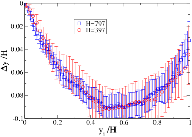
Figure 7: (Color online) Collapse of the size of the avalanches for two different system sizes can be obtained scaling both axes by the system height (here: $Bo_{g}=10^{3}$). Under the assumption of a parabolic profile this scaling leads to a $1/L$ dependence of $c$ (pre-factor of quadratic term in eq. 1).

The parabolic behavior can be reproduced also for other system heights. In Fig. 7 two different system sizes again for $Bo_{g}=10^{3}$ are shown collapsed by scaling both axes by the system height $H$. From this scaling one can deduce the system size dependence of the pre-factor of the quadratic term in eq. (1). The scaling becomes:

$$\Delta y(y,H)=H\cdot f(y/H)\propto H\cdot(y/H)^{2}\propto 1/H$$ (2)

when assuming that $\Delta y\propto y^{2}$ (parabolic behavior, see eq. 1). This $1/H$ dependence could be verified by fitting the curves in Fig. 7. Note that the parabolic shape was also found when varying the friction coefficient $\mu$ and the rolling friction coefficient $\mu_{r}$.

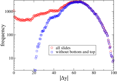
Figure 8: (Color online) The histogram of the size of avalanches $|\Delta y|$ for $Bo_{g}=10^{3}$ follows basically a Gaussian. Deviation from this behavior can almost fully be suppressed when removing the bottom and top part of the system.

Whereas the average of the avalanche size $\Delta y$ as function of the vertical position shows a parabolic profile of reasonable quality, there are of course large fluctuations around this value. In Fig. 8 we show the distribution of the avalanche sizes (here $|\Delta y|$) for the entire system, i.e. independent on the vertical position. When removing the upper and lower part of the system to decrease boundary effects we obtain a Gaussian distribution, i.e. we get an estimate of a typical avalanche size. This typical size decreases with increasing Bond number, and in the limit of $Bo_{g}\to\infty$, where no avalanches occur, it vanishes.

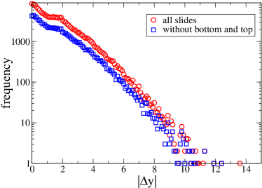
Figure 9: (Color online) The histogram of avalanches $|\Delta y|$ for $Bo_{g}=0$ basically shows an exponential decay. Deviation from this behavior can be found for $|\Delta y|$ between 1 and 2 particle radii where the probability is about constant. This effect cannot be suppressed when removing the bottom and top part of the system (as, e.g.  for $Bo_{g}=10^{3}$).

In the limit of $Bo_{g}=0$ (no cohesion) the behavior is different, an exponential decay is obtained (Fig. 9). Here the boundaries have no effect, i.e. we get the same behavior when removing the upper and lower part of the system as done previously. For this Bond number typically the surface of the structure during deposition grows relatively flat, so that large $|\Delta y|$ are unlikely as expressed by the exponential decay. Due to the monodispersity this surface is locally almost a flat crystalline surface with heaps which consists of a few particles only, in most cases one particle. When a particle is deposited on a one particle heap it rolls off to rest eventually as a “crystalline” neighbor aside the particle, resulting in $|\Delta y|$ between one and two. This leads to the very small range of $|\Delta y|$ with constant probability in Fig. 9. Taking a slightly polydisperse system this region would disappear.

In this section we studied the collapse of the structures occurring in small avalanches we analyzed statistically. We suggest to characterize these avalanches by their “size”, showing a typical dependence on vertical position, a parabolic shape for the specific systems investigated in this section. In the following section we will use this characteristic behavior to be able to derive the final density profile from the “deposition density”. In section VI the same concept will be shown to be applicable also for other protocols of generating loose structures.

V Theoretical analysis of the avalanches

In the previous sections we mentioned that the dynamics leading to a final configuration is determined by small avalanches occurring during the deposition process. All these compaction events contained in the function $\Delta y(y_{e})$, which is given by the difference between the initial position $y_{i}$ and final position $y_{e}$. Note that $\Delta y$ can be plotted (e.g. fig. 6) as function of the final position $y_{e}$ or alternatively as function of the position of deposition $y_{i}$. The aim of this section is to relate the final density profile to the dynamic process of deposition and collapse by using $\Delta y(y_{e})$, showing how the avalanches produce the final density $\rho_{f}(y_{e})$ from the deposition density $\rho_{d}(y_{i})$. The deposition density is defined by the number of particles deposited within a volume. As the structure collapses between the depositions the deposition density is not independent on the collapsing, and it is possible that at (almost) the same position several particles are deposited. Thus, locally within a fixed volume even more particles could be deposited than typical for a dense packing.

We first calculate the number $N_{d,f}$ of particles up to a given height $y_{i,e}$ ($L_{x}$ width of the two dimensional system in units of particle radii):

$$N_{d,f}(y_{i,e})=L_{x}\int_{0}^{y_{i,e}}dy^{\prime}\rho_{d,f}(y^{\prime})$$ (3)

The final position $y_{e}$ of particles can be related to the position $y_{i}$ of deposition by the avalanche profile $\Delta y$:

$$y_{i}(y_{e})=y_{e}-\Delta y(y_{e}),\qquad\mbox{or }\quad y_{e}(y_{i})=y_{i}+\Delta y(y_{i})$$ (4)

In this notation $\Delta y$ is negative as the motion of the particles is downwards (due to gravity). Therefore, $y_{i}$ is larger than or equal to $y_{e}$. As particles are never destroyed the number of particles deposited up to a given height, $N_{d}(y_{i})$, will stay the same, but shifted to a lower height, $N_{f}(y_{e})$, where $y_{i}$ and $y_{e}$ are related by eq. (4). Together with eq. (3) this leads to:

$$N_{f}(y_{e})/L_{x}=N_{d}(y_{i}(y_{e}))/L_{x}=\underbrace{\int_{0}^{y_{i}(y_{e})}dy^{\prime}\rho_{d}(y^{\prime})}_{\equiv G(y_{i}(y_{e}))}$$ (5)

This relates $N_{f}$ to the deposition density whereas eq. (3) relates $N_{f}$ to the final density. The function $G$ here is formally introduced for the integral as abbreviation, by derivation of $G$ the density is retrieved. The final density can be obtained by derivation of $N_{f}/L_{x}$ using eq. (5):

$$\rho_{f}(y_{e})=\frac{d}{dy_{e}}\frac{N_{f}(y_{e})}{L_{x}} = \frac{d}{dy_{e}}G(y_{i}(y_{e}))=\frac{dG(y_{i})}{dy_{i}}\frac{dy_{i}}{dy_{e}}$$

$$= \rho_{d}(y_{i}(y_{e}))\frac{dy_{i}}{dy_{e}}$$

$$= \rho_{d}(y_{i}(y_{e}))\left(1-\frac{d\Delta y(y_{e})}{dy_{e}}\right)$$

The deposition density $\rho_{d}(y_{i}(y_{e}))$ in principle can be expressed directly by $y_{e}$ introducing $\rho_{d}^{\prime}(y_{e})$. As usually the functional behavior of both functions is not known, but only values for specific $y_{i}$ and $y_{e}$, the transformation can be done for each point by simply using eq. (4), i.e. replacing each $y_{i}$ by $y_{e}=y_{i}+\Delta y(y_{i})$. Summarizing, to calculate the final density profile one needs to know the deposition density $\rho_{d}$ and the avalanche profile $\Delta y$. Note that the avalanche profile dependence on both $y_{e}$ and $y_{i}$ is needed, which can be calculated from each other for some cases as shown later. For experimental situations these quantities are not known. However, the relation between $\rho_{f}$ and $\rho_{d}$ (eq. V) can be used to calculate the deposition density from the final density in the slow deposition limit, when assuming a parabolic profile as found in the simulations before.

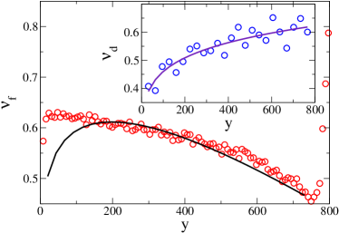
Figure 10: (Color online) Using the parabolic approximation (fig. 6) for the average avalanches the final density (here volume fraction $\nu_{f}$) can be calculated from the deposition density (here shown: volume fraction $\nu_{d}$ for $Bo_{g}=10^{3}$, inset). There are strong fluctuations in the deposition density which are induced by the irregularity of the avalanches. To obtain a smooth curve we use a fit function (here: power law fit, with exponent $0.15$) to calculate the final density (black line) matching relatively well with the measured density profile for sufficiently large $y$ (except close to the bottom)

In figure 10 we use eq. (V) to calculate the final density from the deposition density by using the parabolic fit for $\Delta y$ (fig. 6). In practice first the deposition density curve is shifted on the horizontal axis by $y_{e}=y_{i}-(a^{\prime}+b^{\prime}y_{i}+c^{\prime}y_{i}^{2})$, then multiplying the deposition density with the right hand side of eq. (V), $1-(b+2cy_{e})$, i.e. using the derivative of $\Delta y(y_{e})$ which is a linear function. If the deposition density would be constant this would lead to a linear profile for the final density. However, the deposition density is not constant, explaining the non-linear behavior for the final density. Additionally the deposition density shows strong fluctuations, but by assuming the avalanches to follow the averaged parabolic behavior the corresponding fluctuations in the avalanche profile are not included. The calculated curve matches relatively well the profile measured in the simulations for sufficiently large values of the vertical position. Close to the bottom, however, the calculated curve deviates from the measured one. In this region the deposition density is very small, i.e. almost the one of pure ballistic deposition. This can be understood as the system needs to gain a sufficient amount of weight for the collapse to start (cf. also sec. VI). This should correspond to a higher initial slope of $\Delta y(y_{e})$ which is not reflected in the parabolic approximation (eq. 1). In this region a higher order terms would be necessary for reproducing also the system bottom.

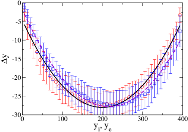
Figure 11: (Color online) Size of avalanches depending on vertical position for $Bo_{g}=10^{2}$. Here the size is measured by $\Delta y$, the total downwards motion of the particle after deposition (initial position minus final position). On the horizontal axis the initial position $y_{i}$ (blue squares) and final position $y_{e}$ (red circles) are plotted. The lines represent the parabolic fits $\Delta y(y_{i})=-1.7-0.24y_{i}+0.00056y_{i}^{2}$ (dashed, violet) and $\Delta y(y_{e})=-4.7-0.23y_{e}+0.00059y_{e}^{2}$ (full line, black).

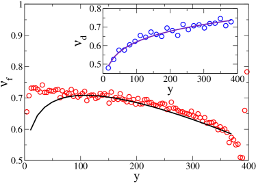
Figure 12: (Color online) Using the parabolic approximation (fig. 11) for the average avalanches the final density can be calculated from the deposition density (here shown: volume fraction for $Bo_{g}=10^{2}$). There are strong fluctuations in the deposition density which are induced by the irregularity of the avalanches. As before (for $Bo_{g}=10^{3}$), to obtain a smooth curve we use a fit function (here: power law fit, with exponent 0.13) to calculate the final density (black line) matching relatively well for sufficiently large $y$ (except close to the bottom).

The same analysis has been done also, e.g. for $Bo_{g}=10^{2}$ as shown in Figs. 11 and 12. In this case the deposition density shows somewhat lower fluctuations as for $Bo_{g}=10^{3}$ (Fig. 10). To quantify this we estimated the fluctuations of the deposition density at vertical position $y=200$ for both cases. For $Bo_{g}=10^{2}$ we obtained around 15% whereas we estimated around 20% for $Bo_{g}=10^{3}$. For the case of $Bo_{g}\to\infty$ there is no avalanching at all (cf. sec. IV), and trivially the final density equals the deposition density. This is very similar for very large $Bo_{g}$, but as some avalanches occur there are some relatively small fluctuations in the average profile. Away from this limit, but still close enough that the density profile is very similar to the $Bo_{g}\to\infty$ case, as e.g.  for $Bo_{g}=10^{4}$, very large fluctuations in the avalanche profile are observed. Thus, the parabolic profile cannot easily be identified. Still the theory works well as the final density is very close to the deposition density so that even a very inaccurate fit for the avalanche profile does not affect the calculated density profile too much. In the limit of $Bo_{g}=0$ the avalanche profile is a constant (cf. sec. IV), i.e.  all grains are slightly shifted downwards by the same amount (except boundary effect at the bottom). As then the derivative vanishes the final density equals the deposition density.

Here, we showed how the parabolic avalanche profile can be used to calculate the final density profiles from the deposition density in the case where gravity acts during deposition. In the next section the same concept will be used to the simpler case of collapse of the system after deposition is complete. These two cases could be then related in section VII.

VI Collapse after deposition complete

In the previous sections we investigated the case where gravity acts during deposition, leading to relatively complex shape of the density profiles and a parabolic characteristics of the avalanche size. For this case we showed that these avalanche profiles can be used to relate the final density profile to the deposition density. In this section we will analyze the case when the particles are first deposited, then gravity is switched on and the structures collapse. This case is even simpler and can later be used to understand the more complex system studied before. In this case the initial density $\rho_{i}$ characterizes the system (instead of the deposition density as in the previously discussed situation).

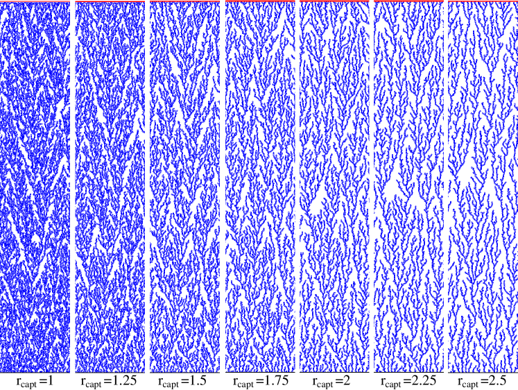
Figure 13: Initial structures generated by ballistic deposition with increasing capture radius $r_{\rm capt}$.

Using the off lattice version of ballistic deposition as presented in Refs. Meakin et al. (1986); Meakin and Jullien (1991) with sticking probability one, vertically falling particles stick when they touch an already deposited particle. This leads to a fixed initial density. Lower densities can be obtained by using a capture radius $r_{\rm capt}$ i.e. particles stick to each other when they are within a certain distance during the falling of the depositing particle. More precisely: When the distance between the center of masses of two particles is below $2\cdot r_{\rm capt}$ the particles stick and the falling particle is pulled along the connecting line towards the already deposited particle. This capture radius is a measure for the distance between the branches of the deposit and the resulting density is inversely proportional to $r_{\rm capt}$ Kadau et al. (2003a), $r_{\rm capt}=1$ gives the original method. The resulting initial structures are shown in Fig. 13. These structures obtained with different capture radius will be later used to study the influence of the initial density.

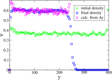
Figure 14: (Color online) The initial and final density are about constant when depositing first and then collapsing the system ($Bo_{g}=10^{3}$). Using the linear dependence of the avalanches $\Delta y$ on the vertical position (see Fig. 15) the final density can be calculated from the initial density using eqs. (4) and (V). The results support the analytical considerations.

First we will investigate the behavior using $r_{\rm capt}=1$. Figure 14 shows the density profile before the collapse which is the same that we got in the limit of $Bo_{g}\to\infty$ in sec. III, also independent on vertical position. After this deposition is complete gravity is “switched on” and the structure abruptly collapses. Here we choose a Bond number of $Bo_{g}=10^{3}$. This leads to a final structure with higher density, in this case also independent on the vertical position (Fig. 14). As no particles are added after the initial deposition the final system height is lower.

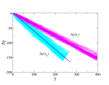
Figure 15: (Color online) The linear dependence of the avalanche sizes $\Delta y(y_{i,e})$ explains the homogeneous density increase as seen in fig. 14. The linear fits are $\Delta y(y_{e})=2.2-0.62y_{e}$ and $\Delta y(y_{i})=1.9-0.39y_{i}$.

Similarly as we did before we analyze the size of the avalanches $\Delta y$ as defined in sec. IV. Figure 15 shows a linear dependence of $\Delta y$ on either $y_{e}$ and $y_{i}$. The fit parameters of the two lines can be related to each other by the relation between $y_{i}$ and $y_{e}$ (eq. 4). Assuming $\Delta y(y_{e})=a-by_{e}$ and $\Delta y(y_{i})=a^{\prime}-b^{\prime}y_{i}$ the values $a^{\prime}$ and $b^{\prime}$ can be calculated from $a$ and $b$ (see app. A) as:

$$b^{\prime}=\frac{b}{1+b},\quad a^{\prime}=\frac{a}{1+b}$$ (7)

The vertical dependence of $\Delta y$ can be used similarly as before to calculate the final density from the initial density by using eq. (V). The calculated density profile using this linear dependence reproduces the obtained final density profile very well as shown in Fig. 14. In this case the agreement is better as now the initial density is not fluctuating very much in contrast to the cases discussed in sec. V. The density increase $\Delta\rho$ (or volume fraction increase $\Delta\nu$) can be directly calculated by the constant slope of $\Delta y(y_{e})$:

$$\frac{\Delta\rho}{\rho_{i}}=\frac{\Delta\nu}{\nu_{i}}=-\frac{d\Delta y(y_{e})}{dy_{e}}$$ (8)

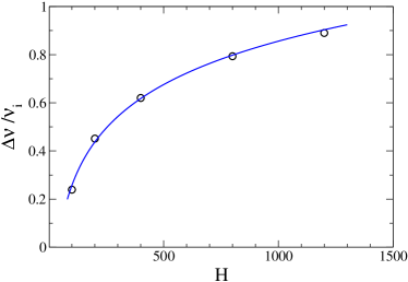
Figure 16: Dependence of volume fraction increase $\Delta\nu/\nu_{i}$ on system height $H$ when first deposited and then collapsed. A logarithmic fit matches the data best (here $y=-0.94+0.26\ln(x)$). The limit of random close packing defines the largest possible value for $\Delta\nu/\nu_{i}$ of $1.19$, which will be approached for infinite system heights.

For the same parameters ($Bo_{g}=10^{3}$) we studied the effect of the system height $H$ on the density increase while still keeping the initial density fixed (fig. 16). A logarithmic fit matches the data best. This fit certainly cannot continue to infinity as there is a limit for the density $\rho_{\rm max}$ given by the random close packing (see also fig. 3), leading to a $(\Delta\nu/\nu_{i})_{\rm max}$ of $1.19(\simeq\rho_{\rm max}/\rho_{\rm ini}-1)$.

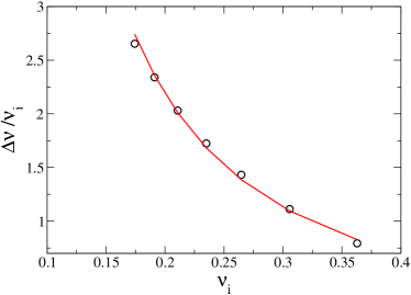
Figure 17: Dependence of volume fraction increase $\Delta\nu/\nu_{i}$ on volume fraction $\nu_{i}$ of the initial system (system first deposited and then collapsed). Different densities could be reached by increasing the capture radius for ballistic deposition (fig. 13). A power law fit with exponent $1.64$ fits relatively well (power law fit results in $y=0.158x^{-1.64}$).

Using initial capture radii as described above we study the influence of the initial density on the relative density increase $\Delta\nu/\nu_{i}$ (fig. 17). We could obtain the best fit when using a power law with exponent of about $1.64$.

We showed in this section that the linear avalanche profile is a characteristic feature of compacting from a depth independent to a depth independent structure, obtained here for systems generated by ballistic deposition collapsing due to gravity. More complex avalanche profiles with non-constant derivative will transform homogeneous structures into inhomogeneous structures. Thus, we expect the linear profile to be obtained in all cases where a homogeneous initial system compacts to a homogeneous final system. These homogeneous compaction processes are investigated in different research areas as e.g. discussed in Refs. Kjeldsen et al. (2006); Lumay and Vandewalle (2007); Dong et al. (2006); Valverde and Castellanos (2006); Son et al. (2008). In addition in the next section we will show that also for the more complex process when gravity acts during deposition (sec. III) this linear profile can be used to derive the parabolic profile of the avalanches.

VII Relation between deposition under gravity and switching on gravity after deposition

For the very fast process a linear profile for $\Delta y$ depending on vertical position has been found (cf. fig. 15) whereas the slow deposition limit shows a parabolic profile for $\Delta y$ depending on vertical position (cf. figs. 6,11). In this section we will discuss how a relation between both can be established. By this relation also the parabolic profile is put onto a more fundamental basis like the linear profile for the homogeneous collapse.

Let us imagine depositing particles slice by slice as sketched in Fig. 18.

Figure 18: Sketch illustrating the procedure of depositing the grains slice by slice. The first slice deposited is compacted by internal collapse. The same is true for each “freshly” deposited slice. The slices below are compacted by the added weight of the slices above. Periodic boundary conditions in horizontal direction are imposed (illustrated by dashed lines). The figure also illustrates the definition of the symbols used here. The $n$ slices are numbered from $1$ to $n$. A slice $i$ collapses from $\rho_{i-1}$ to $\rho_{i}$ while its height decreases from $h_{i-1}$ to $h_{i}$, where $h_{i}=\rho_{i-1}/\rho_{i}h_{i-1}$.

The slices are thin parts of the system in vertical direction spanning the full system width in horizontal direction. They can be considered as systems with very small initial height $h_{0}$. In each slice the deposition will be immediately followed by the collapse. However, there will be not only an “internal collapse” within the “freshly” deposited slice, but also a compaction of the slices below due to the additional weight of the “freshly” deposited slice.

Let us first consider systems composed of a small number $n$ of slices. The case $n=1$ (one slice) is the same as discussed in the previous section: The system collapses “internally” leading to an increase of the density from $\rho_{0}$ to $\rho_{1}$ while the height reduces from $h_{0}$ to $h_{1}$. Here we denote the slice number as $1$ (cf. Fig. 18). As shown in the previous section the avalanche sizes have a linear profile $\Delta y(y_{e}^{(1)})=S_{1}y_{e}^{(1)}$. $S_{1}$ is the slope in slice $1$, and is the same for all freshly deposited slices when the height $h_{0}$ is kept constant. The vertical position $y_{e}^{(1)}$ within slice $1$ is measured from its bottom ($y_{e}^{(1)}=0\dots h_{1}$). This notation will be used in the following for each slice $i$: $y_{e}^{(i)}=0\dots h_{i}$. The case $n=2$ (two slices) means adding an additional slice to the case $n=1$. Then the lower slice (slice 2) experiences an additional compaction by the added weight expressed by the corresponding avalanche size $C_{2}y_{e}^{(2)}$ assuming a linear behavior for this relatively fast process similar as for the internal collapse. This is justified at least for the limit of small slices later considered in this section. The upper slice (slice 1) will be compacted internally and additionally will move downwards by $C_{2}h_{2}$ ($=h_{1}-h_{2}$) as the slice below is compacted. Summarizing for the two slices we get:

$$\Delta y^{(1)}(y_{e}^{(1)}) = S_{1}y_{e}^{(1)}+\underbrace{C_{2}h_{2}}_{h_{1}-h_{2}}$$ (9)

$$\Delta y^{(2)}(y_{e}^{(2)}) = C_{2}y_{e}^{(2)}+S_{1}\underbrace{(1+C_{2})y_{e}^{(2)}}_{y_{e}^{(1)}}$$

For slice 2 the internal compaction from the first step $S_{1}y_{e}^{(1)}$ has been transformed by using that $\rho_{2}=(1+C_{2})\rho_{1}$ (cf. eq. 8), leading to $h_{2}=\rho_{1}/\rho_{2}h_{1}=1/(1+C_{2})h_{1}$. Adding a further slice leads to the case $n=3$, where the two slices are compacted due to the additional weight. Each of these compactions is accompanied by a downwards shift of the slices above. This leads to:

$$\Delta y^{(1)}(y_{e}^{(1)}) = S_{1}y_{e}^{(1)}+\underbrace{C_{2}h_{2}+C_{3}h_{3}}_{(h_{1}-h_{2})+(h_{2}-h_{3})=h_{1}-h_{3}}$$ (10)

$$\Delta y^{(2)}(y_{e}^{(2)}) = C_{2}y_{e}^{(2)}+\underbrace{S_{1}(1+C_{2})y_{e}^{(2)}+C_{2}h_{2}}_{\mbox{from step 2}}+C_{3}h_{3}$$

$$\Delta y^{(3)}(y_{e}^{(3)}) = C_{3}y_{e}^{(3)}$$

$$+\underbrace{C_{2}(1+C_{3})y_{e}^{(3)}+S_{1}(1+C_{2})(1+C_{3})y_{e}^{(3)}}_{\mbox{from step 2}}$$

Imagining continuing this iterative procedure, one obtains the case of $n$ slices. For the top slice this results in:

$$\Delta y^{(1)}(y_{e}^{(1)}) = S_{1}y_{e}^{(1)}+\underbrace{C_{2}h_{2}+C_{3}h_{3}+\dots+C_{n}h_{n}}_{h_{1}-h_{n}}$$ (11)

The first term is the internal collapse where the other terms are the shift due to the compaction of all slices below ($2$ to $n$) in this last step. For the bottom slice we get:

$$\Delta y^{(n)}(y_{e}^{(n)}) = S_{1}(1+C_{2})(1+C_{3})\cdot\ldots\cdot(1+C_{n})y_{e}^{(n)}$$

$$C_{n}y_{e}^{(n)}+C_{n-1}(1+C_{n})y_{e}^{(n)}+\dots$$

$$+C_{2}(1+C_{n})(1+C_{n-1})\cdot\ldots\cdot(1+C_{3})y_{e}^{(n)}$$

Here all terms represent a collapse in the slice either internally by its own weight when deposited in the first step, or when collapsing due to added weight in the following steps. In addition these collapses have to be transformed to a $y_{e}^{(n)}$ dependence (see above). For an arbitrary slice $i$ somewhere in the system we get both types of terms as in eqs. (11) and (VII):

$$\Delta y^{(i)}(y_{e}^{(i)}) = S_{1}(1+C_{2})\cdot\ldots\cdot(1+C_{i})y_{e}^{(i)}$$

$$C_{i}y_{e}^{(i)}+C_{i-1}(1+C_{i})y_{e}^{(i)}$$

$$+\dots+C_{2}(1+C_{3})\cdot\ldots\cdot(1+C_{i})y_{e}^{(i)}$$

$$\underbrace{+C_{n}h_{n}+C_{n-1}h_{n-1}+\dots+C_{n-i+1}h_{n-i+1}}_{h_{n-i}-h_{n}}$$

$$\underbrace{+C_{n-1}h_{n-1}+\dots+C_{n-i}h_{n-i}}_{h_{n-i-1}-h_{n}}$$

$$\vdots$$

$$\underbrace{+C_{i+1}h_{i+1}+\dots+C_{2}h_{2}}_{h_{1}-h_{i+1}}$$

The part of the expression independent on $y_{e}^{(i)}$ represents the shift due to compaction by the weight of the above added slices in $n-i$ steps considering all slices below. It consists of $n-i$ times $i-1$ terms and can be written shortly as:

$$\Delta y^{(i)}_{\rm shift} = \sum_{j=1}^{n-i}h_{j}-h_{j+i}$$ (14)

The limit of large $n$ while keeping the total system height constant gives very small slices where the part $\Delta y^{(i)}_{\rm shift}$ dominates as for very small systems the internal collapse almost vanishes (cf. fig. 16). Therefore, in the following we will only consider this term to show that we approximately obtain a parabolic behavior. Let us assume that the $h_{i}$ are linear in $i$:

$$h_{i}=\left(1-a\frac{i}{n}\right)h_{0},\qquad a<1$$ (15)

This means that deeper in the system (larger $i$) the width of the slice is smaller. Note that for the case $a\ll 1$ this can be understood as a linearization. This case means that the overall compaction is not large as it is the case for intermediate Bond numbers. From eqs. (15) and (14) we obtain:

$$\Delta y^{(i)}_{\rm shift} = \sum_{j=1}^{n-i}\left(1-a\frac{j}{n}\right)h_{0}-\left(1-a\frac{j+i}{n}\right)h_{0}$$ (16)

$$= \sum_{j=1}^{n-i}a\frac{i}{n}h_{0}=(n-i)a\frac{i}{n}h_{0}$$

This is a quadratic dependence on the slice number $i$. To compare to our results we have to transform $i$ to vertical position $y_{e}$, which is obtained when summing up the height $h_{i}$ of all slices:

$$y_{e}(i)=\sum_{j=n}^{i+1}h_{j}=\sum_{j=1}^{n-i}h_{j+i}$$ (17)

Using the approximation (15) we obtain:

$$y_{e}(i) \simeq \sum_{j=1}^{n-i}\left(1-a\frac{j+i}{n}\right)h_{0}$$ (18)

$$= h_{0}\left[n-\frac{a}{2}(n^{2}-n)\right]-ih_{0}\left[1-a(n-1/2)\right]$$ (19)

The detailed derivation is given in appendix B. From this equation we can obtain $i(y_{e})$:

$$i=\frac{-y_{e}}{h_{0}\left[1-a(n-1/2)\right]}+\frac{n-a/2(n^{2}-n)}{1-a(n-1/2)}$$ (20)

We assume that we are in the limit of relatively small $a$. Neglecting all terms in $a$ in eq. (20) corresponds to neglecting terms in $a^{2}$ in eq. (16). With this simplification additionally using $h_{0}=H/n$ we obtain $i=n-y_{e}/h_{0}=n(1-y_{e}/H)$, leading to:

$$\Delta y_{\rm shift}(y_{e}(i)) = [n-i(y_{e})]i(y_{e})\frac{Ha}{n^{2}}$$ (21)

$$= ay_{e}\left(1-\frac{y_{e}}{H}\right)$$ (22)

This behavior is plotted in fig. 6 (green curve). Note that in this figure the $\Delta y$ is negatively defined as opposed to the definition used in this section. This curve fits relatively well the measured curves except coming close to the top. This can be explained by the existence of a small “crust”, i.e. an accumulation of particles at the top of the system in the simulations which is not considered in the analysis in this section. Probably this is also the reason for the slightly different pre-factors of the parabola: From eq. (22) we obtain $a=0.39$ leading to a pre-factor of the quadratic term of $a/H=0.00049$ which is somewhat larger than the value obtained previously of $0.00038$. The value of $a=0.39$ is at least reasonably small to ensure that the considerations of this section agree roughly with the simulation results. Previously by scaling $\Delta y$ for different system sizes we obtained that the pre-factor of the parabola scales as $1/H$ (cf. eq. 2). This implies that $a$ is independent on system size $H$, for each specific Bond number, additionally indicating by its value how good the approximations of this section are.

Thus, in the limit of small $a$ we could show that the linear behavior of $\Delta y$ when collapsing after deposition complete leads to a parabolic behavior when collapsing during deposition. Note that this $a$ represents the differences in heights of the top and the bottom slice, i.e. the assumption of small $a$ is true when the density difference between the density close to the bottom and at the top is small which is the case in all our cases studied here (cf. Fig. 2). In the structures studied within our model in the previous sections (see e.g. sec. III) a small “crust” (particle accumulation) at the top leads to a density increase again. This will lead to a shift in the parabolic profile to the right (to the top). As we discussed previously the deposition/collapse process is not continuous, so that the parabola is only an average of a very noisy distribution of $\Delta y$. Additionally, the deposition density is not constant, but slightly increasing (cf. figs. 10 and 12) accompanied by relatively large fluctuations. For these reasons we can only expect a rough matching of our theory with the simulations. Nevertheless the parabolic behavior has been observed relatively clearly.

VIII Conclusion/Outlook

We studied the generation of fragile granular structures by a deposition/collapse process. In one extreme case where the deposition is sufficiently slow to allow the system to collapse and relax due to gravity after the deposition of each single grain we studied the influence of the granular Bond number on the density profile. For intermediate Bond numbers the density decreases with height due to the compaction of the powder’s own weight. We studied the generation process dynamics which is discontinuous in small avalanches. These avalanches showed a parabolic behavior and can be used to calculate the final density profile from the deposition density. In the other extreme case of collapse after deposition complete we found that the density is constant with vertical position, and that the avalanche size depends linearly on vertical position. We could relate the parabolic behavior to the linear one by imagining a slice by slice deposition/collapse process. Note that the linear behavior investigated here for the case of ballistic deposition followed by a gravitational collapse will be found for all collapse/compaction processes of homogeneous initial structures to homogeneous final structures. Therefore the concept of avalanches introduced in this paper is of general applicability to granular structures collapsing due to gravity or similar forces.

Our results maybe directly verified experimentally, as already mentioned in the introduction, e.g. by using a Hele Shaw cell Völtz et al. (2000, 2001); Vinningland et al. (2007) which can be tilted to effectively change gravity. To apply the model presented here more specifically, e.g. for snow compaction, more realistic microscopic properties including aging processes would have to be used. For cake formation processes, instead of gravity a porosity dependent drag force could be applied. In this context an explicit consideration of the pore fluid/gas could be needed. The influence of the pore fluid/gas should be in particular studied for the fast compaction process presented in this paper.

Appendix A Relation between slopes

The linear dependence of avalanches is found as well in $y_{e}$ as in $y_{i}$ (see fig. 15). In this section the relation between the two lines is derived in detail. Assuming

$$\Delta y(y_{e})=a-by_{e}\mbox{ and }\Delta y(y_{i})=a^{\prime}-b^{\prime}y_{i}$$ (23)

the values $a^{\prime}$ and $b^{\prime}$ can be calculated from $a$ and $b$ as shown in the following. The relation between $y_{i}$ and $y_{e}$ can be written as:

$$y_{i}=y_{e}-\Delta y(y_{e}) = y_{e}-(a-by_{e})$$ (24)

$$= y_{e}(1+b)-a$$ (25)

$$\Longrightarrow y_{e} = \frac{a}{1+b}+\frac{\overbrace{1}^{1+b-b}}{1+b}y_{i}$$ (26)

$$= y_{i}\left(1-\frac{b}{1+b}\right)+\frac{a}{1+b}$$ (27)

According to (4) and (23) $y_{e}$ can be written as:

$$y_{e}=y_{i}+(a^{\prime}-b^{\prime}y_{i})$$ (28)

Comparing (27) and (28) results in:

$$b^{\prime}=\frac{b}{1+b},\quad a^{\prime}=\frac{a}{1+b}$$ (29)

From this or by a similar derivation the inverse relations can also be obtained:

$$b=\frac{b^{\prime}}{1-b^{\prime}},\quad a=\frac{a^{\prime}}{1-b^{\prime}}$$ (30)

Appendix B Derivation of $y_{e}(i)$ in linear approximation for $h_{i}$

Here we show the details of the derivation to obtain eq. (19) from eq. (18):

$$y_{e}(i)\simeq\sum_{j=1}^{n-i}\left(1-a\frac{j+i}{n}\right)h_{0}$$

$$= h_{0}(n-i)-\frac{ha}{n}\left(\underbrace{\sum_{j=1}^{n-i}i}_{(n-i)i}+\underbrace{\sum_{j=1}^{n-i}j}_{(n-i+1)(n-i)/2}\right)$$

$$= h_{0}(n-i)-h_{0}a(n-i)i/n-h_{0}a(n-i+1)(n-i)/2$$

$$= h_{0}(n-i)-h_{0}a\left[\frac{n}{2}(n+1)-i\left((n+1)/2+n/2\right)\right]$$

$$= h_{0}\left[n-\frac{a}{2}(n^{2}-n)\right]-ih_{0}\left[1-a(n-1/2)\right]$$

References

- Mitchell and Soga (2005) J. Mitchell and K. Soga, Fundamentals of soil behavior (Wiley, Hoboken, New Jersey, 2005), 3rd ed.
- Barden et al. (1973) L. Barden, A. McGown, and K. Collins, Engineering Geology 7, 49 (1973).
- Assallay et al. (1997) A. Assallay, C. Rogers, and I. Smalley, Engineering Geology 48, 101 (1997).
- Reznik (2005) Y. Reznik, Eng. Geol. 78, 95 (2005).
- Rognon et al. (2006a) P. G. Rognon, J.-N. Roux, D. Wolf, M. Naa m, and F. Chevoir, EPL (Europhysics Letters) 74, 644 (2006a).
- Wagner and Brady (2009) N. J. Wagner and J. F. Brady, Physics Today 62, 27 (2009).
- Gado and Kob (2010) E. D. Gado and W. Kob, Soft Matter 6, 1547 (2010).
- Kadau et al. (2009a) D. Kadau, H. Herrmann, J. Andrade Jr., A. Araújo, L. Bezerra, and L. Maia, Brief Communications to Granular Matter 11, 67 (2009a).
- Kadau et al. (2009b) D. Kadau, H. Herrmann, and J. Andrade Jr., Eur. Phys. J. E 30, 275 (2009b).
- Manley et al. (2005) S. Manley, J. Skotheim, L. Mahadevan, and D. Weitz, Phys. Rev. Lett. 94, 218302 (2005).
- Wu et al. (2005) Q. Wu, Y. Andreopoulos, S. Xanthos, and S. Weinbaum, J. Fluid Mech. 542, 281 (2005).
- Heierli (2005) J. Heierli, J. Geophys. Res. [Earth Surface] 110, F02008 (2005).
- Kadau et al. (2009c) D. Kadau, H. Herrmann, and J. Andrade Jr., in Powders and Grains 2009, edited by M. Nakagawa and S. Luding (Amer. Inst. Physics, 2009c), vol. 1145 of AIP Conference Proceedings, pp. 981–984.
- Bürger et al. (2001) R. Bürger, F. Concha, and K. H. Karlsen, Chem. Eng. Sci. 56, 4537 (2001).
- Aguiar and Coury (1996) M. L. Aguiar and J. R. Coury, Ind. Eng. Chem. Res. 35, 3673 (1996).
- Stamatakis and Tien (1991) K. Stamatakis and C. Tien, Chem. Eng. Sci. 46, 1917 (1991).
- Lu and Hwang (1995) W.-M. Lu and K.-J. Hwang, AIChE 41, 1443 (1995).
- Ling (1985) C.-H. Ling, J. of Glaciology 31, 194 (1985).
- Kaempfer and Schneebeli (2007) T. U. Kaempfer and M. Schneebeli, J. Geophys. Res. 112 (2007).
- Vetter et al. (2010) R. Vetter, S. Sigg, H. Singer, D. Kadau, H. Herrmann, and M. Schneebeli, Eur.Phys.Lett. 89, 26001 (2010).
- Bahr et al. (2001) D. B. Bahr, E. W. H. Hutton, J. P. M. Syvitsky, and L. F. Pratson, Computers & Geosciences 27, 691 (2001).
- Bayer (2989) U. Bayer, Geologische Rundschau 78, 155 (2989).
- Athy (1930) L. F. Athy, Bull. Amer. Assoc. Petrol. Geol. 14, 1 (1930).
- Roeck et al. (2008a) M. Roeck, M. Morgeneyer, J. Schwedes, L. Brendel, D. Wolf, and D. Kadau, Particulate Science and Technology 26, 43 54 (2008a).
- Roeck et al. (2008b) M. Roeck, M. Morgeneyer, J. Schwedes, D. Kadau, L. Brendel, and D. Wolf, Granular Matter 10, 285 293 (2008b).
- Araújo et al. (2006) A. D. Araújo, J. S. A. Jr., and H. J. Herrmann, Phys. Rev. Lett. 97, 138001 (2006).
- Kennedy et al. (2003) M. K. Kennedy, F. E. Kruis, H. Fissan, B. R. Mehta, S. Stappert, and G. Dumpich, J. Appl. Phys. 93, 551 (2003).
- Moreau (1994) J. J. Moreau, Eur. J. Mech. A-Solid 13, 93 (1994).
- Jean and Moreau (1992) M. Jean and J. J. Moreau, in Contact Mechanics International Symposium (Presses Polytechniques et Universitaires Romandes, Lausanne, 1992), pp. 31–48.
- Unger and Kertesz (2003) T. Unger and J. Kertesz, in Modelling of Complex Systems (American Inst. of Physics, Melville, New York, 2003), pp. 116–138.
- Brendel et al. (2004) L. Brendel, T. Unger, and D. Wolf, in The Physics of Granular Media, edited by H. Hinrichsen and D. Wolf (Wiley-VCH, Weinheim, 2004), pp. 325–340.
- Kadau et al. (2003a) D. Kadau, G. Bartels, L. Brendel, and D. E. Wolf, Phase Transit. 76, 315 (2003a).
- Taboada et al. (2006) A. Taboada, N. Estrada, and F. Radjai, Phys. Rev. Lett. 97, 098302 (2006).
- Richefeu et al. (2009) V. Richefeu, M. Youssoufi, and E. A. et al., Powder Technology 190, 258 (2009).
- Kadau et al. (2002) D. Kadau, G. Bartels, L. Brendel, and D. E. Wolf, Comp. Phys.Comm. (2002).
- Kadau et al. (2003b) D. Kadau, L. Brendel, G. Bartels, D. Wolf, M. Morgeneyer, and J. Schwedes, Chemical Engineering Transactions 3, 979 (2003b).
- Bartels et al. (2005) G. Bartels, T. Unger, D. Kadau, D. Wolf, and J. Kertész, Granular Matter 7, 139 (2005).
- Brendel et al. (2003) L. Brendel, D. Kadau, D. Wolf, M. Morgeneyer, and J. Schwedes, AIDIC Conference Series 6, 55 (2003).
- Morgeneyer et al. (2006) M. Morgeneyer, M. Röck, J. Schwedes, L. Brendel, D. Kadau, D. Wolf, and L.-O. Heim, Schriftenreihe Mechanische Verfahrenstechnik: Behavior of Granular Media 9, 107 (2006).
- Kadau (2010) D. Kadau, in IUTAM-ISIMM Symposium on Mathematical Modeling and Physical Instances of Granular Flows, edited by P. G. J. D. Goddard, J. T. Jenkins (Amer. Inst. Physics, 2010), vol. 1227 of AIP Conf. Proc., pp. 50–57.
- Meakin et al. (1986) P. Meakin, P. Ramanlal, L. M. Sanser, and R. C. Ball, Phys. Rev. A 34, 5091 (1986).
- Meakin and Jullien (1991) P. Meakin and R. Jullien, Physica A 175, 211 (1991).
- Völtz et al. (2000) C. Völtz, M. Schröter, G. Iori, A. Betat, A. Lange, A. Engel, and I. Rehberg, Physics Reports 337, 117 (2000), ISSN 0370-1573.
- Völtz et al. (2001) C. Völtz, W. Pesch, and I. Rehberg, Phys. Rev. E 65, 011404 (2001).
- Vinningland et al. (2007) J. L. Vinningland, O. Johnsen, E. G. Flekkøy, R. Toussaint, and K. J. Måløy, Phys. Rev. E 76, 051306 (2007).
- Rognon et al. (2006b) P. G. Rognon, J.-N. Roux, D. E. Wolf, M. Naaim, and F. Chevoir, Europhys. Lett. 74, 644 (2006b).
- Nase et al. (2001) S. T. Nase, W. L. Vargas, A. A. Abatan, and J. J. McCarthy, Powder Technology 116, 214 223 (2001).
- Wolf et al. (2005) D. E. Wolf, T. Unger, D. Kadau, and L. Brendel, in Powders and Grains 2005, edited by R. Garcia-Rojo, H. J. Herrmann, and S. McNamara (A. A. Balkema, Leiden, Netherlands, 2005), pp. 525–533.
- Shundyak et al. (2007) K. Shundyak, M. van Hecke, and W. van Saarloos, Phys. Rev. E 75, 010301(R) (2007).
- Silbert (2010) L. E. Silbert, Soft Matter 6, 2918 (2010).
- Farrell et al. (2010) G. R. Farrell, K. M. Martini, and N. Menon, Soft Matter 6, 2925 (2010).
- Wang et al. (2010) P. Wang, C. Song, C. Briscoe, K. Wang, and H. A. Makse, Physica A 389, 3972 (2010).
- Kjeldsen et al. (2006) A. M. Kjeldsen, R. J. Flatt, and L. Bergström, Cement and Concrete Research 36, 1231 1239 (2006).
- Lumay and Vandewalle (2007) G. Lumay and N. Vandewalle, New Journal of Physics 9, 406 (2007).
- Dong et al. (2006) K. J. Dong, R. Y. Yang, R. P. Zou, and A. B. Yu, Phys. Rev. Lett. 96, 145505 (2006).
- Valverde and Castellanos (2006) J. M. Valverde and A. Castellanos, Europhys. Lett. 75, 985 (2006).
- Son et al. (2008) R. Son, J. A. Perez, and G. A. Voth, Phys. Rev. E 78, 041302 (2008).