Thermal evolution and lifetime of intrinsic magnetic fields of Super Earths in habitable zones

Abstract

We have numerically studied the thermal evolution of various-mass terrestrial planets in habitable zones, focusing on duration of dynamo activity to generate their intrinsic magnetic fields, which may be one of key factors in habitability on the planets. In particular, we are concerned with super-Earths, observations of which are rapidly developing. We calculated evolution of temperature distributions in planetary interior, using Vinet equations of state, Arrhenius-type formula for mantle viscosity, and the astrophysical mixing length theory for convective heat transfer modified for mantle convection. After calibrating the model with terrestrial planets in the Solar system, we apply it for 0.1–$10M_{\oplus}$ rocky planets with surface temperature of $300~{}\mbox{K}$ (in habitable zones) and the Earth-like compositions. With the criterion for heat flux at the CMB (core-mantle boundary), the lifetime of the magnetic fields is evaluated from the calculated thermal evolution. We found that the lifetime slowly increases with the planetary mass ($M_{p}$) independent of initial temperature gap at the core-mantle boundary ($\Delta T_{\rm CMB}$) but beyond a critical value $M_{c,p}$ ($\sim O(1)M_{\oplus}$) it abruptly declines by the mantle viscosity enhancement due to the pressure effect. We derived $M_{c,p}$ as a function of $\Delta T_{\rm CMB}$ and a rheological parameter (activation volume, $V^{*}$). Thus, the magnetic field lifetime of super-Earths with $M_{p}>M_{p,c}$ sensitively depends on $\Delta T_{\rm CMB}$, which reflects planetary accretion, and $V^{*}$, which has uncertainty at very high pressure. More advanced high-pressure experiments and first-principle simulation as well as planetary accretion simulation are needed to discuss habitability of super-Earths.

1 Introduction

Many of exoplanets so far detected may be gas giants with masses $\hskip 4.30554pt{}^{>}_{\sim}\hskip 4.30554pt100M_{\oplus}$, because massive planets are more easily to be detected. However, recently several super-Earths with masses of a few to ten $M_{\oplus}$ have been discovered by improved radial velocity measurements (e.g., Udry et al., 2007) or microlensing observations (e.g., Beaulieu et al., 2006). On-going radial velocity (Mayor et al., 2009) and microlensing (Gould et al., 2010) surveys and theoretical studies (e.g., Ida & Lin, 2004, 2008, 2010) strongly suggest ubiquity of super-Earths in extra solar planetary systems.

Space transit surveys such as CoRoT and Kepler will also detect many super-Earths. In fact, CoRoT have detected the minimum mass transiting planet (CoRoT-7b) (Léger et al., 2009; Queloz et al., 2009). With an assumed composition, a mass-radius relationship of the super-Earths gives planetary masses from transit observational data. On the other hand, if the planetary masses are obtained by follow-up radial velocity observations, the mass-radius relationship can be used to estimate the planetary composition, although there is some ambiguity depending on the amount of H₂O (Sotin et al., 2007). Valencia et al. (2006) used Birch-Murnaghan equation of state (EOS) for rocks and metals to obtain a mass-radius relationship of various-mass terrestrial planets under some conditions (core ratio, surface temperature, and etc.). Sotin et al. (2007) also considered ocean planets which contain 50% of H₂O. They used the EOS including thermal pressure to describe $P-V-T$ relations for ices under extremely high pressure and obtained a mass-radius relationship for both terrestrial and ocean planets.

Because super-Earths should exist also in habitable zones, the aspects related to the habitability of super-Earths are being discussed. Planetary habitability is often discussed in terms of the stability of liquid water on the planetary surface (Kasting et al., 1993). Assuming planets that are massive enough to maintain dense atmosphere, a range of orbital radius in which liquid water is stable is called a ”habitable zone.”

In addition to the existence of liquid water, evolution of amount and composition of planetary atmosphere may also be an important factor for habitability. It is believed that most fraction of the present atmosphere of the Earth was formed by impact degassing (e.g., Abe & Matsui, 1985) and it consisted of CO₂ and H₂O with more than 100 bars. The plate tectonics on the Earth has removed huge amount of CO₂ from the Earth’s atmosphere on Gyr timescales (Tajika & Matsui, 1992).

Valencia et al. (2007) and O’Neill & Lenardic (2007) investigated the possibility of plate tectonics on the surface of super-Earths. The plate tectonics would significantly affect amount and composition of planetary atmosphere through carbonate-silicate cycle with degassing and weathering. It also has stabilizing effect of planetary surface temperature, since temperature dependence of weathering rate of carbonate works as a negative feedback mechanism for surface temperature change (Tajika & Matsui, 1992). Valencia et al. (2007) argued that super-Earths could invoke plate tectonics, because terrestrial planets larger than Earth may have a thinned surface thermal boundary layer and increased yield stress. On the other hand, O’Neill & Lenardic (2007) showed that super-Earths would have stagnant-rid style mantle convection without plate tectonics. It is noted that these studies a priori assumed thermal structure of super-Earths, as the studies on a mass-radius relation did.

Although the thermal effect on the mass-radius relation may be negligible, plate tectonics should depend on planetary thermal evolution history. Dynamo activity to generate a magnetic field also depends on the thermal evolution. Planetary magnetic field prevents stellar winds from splitting the planetary atmospheres. The magnetic field also prevents cosmic rays from penetrating to the planetary surface. Thus, it may be one of the most important factors for land-based life to be maintained. It is widely accepted that the Earth’s magnetic field is attributed to a dynamo effect (e.g., Glatzmaier & Roberts, 1995; Kuang & Bloxham, 1997; Kageyama & Sato, 1997) in the metallic core. The intrinsic magnetic field may be sustained if convective fluid motions in the core is vigorous enough, in other words, the heat flux through the core surface is large enough. Thus, detailed study on thermal evolution of the core is needed to evaluate generation of the magnetic field.

Using the box model (see below), Papuc & Davies (2008) modeled the thermal evolution of the various-mass terrestrial planets on geological timescales to discuss the evolution of planetary surface activity, i.e., the plate velocity and the degassing rate. Their results showed that the super-Earths may have dense atmosphere in their early history, since larger planets have higher degassing rates. Since they were concerned with planetary surface activity, they focused on treatment of heat generation of radio activity in the mantle and surface heat flow, leaving treatment of cores simple. We will show that careful treatment of the core such as the effects of inner core nucleation and increase in heat capacity due to high compression and gravitational energy stored in the core, which Papuc & Davies (2008) neglected, are important for the study of dynamo activity (Note that the evaluation of the surface activity is hardly affected by the careful treatment of the core).

In a series of papers, Schubert, Stevenson and their colleagues developed a ”box” model for thermal evolution of the terrestrial planets in our Solar system (e.g., Schubert et al., 1979; Stevenson et al., 1983). In their model, the thermal structure is described by two boxes that correspond to the mantle and the core. The temperature variation in each box is neglected and the temperature distributions in the Earth are represented by three distinct temperatures of the core, the mantle, and the planetary surface. The heat flow is evaluated by thermal conduction through the thermal boundary layers at CMB and the planetary surface with the thermal Boundary Layer Theory (BLT) (Stevenson et al., 1983). In the BLT, the heat flux is determined by the thickness of the thermal boundary layer, which is given by local Rayleigh number. Because this model is easily treated, it provides a powerful tool to explore general trends of thermal evolution of terrestrial planets.

For Earth’s thermal evolution, we can use observational constraints such as surface heat flow and inner core size. With the calibrated model, unknown parameters such as initial temperature distribution of Earth’s interior (Yukutake, 2000, also see section 2.7) or potassium abundance in the core (Nimmo et al., 2004) can be constrained. Rheological parameters and impurity abundance in the core are also estimated (see section 3.3). The existence of the magnetic field for Mercury and early decay of the magnetic field for Venus and Mars are consistent with calculations with reasonable choice of initial temperature or impurity abundance in the cores by BLT (Stevenson et al., 1983) and MLT (Appendix B).

Gaidos et al. (2010) simulated thermal evolution of various sized super-Earths by the BLT to evaluate the magnetic activity of super-Earths. They concluded that massive rocky planets ($>2.5M_{\oplus}$) can not sustain magnetic field, because they found an inversion of gradients of the melting and adiabatic curves in the core under such high pressure. Since the outer core is solid in the inverse state, the cooling of the inner liquid core, in which dynamo operates, is inhibited. Although the possibility of the inversion raised by the paper is a very important, the conclusion depends on high pressure material properties such as meting and adiabatic curves that need to be confirmed. In the present paper, we point out another important factor to inhibit dynamo activity in super-Earths, drastic increase in the mantle viscosity due to pressure effect. Even if the inversion in the core does not occur, the enhanced mantle viscosity quickly terminates dynamo activity in the core.

In the present paper, we are concerned with lifetime of magnetic fields of super-Earths. There is no observational constraint for super-Earths to calibrate parameters for a model and initial/boundary conditions. Here, clarifying key quantities for generation of the magnetic field, we derive planetary mass dependence of lifetime of magnetic activity and how it depends on the model parameters and initial/boundary conditions. To reduce unknown parameters, we consider super-Earths in nearly circular orbits in habitable zones. The analysis on the key rheological parameters will provide new motivations for high pressure experiments and first principle simulations, since state-of-arts high pressure experiments have already reached the pressure at the bottom of Earth’s mantle. We will point out that initial temperature distribution sensitively affects the lifetime, which gives new motivations for theories of planet accretion from planetesimals and core formation.

Here, we develop a thermal evolution model to discuss the existence of the intrinsic magnetic field in terrestrial planets with various masses. Since we are concerned with heat flux across the CMB, we calculate detailed radial temperature distribution in both core and mantle. We use the Mixing Length Theory (MLT) to calculate the heat flow. The MLT is commonly used to study stellar interior. We use the modified version for low Reynolds number flow in solid planets that have radial discontinuities in their interior (Sasaki & Nakazawa, 1986; Abe, 1995; Senshu et al., 2002; Kimura et al., 2009, and references therein). The modified MLT is useful for calculations of super-Earths that may have additional higher-pressure phase transitions such as a post-post perovskite transition (although we do not consider it in the present paper) and early-stage planets that may have convection-barriers at upper/lower mantle boundary (e.g., Honda et al., 1993) or density crossover at melt/solid boundary Labrosse et al. (2007). We will also show the results for the two-layer convection case in which convective flow does not penetrate the spinel-perovskite transition at upper/lower mantle boundary, while most of calculations are in the cases of one-layer convection. We compare the MLT with the conventional BLT in details and show that they are in good agreement with each other in the case of one-layer convection (Appendix A).

We will show that the lifetime is rather shorter for super-Earths than for Earth-mass planets for nominal parameters of solid state. The mechanism to suppress dynamo activity in super-Earths found in this paper is independent of that in Gaidos et al. (2010), so that it may be likely that super-Earths are magnetically inactive. We also point out that the choice of initial conditions and rheological parameters highly affect the thermal evolution of the planets. In section 2, we explain our numerical model. The numerical results will be shown in section 3. Finally we discuss the habitability for terrestrial planets in view of the intrinsic magnetic field.

2 Numerical Model

We follow thermal evolution of a planet that is a cooling process from a hot early state due to accretion from planetesimals and core-mantle differentiation, for various-mass terrestrial planets by using a one-dimensional spherically symmetric model.

As described below, there are unknown parameters for rheological properties and initial conditions of planets. Furthermore, even in our Solar system, the terrestrial planets have different compositions (a water-rock-iron ratio) and surface temperature that is regulated by orbital radius. In extrasolar planetary systems, more variations in the water-rock-iron ratio and surface temperature should exist due to different metal abundance of host molecular clouds as well as different pressure/temperature state of disks and planetary atmosphere and planetary formation processes. These unknown variations could make the study on the mass dependence meaningless.

In order to reduce the uncertainty, in a “nominal” case (see section 2.8), we consider planets with surface temperature ($T_{\rm surf}$) of 300K and the mantle/core mass ratio ($\zeta_{\rm m/c}$) of $7:3$, which is the same as that for the Earth. The planets may correspond to extrasolar terrestrial planets in nearly circular orbits in habitable zones. In the nominal case, the other unknown parameters in mantle rheology, core impurity and initial temperature are calibrated with data of the Earth.

The restriction to the nominal case enables us to derive clear planetary mass dependences. We also discuss how these dependences change by different choice of the parameters. In Appendix B, we also carry out the runs with different $T_{\rm surf}$ and $\zeta_{\rm m/c}$ to calculate thermal evolution of Mercury, Venus and Mars. The results show that our model can be applied for these planets too, if we use reasonable non-nominal parameters. Systematic survey for thermal evolution of super-Earths in the non-nominal cases is left for future works.

The thermal evolution is calculated by the following methods:

1. The radial density distribution is calculated by using VINET equation of state taking into account pressure dependence (section 2.1). Since this distribution is almost independent of evolution of temperature distribution and the inner core growth as explained below, we use the distribution calculated in the initial state ($t=0$) throughout the entire thermal evolution.

2. Given a temperature distribution in the interior at time $t$, the radius of the inner solid core is calculated by the melting temperature with pressure and composition dependences (section 2.2). Sulfur is considered as the impurity in the core and its concentration in the outer liquid core is self-consistently calculated with the condensation of the inner core (section 2.2).

3. The heat transfer throughout the mantle is calculated by the astrophysical mixing length theory modified for solid planets (we discuss its validity and usefulness in section 2.3). The mantle viscosity in the heat transfer equation is estimated by using Arrhenius type formulation (section 2.5). By subtracting the energy loss during the timestep ($\Delta t$), we obtain a new temperature distribution at $t+\Delta t$ and go back to step 2. Time evolution is calculated by iterations of step 2 and 3.

In the following subsections, we will explain each step in more detail.

2.1 Density profile

The hydrostatic stratification is calculated by

$$\frac{{\rm d}P}{{\rm d}r}=\rho(r)g(r);\;\frac{{\rm d}r}{{\rm d}m}=\frac{1}{4\pi r^{2}\rho(r)},$$ (1)

where $P,r,\rho,g,$ and $m$ are pressure, radius, density, gravitational acceleration, and mass inside the radius $r$, respectively. Vinet EOS(Vinet et al., 1987) is given by

$$P=3K_{0}\frac{1-x}{x^{2}}\exp(\phi(1-x)),$$ (2)

where

$$\phi=\frac{3}{2}(K_{0}^{\prime}-1),$$ (3)

$x=\rho_{0}/\rho$, and $\rho_{0},K_{0}$ and $K_{0}^{\prime}$ are density, bulk modulus, and its pressure differentiation at zero pressure, respectively.

Birch-Murnaghan EOS is ”finite strain” EOS, in which pressure is expressed by Taylor series expansions of finite strain, and it is often used for the calculation of interior of solid planets. However, the finite strain EOS do not accurately represents the volume variation under very high compression (if pressure exceeds the bulk modulus of zero pressure, the expansion never converges). Vinet EOS is derived from a general inter-atomic potential energy function. For simple solids, Vinet EOS provides more accurate representations of the volume variations with pressure, under very high pressure. Since we are concerned with interior of super-Earths under very high pressure, we adopt Vinet EOS rather than Birch-Murnaghan EOS, following (Valencia et al., 2007).

Since thermal contraction is small enough (it is less than 1% in physical size for 100K change in the average temperature of Earth’s interior), we neglect the temperature dependence in Vinet EOS. The density profile in the planet is calculated by numerically solving equations (1) and (2).

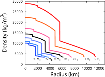
Figure 1: Radial density profiles for 0.1, 0.2, 0.5, 1, 2, 5, 10 $M_{\oplus}$ planets (with inner core of 6 wt% of each core) obtained by our model in the nominal case.

The compositions are assumed as olivine and $\gamma$-spinel for upper mantle, perovskite and post-perovskite for lower mantle, Fe and FeS for outer core, and Fe for inner core with the properties given in Table 1. As temperature decreases, the inner solid core grows and sulfur moves from the inner core to the outer core (see section 2.2). In general, the inner core growth changes the volume of the whole core, because the parameters, $\rho_{0},K_{0}$ and $K_{0}^{\prime}$, are different between Fe and FeS. However, since we numerically found that the volume change of the whole core is very small, we neglect it. Figure 1 shows the result of numerical calculation of the density profile for 0.1 to 10 Earth-mass planets. This result is different in the radii of the core and the mantle from the results by Valencia et al. (2006) and Sotin et al. (2007) by a few %, which may be due to different choice of parameter values in the EOS. But, this difference does not affect the thermal evolution.

2.2 Thermal evolution of the core

The temperature distribution of the core is determined as follows:

1. The inner solid core: We assume that each part of the inner core memorizes the temperature at which it solidified, because of inefficient heat transfer due to conduction in the solid core.

2. The outer liquid core: We assume that the liquid core has an adiabatic temperature distribution by vigorous convection.

3. Time evolution: The radius of the inner core and the temperature at the CMB is determined by total energy of the inner and outer cores as described below, and the total energy is given as a function of time with integrating heat flux at the CMB.

The adiabatic temperature gradient in the outer core is given by (Sohl & Spohn, 1997; Yukutake, 2000; Valencia et al., 2006)

$$\frac{\partial{T}}{\partial{r}}=\frac{\rho g\gamma_{G}}{K_{s}}T,$$ (4)

where $\gamma_{G}$ and $K_{s}$ are Grüneisen parameter and bulk modulus of the liquid core. Depth variation of $\gamma_{G}$ is calculated as $\gamma_{G}=\gamma_{G0}(\rho_{0}/\rho)^{q}$ (the parameter values used are summarized in Table 1). The density at 0 pressure $\rho_{\rm 0OC}$, bulk modulus $K_{\rm 0OC}$, and its pressure derivation $K^{\prime}_{\rm 0OC}$ of the outer core are given by impurity concentration $x_{{\rm S}}$ as:

$$x_{{\rm FeS}}=x_{{\rm S}}\frac{Z_{{\rm Fe}}+Z_{{\rm S}}}{Z_{{\rm S}}}$$ (5)

$${\rho_{0}}_{{\rm OC}}=\left(\frac{1-x_{{\rm FeS}}}{\rho_{{\rm Fe}}}+\frac{x_{{\rm FeS}}}{\rho_{{\rm FeS}}}\right)^{-1}$$ (6)

$${K_{0}}_{{\rm OC}}=\frac{1}{{\rho_{0}}_{{\rm OC}}}\frac{1}{\frac{1-x_{{\rm FeS}}}{\rho_{{\rm Fe}}}\frac{1}{K_{{\rm Fe}}}+\frac{x_{{\rm FeS}}}{\rho_{{\rm FeS}}}\frac{1}{K_{\rm FeS}}}$$ (7)

$${K^{\prime}_{0}}_{{\rm OC}}=-1+{\rho_{0}}_{{\rm OC}}{K_{0}}_{{\rm OC}}\left(\frac{1-x_{{\rm FeS}}}{\rho_{{\rm Fe}}}\frac{1+K^{\prime}_{{\rm Fe}}}{K^{2}_{{\rm Fe}}}+\frac{x_{{\rm FeS}}}{\rho_{{\rm FeS}}}\frac{1+K^{\prime}_{{\rm FeS}}}{K^{2}_{{\rm FeS}}}\right),$$ (8)

where $x_{\rm Fe}$, $x_{{\rm FeS}}$, $Z_{{\rm Fe}}$, and $Z_{{\rm S}}$ are mass fraction of Fe and FeS, molar weights of Fe and S, respectively.

The inner core nucleation decelerates cooling of the core by release of gravitational energy due to the change in the density distribution and by release of latent heat (Stevenson et al., 1983; Gubbins et al., 2004). The light elements are kicked into the outer core, resulting in depression of a melting point of the outer core (Stevenson et al., 1983; Yukutake, 2000). The boundary between inner and outer cores is located at the intersection between adiabatic and melting curves in the core. We use a Lindeman’s equation for the melting curve of pure iron,

$$\Gamma(\rho)=\Gamma_{0}\left(\frac{\rho_{0}}{\rho}\right)^{2/3}\exp\left\{\frac{2\gamma_{0}}{q}\left[1-\left(\frac{\rho_{0}}{\rho}\right)^{q}\right]\right\}.$$ (9)

We also consider the depression of a melting point by concentration of light elements. We define the melting point of Fe-FeS alloy as

$$T_{\rm melt}=(1-2x_{\rm S})\Gamma(\rho),$$ (10)

and the factor $(1-2x_{\rm S})$ expresses the depression of the melting point due to dissolution of light elements (Usselman, 1975; Stevenson et al., 1983). Assuming that the outer core is well mixed by convection,

$$x_{\rm S}=x_{\rm 0S}\frac{M_{{\rm c}}}{M_{{\rm c}}-M_{{\rm ic}}},$$ (11)

where $M_{{\rm ic}}$ and $M_{\rm c}$ are the inner core mass and total mass of the inner and outer cores and $x_{\rm 0S}$ is the initial impurity concentration. In the nominal case, we adopt $x_{\rm 0S}=0.1$.

Given the inner core radius, we can calculate the total energy of the core ($E_{\rm core}$) which is sum of the gravitational energy ($E_{g}$), latent heat ($E_{l}$), and thermal energy ($E_{th}$). As described above, the temperature at the CMB is given as a function of the radius of the inner core. As a result, we can obtain $E_{\rm core}$ as a function of the temperature at the CMB. Conversely, the radius of the inner core and the temperature at the CMB are given as a function of $E_{\rm core}$.

The energies are given by

$$\begin{array}[]{ll}E_{g}&{\displaystyle=-\int^{r_{{\rm ic}}}_{0}4\pi r^{3}\rho_{{\rm ic}}(r)g_{{\rm ic}}(r)dr-\int^{r_{{\rm c}}}_{r_{{\rm ic}}}4\pi r^{3}\rho_{{\rm oc}}(r)g_{{\rm oc}}(r)dr,}\\ E_{l}&=LM_{ic},\\ E_{th}&{\displaystyle=\int^{r_{c}}_{0}4\pi r^{2}\rho(r)C_{p}(r)T(r)dr,}\end{array}$$ (12)

where $L$ is the latent heat released by solidification of unit mass of iron, which is assumed to be constant of $1.2\times 10^{6}$ J/kg (Anderson & Duba, 1997), and not to depend on the impurity concentration in the outer core, and $C_{p}$ is specific heat with constant pressure. Both the gravitational energy and the latent heat are released after the inner core starts to solidify. Gravitational energy is also released by thermal contraction, which will be discussed in section 2.6. The total energy $E_{\rm core}$ decreases with the rate that is equal to the heat flux at the bottom of the mantle (see section 2.3). Detailed calculations of the energies are given in Appendix C.

2.3 Heat transfer throughout mantle

The mantle is cooled by irradiation from the planetary surface and heated by heat flow from the core and internal radioactivity (see below). The heat transfer equation is:

$$\rho C_{p}\frac{\partial{T}}{\partial{t}}=\frac{1}{r^{2}}\frac{\partial{{}}}{\partial{r}}\left\{r^{2}k_{c}\left(\frac{\partial{T}}{\partial{r}}\right)+r^{2}k_{v}\left[\left(\frac{\partial{T}}{\partial{r}}\right)-\left(\frac{\partial{T}}{\partial{r}}\right)_{s}\right]\right\}+\rho Q,$$ (13)

where $k_{c}$ is thermal diffusion coefficient, $Q$ is radioactive heat production rate, $(\partial T/\partial r)_{s}$ is the adiabatic temperature gradient, and the first and second terms in the right hand side represent conductive and convective fluxes.

To evaluate the convective flux in the mantle, we use the astrophysical mixing length theory (MLT) modified for solid planets (Sasaki & Nakazawa, 1986; Abe, 1995; Senshu et al., 2002; Kimura et al., 2009, and references therein), rather than the conventional parameterized convection model (PCM; e.g., Sharpe & Peltier, 1979) or the commonly used boundary layer theory (BLT; e.g., Stevenson et al., 1983).

The PCM is very simple (Appendix A). However, it uses the values of $k_{c}$ and Rayleigh number $Ra$ that represents the whole mantle, which are difficult to evaluate for real mantle because of huge spatial variation of the mantle viscosity. As a result, although the PCM can be applied to study overall trend of thermal evolution, it may not be accurate enough for evaluation of heat flux across the CMB ($F_{\rm CMB}$), which we are concerned with in the present paper. In the BLT, since the heat flux is expressed by quantities only in the thermal boundary layer (Appendix A), the BLT has better resolution for evaluation of $F_{\rm CMB}$. Since the modified MLT also uses local values of physical quantities, it quantitatively agrees with the BLT for wide range of parameters, while the PCM does not agree with the BLT and the MLT for the cases in which viscosity variation is large in the mantle, as shown in Appendix A. As explained below, since the MLT is more easily to be applied for super-Earths, we use the MLT.

In the early Earth, the upper/lower mantle boundary could have worked as a barrier for convection (Honda et al., 1993). Tentative stagnancy at the upper/lower mantle boundary is also suggested for some subduction slabs in the present Earth (Wortel & Spakman, 2000). The density overturn at melt/solid boundary in deep magma ocean in the early Earth may have also worked as the barrier (Labrosse et al., 2007). In super-Earths, post-post perovskite transition in deep mantle at high pressure could also work as a barrier (Umemoto et al., 2006).

As explained below, the modified MLT is easily applied for mantle convection with barriers, without tuning of parameters for each barrier. Although most of our calculations in the present paper only consider the surface boundary and CMB (in some runs we consider the upper/lower mantle boundary at spinel-perovskite transition as well), we use the modified MLT for future extensions of calculations with various convection barriers. In the following papers, we will consider the effects of other barriers.

In the MLT, the coefficient for convective heat transfer is given by

$$k_{v}=\left\{\begin{array}[]{cr}\displaystyle 0&\displaystyle{\rm for}\;\left(\frac{\partial{T}}{\partial{r}}\right)>\left(\frac{\partial{T}}{\partial{r}}\right)_{s}\\ \\ \displaystyle\frac{\rho^{2}C_{p}\alpha g\ell^{4}}{\eta}\left[\left(\frac{\partial{T}}{\partial{r}}\right)-\left(\frac{\partial{T}}{\partial{r}}\right)_{s}\right]&\displaystyle{\rm for}\;\left(\frac{\partial{T}}{\partial{r}}\right)<\left(\frac{\partial{T}}{\partial{r}}\right)_{s}\\ \end{array}\right.$$ (17)

where $\eta$ and $\ell$ are viscosity and the mixing length, respectively. Here, the velocity of fluid blobs is evaluated by Stokes velocity rather than free fall velocity in the original MLT, in order to apply the model to low Reynolds number flow in the mantle. In the astrophysical context such as stellar interior, the density scale height is usually adopted as $\ell$. For calculation of thermal evolution of the Earth, it is proposed that a distance ($D$) from the closest barrier such as the CMB or the top of the mantle layer is appropriate for $\ell$ (Sasaki & Nakazawa, 1986; Abe, 1995; Senshu et al., 2002; Kimura et al., 2009, and references therein). The detailed comparison with the PCM and BLT in Appendix A shows that $\ell=0.82D$ is the best choice. We adopt $\ell=0.82D$ for all the runs in the present paper.

With this choice, as approaching a barrier, $k_{v}$ rapidly decreases in proportion to $\ell^{4}$ and the conductive term dominates in Eq. (13). As a result, thermal boundary layers, in which the conductive heat transfer dominates, are automatically represented. Thereby, the modified MLT is easily applied for calculation for thermal evolution of the proto-Earth or super-Earths.

The mantle viscosity is discussed in section 2.5. The heat flux and temperature at the CMB determined from the calculation of the mantle heat transfer is used as a boundary condition for thermal evolution of the mantle. The total energy in the core is interpolated from the result of section 2.2. It decreases with time, according to the calculated heat flux at the CMB.

2.4 Internal heat source

For thermal evolution of terrestrial planets on geological timescales, long-lived radiogenic elements (⁴⁰K, ²³²Th, ²³⁵U, and ²³⁸U) are important heat sources in the mantle. The estimated amounts of these elements in the Earth are compiled in table 2 (van Schmus, 1995). Here we assume the same abundances of the radiogenic elements in the mantle in super-Earths as those in the Earth and that the elements are distributed uniformly throughout the mantle. The heat production rate at time $t$, $Q(t)$, is given by $Q(t)=HU\exp(-\lambda(t-t_{\oplus}))$ where $U$, $H$, $t_{\oplus}$ and $\lambda$ are the abundance, heat production rate, and decay constant of the element, respectively.

2.5 Temperature and pressure dependency of mantle viscosity

The mantle viscosity is one of the most important physical parameters to simulate thermal evolution, since it determines the heat transfer efficiency in the mantle (see Eqs. [13] and [17]). The viscosity sensitively depends on temperature and pressure, and both of temperature and pressure widely vary throughout the mantle. Here, we adopt Arrhenius type formulation for temperature- and pressure-dependent viscosity model (Ranalli, 2001):

$$\eta(T,P)=\frac{1}{2}\left[\frac{1}{B^{1/n}}\exp\left(\frac{E^{*}+PV^{*}}{nRT}\right)\right]\dot{\epsilon}^{(1-n)/n},$$ (18)

where $R$, $\dot{\epsilon}$, $n$, $B$, $E^{*}$ and $V^{*}$ are universal gas constant, strain rate, creep index, Barger coefficient, activation energy, and activation volume of mantle, respectively. We use different values of these parameters for upper and lower mantles. The mineral properties we use are listed in Table 3. Note that the prescription for the mantle viscosity may include uncertainty. The formula is based on the theoretical rate equation for creep law of rocks. In this formula, the most important parameter to study thermal evolution of super-Earths is the activation volume ($V^{*}$), since $V^{*}$ determines the dependence of the viscosity on pressure and the pressure in the mantle can be increased by orders of magnitude as the planetary mass increases. The activation volume is related to atomic volume, but the exact values under extremely high pressure is not well determined. In the nominal case, we use $V^{*}=10\times 10^{-6}\mathrm{m^{3}mol^{-1}}$, but we also test a smaller value of $V^{*}=3\times 10^{-6}\mathrm{m^{3}mol^{-1}}$. In section 3.4, we will discuss how the conclusion in the present paper depends on a formula for the viscosity.

2.6 Release of gravitational energy by thermal contraction

Although the thermal contraction is negligible for physical radius, the gravitational energy released by the thermal contraction cannot be neglected (it is about 50kJ/kg for 100K change of the core in an Earth-mass planet). In our model, the released energy is regarded as increase in the specific heat of the core (Yukutake, 2000):

$$\Delta C_{p}=\frac{\alpha P}{\rho}.$$ (19)

The gravitational energy released by thermal contraction is more effective in deeper regions. For an Earth-mass planet, $\Delta C_{p}/C_{p}$ is as large as 50% at the CMB in our calculation.

2.7 Initial conditions

Initial temperature distribution in the mantle is determined by the procedure following Yukutake (2000), as illustrated in Fig. 2: (1) An adiabat is drawn from the bottom of the surface boundary layer with 1500 K down to the top of the boundary layer at the CMB (the obtained tentative temperature is denoted by $T_{2}$), assuming efficient thermal convection, (2) the initial temperature at the bottom of the CMB is assumed to be $T_{\rm CMB}=T_{2}+\Delta T_{\rm CMB}$, where $\Delta T_{\rm CMB}$ is determined by step 6, (3) the adiabat is drawn from the CMB with temperature $T_{\rm CMB}$ to the surface, (4) the initial temperature distribution in the mantle is given by the average of the two adiabats obtained by steps 1 and 3, (5) core temperature is determined by the procedure given in section 2.2 with $T_{\rm CMB}$, and (6) the amount of $\Delta T_{\rm CMB}$ ($\sim 1000$K) is determined by the requirement that the predicted surface heat flux and inner core radius for an Earth-mass planet are comparable to the observed values for the present Earth. We use this value for all the cases with various planetary masses. Note that the temperature distribution is quickly relaxed to an equilibrium distribution, as long as we use the initial conditions created by the above procedures.

2.8 Simulation parameters

We summarize parameters for the “nominal” case:

• Boundary conditions

  • surface temperature: $T_{\rm surf}=300$K

  • a mass ratio between mantle and core: $\zeta_{\rm m/c}=7:3$

  • the CMB is a barrier for convection, while convection penetrates the upper/lower mantle boundary

• Initial conditions

  • impurity fraction: $x_{\rm 0S}=0.1$

• Rheological conditions

  • activation volume: $V^{*}=10\times 10^{-6}\mathrm{m^{3}mol^{-1}}$

We first investigate planetary mass dependence for planets with the above nominal parameters. For Earth-mass planets, we adopt $\Delta T_{\rm CMB}=1000$K in most runs, because the nominal case with $\Delta T_{\rm CMB}=1000$K reproduces the present Earth. We also systematically study dependences of the results on $\Delta T_{\rm CMB}$, because $\Delta T_{\rm CMB}$ is not well determined. In some runs, the upper/lower mantle boundary is treated as a barrier for convection. We also carry out calculations with different values of $T_{\rm surf}$, $\zeta_{\rm m/c}$, and $x_{\rm 0S}$ to reproduce the results that are consistent with the current magnetic fields of Mercury, Venus, and Mars in Appendix B (we do not systematically survey the dependences on these parameters).

2.9 Definition of lifetime of planetary intrinsic magnetic field

To drive dynamo action, liquid metallic core must be in active convection state. Following Stevenson et al. (1983), we adopt the threshold heat flux in the core for generation of dynamo action (conducted heat flux along the core adiabatic thermal structure) as,

$$F_{\rm crit}=k_{c}\left(\frac{\partial T_{\rm CMB}}{\partial r}\right)_{S}=k_{c}\frac{\rho g\gamma_{G}}{K_{s}}T_{{\rm CMB}}.$$ (20)

We define the lifetime of magnetic field as a period during which the core heat flux exceeds the threshold value.

3 Numerical Results

3.1 Thermal evolution of the Earth

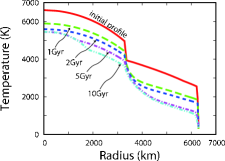
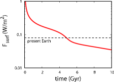
(c)                                               (d)

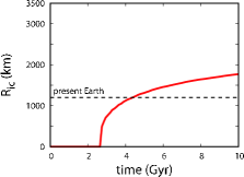
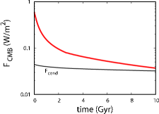
Figure 3: Time evolution of (a) the temperature profile, (b) the surface heat flux, (c) the inner core radius and (d) the heat flux through CMB for an Earth-mass planet with $\Delta T_{CMB}=1000K$. (a)Time evolution of internal temperature distribution in the case of $\Delta T_{CMB}=1000K$ with 1 $M_{\oplus}$. The planet radius of 6385km and core radius of 3375km. The surface heat flux declines to $\sim 0.08$ ${\rm Wm^{-2}}$ and the inner core grows up to 1200 km at 4.5 Gyr after, which is nearly equal to the present observed value of the inner core radius of the Earth. The core heat flux monotonically decreases with time but its time derivative discontinuously changes at the initiation of the inner core at around 2.2 Gyr. The solid curve represents the threshold flux ($F_{\rm cond}$) to maintain dynamo activity in the outer core (Eq. [20]).

We now show the evolution of temperature distribution calculated by the procedures in section 2. Figure 3a shows the evolution of thermal structure of an Earth-mass ($M=1M_{\oplus}$) planet for the nominal case. Cooling of the mantle slows down with time, since the decrease in temperature enhances the mantle viscosity (eq. [18]) and hence depresses the efficiency of heat transfer in the mantle. This implies that the initial mantle temperature distribution hardly affects the thermal evolution on timescales longer than Gyr, as long as the initial temperature is high enough (Stevenson et al., 1983). However, since the core works as a heat bath for the mantle, the initial $T_{\rm CMB}$ would affect the thermal evolution of the mantle.

Figures 3b, c and d show the time evolution of the surface heat flux ($F_{\rm surf}$), the heat flux across the CMB ($F_{\rm CMB}$) and the inner core radius ($R_{\rm ic}$), respectively, in the nominal case. We adopt $\Delta T_{\rm CMB}=1000$K. The inner core emerges at 2.2 Gyr. Its radius reaches 1200km at 4.5Gyr that agrees with the observed value of the present Earth, as expected. With higher/lower values of $T_{\rm CMB}$, the inner core radius at 4.5Gyr is smaller/larger. The growth rate decreases with time, because not only geometric effect but also the increase in impurity concentration in the outer core depresses the melting point of the outer core. After the emergence of the inner core, the heat flux reduction becomes more slowly because the inner core growth releases gravitational energy and latent heat that work as internal heat sources. The heat flux remains larger than the critical value given by Eq. (20), which is expressed by the dot-dashed line in Fig. 3d, during first 12 Gyr and the lifetime of dynamo activity is expected to be 12 Gyr for this nominal case.

Some paleomagnetism data suggests that the magnetic field of the Earth is enhanced to be the present level at $\sim 2$ Gyr (e.g., Hale, 1987). It might be due to formation of the inner core because nucleation of the inner core provides additional heat source. Paleomagnetism data may include a large uncertainty. If more detailed data is provided, it will constrain the condition of generation of intrinsic magnetic field.

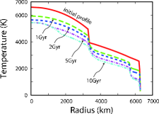
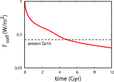
(c)                                               (d)

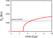
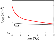
Figure 4: Same figures as Figs. 3 except for two-layered mantle convection model with $\Delta T_{\rm CMB}=$1000K.

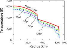
(c)                                               (d)

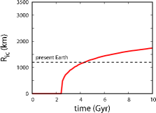
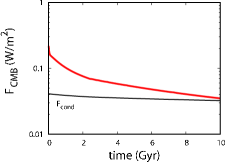
Figure 5: Same figures as Figs. 3 except that two-layered mantle convection model with $\Delta T_{CMB}=800K$ is considered instead of one-layered model with $\Delta T_{\rm CMB}=$1000K.

Figures 4 and 5 show the results of the two-layer convection. In this calculation, we set the upper/lower mantle boundary as a barrier for convection. The other boundary conditions and the model parameters are the same as those in the nominal case. The mixing length is shorter in the entire regions of mantle and cooling is slower than in the one-layer case. As is shown in Figures 4, if we adopt initial $\Delta T_{\rm CMB}=1000$K as in the case of one-layer convection, the inner core can not grow to 1200km because of the low heat transfer efficiency of the layered convection and core temperature is somewhat higher than that obtained by the one-layer convection. We also carried out a calculation with initial $\Delta T_{\rm CMB}=800K$. Figure 5a shows the evolution of thermal profile. A thermal boundary layer at upper/lower mantle boundary is clearly established. Because the lower initial $\Delta T_{\rm CMB}$ is compensated with the inefficient two-layer convection, evolution of heat flux through CMB ($F_{\rm CMB}$) and lifetime of magnetic field (11Gyr in this case) are similar to those in the one-layer convection case.

If the two-layer convection is assumed only in the Archean and Hadean ($t<2$Gyr), with the same initial $\Delta T_{\rm CMB}$ (1000K) the surface heat flux at 4.5Gyr is $F_{\rm surf}\sim 0.12{\rm Wm^{-2}}$, which is somewhat higher than the observed value ($\sim 0.09{\rm Wm^{-2}}$), since the thermal energy beneath upper/lower mantle boundary have been stored until 2Gyr and then supplied to upper mantle after 2Gyr. However, the evolution of $F_{\rm CMB}$ is not so different between one- and two-layer convection. The lifetime of magnetic field is about 12 Gyrs.

Thus, if we tune the initial $\Delta T_{\rm CMB}$ with the present observed values of $F_{\rm surf}$ and $R_{\rm ic}$, the expected lifetime of magnetic field is not affected by the mode (one-layer or two-layer) of mantle convection.

3.2 Thermal evolution of Mercury, Venus, and Mars

The existence of the magnetic field for Mercury and early decay of the magnetic field for Venus and Mars were addressed by Stevenson et al. (1983), using the box model with different parameter values such as surface temperature and a mantle-core mass ratio from those in the nominal case. The validity of these parameter values is discussed in Appendix B. Adopting the same parameter values as Stevenson et al. (1983), we have performed simulations for Mercury, Venus, and Mars with our model. As discussed in Appendix B, our model produces the results that are not inconsistent with the magnetic activity of Mercury, Venus, and Mars.

3.3 Thermal evolution of super-Earths

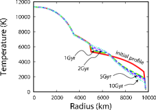
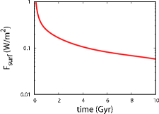
(c)                                               (d)

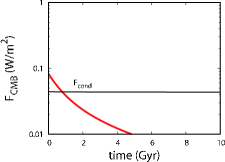
Figure 6: Same figures as Figs. 3 except for $M_{p}=5M_{\oplus}$.

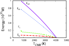
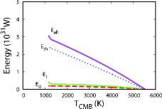
$5M_{\oplus}$                                            $10M_{\oplus}$

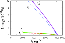
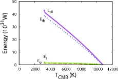
Figure 15: Individual core energies as a function of $T_{\rm CMB}$ for the nominal case with $M=1,2,5,10M_{\oplus}$ and $x_{\rm 0S}=0.1$. Dashed, dotted, and dot-dashed curves represent gravitational energy, latent heat, and thermal energy, respectively. Solid curve shows the total energy. The gradient of total energy corresponds to the specific heat of the core.

For super-Earths, we use the nominal parameters (the surface temperature is 300K and the mantle/core mass ratio is 7:3), assuming that their orbits are nearly circular and in habitable zones. We also assume one-layer convection throughout the mantle. Detailed study on the effects of phase transitions is left to future works. Figure 6a shows evolution of temperature distribution for a planet with mass $M_{p}=5M_{\oplus}$. Compared with the case of $M_{p}=1M_{\oplus}$ in Figure 3a, a thicker thermal boundary layer is established on the CMB within first few Gyrs, since the viscosity of the bottom of the mantle is higher. The increase in the viscosity due to higher pressure dominates the decrease due to higher temperature (Eq. [18]). Thus, $F_{\rm CMB}$ is lower than the case of $M_{p}=1M_{\oplus}$ (Figs. 6b and 3b). On the other hand, the effective heat capacity rapidly increases with $M_{p}$. Figures 15 in Appendix C show that for fixed $T_{\rm CMB}$, thermal energy $E_{\rm th}\propto M_{p}^{2}$, while the core surface area $S_{\rm core}$ increases with $M_{p}$ only weakly ($S_{\rm core}\propto M_{p}$). Therefore, the core for higher $M_{p}$ cools much more slowly. It is shown that $R_{\rm ic}$ does not grow at all for 10Gyr. On the other hand, $F_{\rm surf}$ is not so different from that in the case of $M_{p}=1M_{\oplus}$. The heat bath of surface heat flow is radiogenic elements in the mantle and that is proportional to $M_{p}$. To balance heat generation and cooling, $F_{\rm surf}$ should be proportional to $M_{p}^{1/3}$, provided $R_{p}\propto M_{p}^{1/3}$. Thereby $F_{\rm surf}$ changes by a factor of only $5^{1/3}\sim 1.7$.

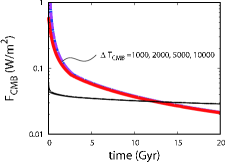
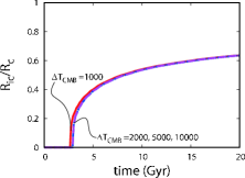
(b)

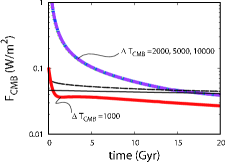
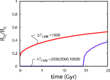
(c)

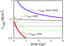
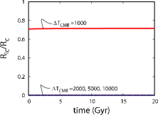
(d)

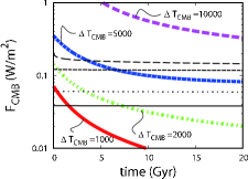
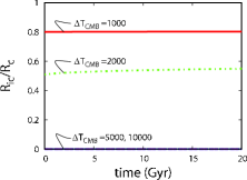
Figure 7: Evolution of the core heat flux (left column) and inner core radius (right column) for $M=$ (a)1, (b) 2, (c) 5, (d) and 10 $M_{\oplus}$ with various initial $\Delta T_{\rm CMB}$. In the left column, $F_{\rm crit}$ for each $\Delta T_{\rm CMB}$ is expressed by thinner line with the same type. Some lines with different initial $\Delta T_{\rm CMB}$ are overlapped by each other. For these parameters, the initial conditions do not affect the evolution since self-regulation of mantle heat transfer works due to temperature dependence of the mantle viscosity. Inner cores never nucleate in the cases of $\Delta T_{\rm CMB}=2000,5000,$ and $10000$K for $M_{p}=5M_{\oplus}$ and $\Delta T_{\rm CMB}=5000$ and 10000K for $M_{p}=10M_{\oplus}$.

As discussed in the above, thermal evolution of super-Earths differs from that of Earth-mass planets in many aspects. Here, we focus on evolution of heat flux through CMB, $F_{\rm CMB}$, and inner core radius, $R_{\rm ic}$, in order to study magnetic activity of super-Earths. Figures 7 show the evolution of $F_{\rm CMB}$ (left column) and $R_{\rm ic}$ (right column) with various initial $\Delta T_{\rm CMB}$ for the case of (a) $M_{p}=1M_{\oplus}$, (b) $2M_{\oplus}$, (c) $5M_{\oplus}$, and (d) $10M_{\oplus}$. Solid, dot, dashed, and long-dashed lines represent the results with initial $\Delta T_{\rm CMB}=1000$K, 2000K, 5000K and 10000K, respectively. In all cases, $V^{*}=10\times 10^{-6}{\rm m^{3}/mol}$.

The results in the left column show that $F_{\rm CMB}$ is generally higher for higher initial $\Delta T_{\rm CMB}$. The dependence is more pronounced for relatively large $M_{p}$ cases. For $M_{p}=1~{}M_{\oplus}$, the dependence is very weak. We found the dependence is also very weak for $M_{p}<1~{}M_{\oplus}$. For $M_{p}\hskip 4.30554pt^{<}{}_{\sim}\hskip 4.30554pt1~{}M_{\oplus}$, the temperature dependence of the mantle viscosity (Eq. [18]) dominates over the pressure dependence. Then, $F_{\rm CMB}$ is high when the core temperature is high, and $F_{\rm CMB}$ declines as the core cools. Thus, the heat flux is self-regulated to be quickly relaxed independent of the initial values. On the other hand, as will be shown later, when $\Delta T_{\rm CMB}\hskip 4.30554pt^{<}{}_{\sim}\hskip 4.30554pt1000(M_{p}/M_{\oplus})$, the pressure dependence is more effective. Then, the self-regulation does not work and the dependence of $F_{\rm CMB}$ on initial $\Delta T_{\rm CMB}$ is retained for more than 20 Gyrs. The threshold flux for driving dynamo action is marked by an black lines in each case. The decline of the threshold value is due to decrease of core surface temperature (Eq. [20]). The duration for $F_{\rm CMB}>F_{\rm crit}$ determines lifetime of magnetic field generation.

Papuc & Davies (2008) obtained $F_{\rm CMB}\propto M_{p}^{2/3}$, whereas our results shows $F_{\rm CMB}\propto M_{p}$ provided that $\Delta T_{\rm CMB}$ is sufficiently high. The difference may come from the assignment of specific heat of the core. Papuc & Davies (2008) assumed constant specific heat of the core, $C_{p}=1000{\rm JkgK^{-1}}$ for all sized planets. As we discussed in section 2.6, however, thermal contraction results in increase in the effective $C_{p}$ and the effect is more pronounced for larger $M_{p}$. In our calculations that include this effect, the core tends to cool less efficiently and the dependency of $F_{\rm CMB}$ on $M_{p}$ is stronger than that obtained by Papuc & Davies (2008).

The right column shows the growth of inner solid cores for $\Delta T_{\rm CMB}=1000,2000,5000$ and 10000K. In the case of $M_{p}=1~{}M_{\oplus}$, an inner core is nucleated at 2-3 Gyrs, almost independent of initial $\Delta T_{\rm CMB}$, since the core cooling is self-regulated. For $M_{p}=2M_{\oplus}$, the inner core growth depends on $\Delta T_{\rm CMB}$ for $\Delta T_{\rm CMB}\hskip 4.30554pt^{>}{}_{\sim}\hskip 4.30554pt2000$K. For such high $\Delta T_{\rm CMB}$, since the core has larger thermal energy initially and the heat flux is not self-regulated, it takes more time for the core temperature to become below the nucleation temperature. For $M_{p}\hskip 4.30554pt^{>}{}_{\sim}\hskip 4.30554pt5M_{\oplus}$, core hardly cools on 20 Gyrs, the inner core does not grow from the initial state. In these cases the inner core size is determined by a relationship between adiabatic curve and melting curve of iron. The inner core of super-Earths ($M_{p}>M_{\oplus}$) have never nucleated for $\Delta T_{\rm CMB}=10000$K. For massive planets, the increase in the viscosity due to higher pressure is overcome only by very high initial temperature. The high $\Delta T_{\rm CMB}$ also delays nucleation of the inner solid core. As a result, there is trade off between heat flux and inner core growth through the relation between melting point of iron core and temperature- and pressure-dependency of mantle viscosity.

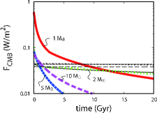
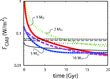
(c)                                               (d)

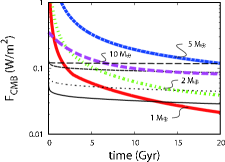
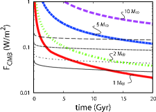
Figure 8: Evolution of the core heat flux for $\Delta T_{\rm CMB}$ = (a)1000K, (b) 2000K, (c) 5000K, (d) 10000K with $M_{p}=1,2,5,10M_{\oplus}$, respectively.

Figures 8 show dependence of evolution of $F_{\rm CMB}$ on $M_{p}$ for fixed values of $\Delta T_{\rm CMB}$. For $\Delta T_{\rm CMB}=1000$K, we have already mentioned that $F_{\rm CMB}$ is rather lower for $M_{p}=5M_{\oplus}$ than for $M_{p}=M_{\oplus}$ (Figs. 6b and 3b), because the increase in the viscosity due to higher pressure dominates the decrease due to higher temperature for $M_{p}=5M_{\oplus}$. This trend is clearly shown in Fig. 8a.

However, this is not always the case. If the core temperature is high enough (in other words, $\Delta T_{\rm CMB}$ is high enough), or if pressure is low enough ($M_{p}$ is small enough), the viscosity should decrease with increase in $M_{p}$ due to the temperature effect. For $\Delta T_{\rm CMB}=10000$K (Fig. 8d), $F_{\rm CMB}$ is approximately proportional to $M_{p}$. Even for $\Delta T_{\rm CMB}=1000~{}\mbox{K}$, $F_{\rm CMB}$ increases with $M_{p}$ for low mass regime ($M_{p}<1M_{\oplus}$). Thus, $F_{\rm CMB}$ has a peak at some value of $M_{p}$ for a given value of $\Delta T_{\rm CMB}$. Figures 8b and c show that the critical planet mass ($M_{p,c}$) at which $F_{\rm CMB}$ takes the maximum value is $2M_{\oplus}$ for $\Delta T_{\rm CMB}=2000$K and $5M_{\oplus}$ for 5000K. We empirically found that

$$M_{p,c}\simeq\frac{\Delta T_{\rm CMB}}{1000{\rm K}}M_{\oplus}.$$ (21)

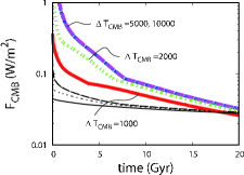
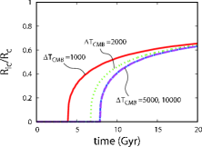
(b)

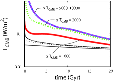
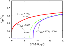
(c)

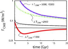
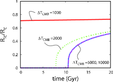
(d)

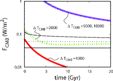
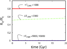
Figure 9: Same as Fig. 7except $V^{*}=3\times 10^{-6}{\rm m^{3}mol^{-1}}$

Since the mantle viscosity depends on the activation volume, $V^{*}$ (Eq. [15]), and the values of $V^{*}$ may have uncertainty at high pressure, we also performed calculations with a smaller value of $V^{*}$. Figures 9 show the results with $V^{*}=3\times 10^{-6}{\rm m^{3}mol^{-1}}$. Due to the weakened pressure effect, $M_{p,c}$ is increased by a factor of a few. In Figures 9, the viscosity is artificially increased (Eq. [15] by a factor of 6000) in order to compensate the smaller value of $V^{*}$ and reproduce Earth’s observed values. Note that the artificial increase does not affect $M_{p,c}$.

The critical planetary mass $M_{p,c}$ is approximately derived by the $M_{p}$-dependence of the mantle viscosity at CMB. Since we empirically found that $P_{\rm CMB}\sim(M_{p}/M_{\oplus})P_{\oplus{\rm CMB}}$ and $T_{\rm CMB}\sim 5\Delta T_{\rm CMB}$, Eq. (18) is reduced to

$$\eta_{\rm CMB}(M_{p},T_{\rm CMB})\propto\exp\left(\frac{E^{*}+\left(\frac{M_{p}}{M_{\oplus}}\right)P_{\oplus}V^{*}}{nRT_{\rm CMB}}\right).$$ (22)

When the argument of exponential is larger than unity, the viscosity rapidly increases with $M_{p}$ to depress $F_{\rm CMB}$, because $F_{\rm CMB}\propto\eta^{-1/3}$. For $M_{p}<M_{p,c}$, we found that $F_{\rm CMB}\propto M_{p}$. When the argument exceeds some critical value ($C>1$), the viscosity enhancement eventually overwhelms the factors for the positive $M_{p}$-dependence of $F_{\rm CMB}$. Thus, $M_{p,c}$ is given by the value of $M_{p}$ with which the argument of exponential is $\simeq C$,

$$M_{p,c}\simeq\frac{5nCR\Delta T_{\rm CMB}-E^{*}}{V^{*}}\frac{M_{\oplus}}{P_{\oplus{\rm CMB}}}$$

$$\simeq\frac{5nCR\Delta T_{\rm CMB}}{V^{*}}\frac{M_{\oplus}}{P_{\oplus{\rm CMB}}}$$

$$\sim\frac{C\Delta T_{\rm CMB}}{10000K}\left(\frac{V^{*}}{10\times 10^{-6}{\rm m^{3}mol^{-1}}}\right)^{-1}M_{\oplus},$$ (23)

which explains the dependences on $\Delta T_{\rm CMB}$ and $V^{*}$ that we found numerically. (If we adopt $C\sim 10$, the numerical factor is also explained.)

3.4 Lifetime of intrinsic magnetic fields

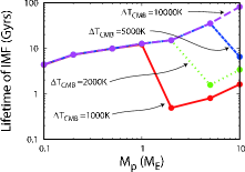
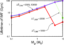
Figure 10: Lifetime of magnetic fields as a function of planetary mass ($M_{p}$) with various $\Delta T_{\rm CMB}$ for (a) $V^{*}=10\times 10^{-6}{\rm m^{3}mol^{-1}}$ and (b) $V^{*}=3\times 10^{-6}{\rm m^{3}mol^{-1}}$.

The lifetime of the intrinsic magnetic fields is calculated for $\Delta T_{\rm CMB}=1000,2000,5000$ and 10000 K with a fixed value of $V^{*}=10\times 10^{-6}{\rm m^{3}mol^{-1}}$. The results are summarized in Fig. 10. It is clearly shown that the lifetime declines for $M_{p}\hskip 4.30554pt^{>}{}_{\sim}\hskip 4.30554ptM_{p,c}$ by the increase in the mantle viscosity due to the pressure effect that we discussed in details in the previous subsection. The results for $V^{*}=3\times 10^{-6}{\rm m^{3}mol^{-1}}$ show a similar property.

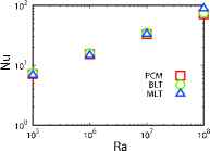
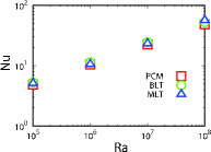
(c)                                       (d)

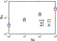
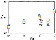
Figure 13: Temporal averaged Nusselt numbers obtained by PCM, BLT and MLT models. The viscosity is changed from the bottom to the top with the ranges of (a) $\Delta\eta$= 10, (b) $10^{2}$, (c) $10^{3}$ and (d) $10^{4}$, respectively.

In Fig. 10, the lifetime weakly increases with $M_{p}$ for $M_{p}\hskip 4.30554pt^{<}{}_{\sim}\hskip 4.30554ptM_{p,c}$. The dependence is explained as follows. The lifetime is approximately given by $\tau_{\rm life}\sim E_{\rm th}/(S_{\rm CMB}F_{\rm CMB})$, where $E_{\rm th}$ is thermal energy of the core and $S_{\rm CMB}$ is surface area of the core. According to our calculation, $S_{\rm CMB}\propto M_{p}^{1/2}$ rather than $M_{p}^{2/3}$ due to self-compression. Figures 7 and 13 show that $F_{\rm CMB}\propto M_{p}$ and $E_{\rm th}\propto M_{p}^{2}$ for a fixed $T_{\rm CMB}$. As we mentioned in section 3.3, $T_{\rm CMB}\sim 5\Delta T_{\rm CMB}$. Thus, for a fixed $\Delta T_{\rm CMB}$, it is predicted that $\tau_{\rm life}\sim E_{\rm th}/(S_{\rm CMB}F_{\rm CMB})\propto M_{p}^{2-1/2-1}=M_{p}^{1/2}$, which is consistent with the numerical results in Fig. 10.

When $M_{p}>M_{p,c}$, the higher mantle viscosity due to the effect of higher pressure significantly depresses heat transfer at the bottom of the mantle. The suppressed heat flux cannot maintain the vigorous core convection. As a result, the magnetic field lifetime is rather shorter for $M_{p}>M_{p,c}$.

Figure 10 also shows that the lifetime for $M_{p}<M_{\rm p,c}$ does not depend on $\Delta T_{\rm CMB}$ at all. The initial temperature is high enough to overcome the pressure-dependency even for the case of $\Delta T_{\rm CMB}=1000$ K, resulting in the effective self-regulation of $F_{\rm CMB}$. As a result, the lifetime does not depend on the initial value of $\Delta T_{\rm CMB}$.

3.5 Strength of magnetic fields

The strength of magnetic fields is as important as their lifetime to discuss habitability of the planets. Here we evaluate the strength of the magnetic fields, using the scaling law derived by Christensen et al. (2009), For planets with sufficiently rapid spins, Christensen et al. (2009) derived the magnetic strength at the core surface as

$$,B_{c}\sim 0.5\mu_{0}^{1/2}\bar{\rho}_{c}^{1/6}F_{\rm conv}^{1/3},$$ (24)

where $\bar{\rho}_{c}$ is average density of the core and $\mu_{0}$ is permeability. If the magnetic moment is dipole-dominant and the dipole moment is $\propto 1/r^{3}$ (Gaidos et al., 2010), the strength of magnetic dipole at the planetary surface is $B_{\rm surf}=B_{c}(r_{c}/r_{p})^{3}$.

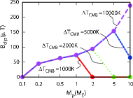
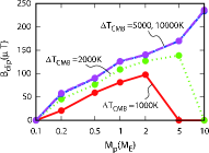
Figure 11: Strength of magnetic fields after 5 Gyr as a function of planetary mass ($M_{p}$) with various $\Delta T_{\rm CMB}$ for (a) $V^{*}=10\times 10^{-6}{\rm m^{3}mol^{-1}}$ and (b) $V^{*}=3\times 10^{-6}{\rm m^{3}mol^{-1}}$.

With $F_{\rm conv}=F_{\rm CMB}-F_{\rm cond}$, we calculated $B_{\rm surf}$ from our simulation results. Figure 11 shows the calculated $B_{\rm surf}$ at $t=5$Gyr for various $M_{p}$ and $\Delta T_{\rm CMB}$. The strength monotonically increases if the initial $\Delta T_{\rm CMB}$ is sufficiently high. The relatively weak dependence ($B\propto M_{p}^{1/3}$) comes from the adopted the scaling law, $B\propto F_{\rm conv}^{1/3}$, and the numerically obtained relation, $F_{\rm CMB}\propto M_{p}$. If $\Delta T_{\rm CMB}$ is not high enough, the pressure effect is dominant and the strength is significantly suppressed for $M_{p}\hskip 4.30554pt^{>}{}_{\sim}\hskip 4.30554ptM_{p,c}$.

4 Conclusion and Discussion

We have developed a numerical model to simulate thermal evolution of various-mass terrestrial planets in habitable zones. The density distribution of the planetary interior is calculated by Vinet EOS taking into account pressure dependence. Using the interior structure model, we calculate heat transfer through mantle, using the astrophysical mixing length theory modified to mantle convection. The modified mixing length theory is easily applied to multi-layer convection that may be dominated convection mode in super-Earths. We have calibrated the modified mixing length theory with the conventional parametrized convection model and the boundary layer theory, in simple one-layer convection cases.

With nominal parameters of surface temperature $T_{\rm surf}=300$K, a mantle-core mass ration $\zeta_{m/c}=7:3$, initial core impurity $x_{\rm 0S}$ of 10 wt%, and initial temperature gap at CMB $\Delta T_{\rm CMB}=1000$K, our model for $M=1M_{\oplus}$ reproduces surface heat flow and inner core radius of the present Earth. With different parameter values suitable for Mercury, Venus, and Mars, our model also reproduces the results that are not inconsistent with present magnetic activity of these planets.

With this model, we calculated thermal evolution of terrestrial planets with mass $M_{p}=0.1$–$10M_{\oplus}$ in habitable zones, using the nominal parameters, to study lifetime of intrinsic magnetic field that is one of the important factors for the planets to be habitable. We found from the numerical calculations that the lifetime is maximized at

$$M_{p,c}\sim\frac{\Delta T_{\rm CMB}}{1000K}\left(\frac{V^{*}}{10\times 10^{-6}{\rm m^{3}mol^{-1}}}\right)^{-1}M_{\oplus},$$ (25)

where $V^{*}$ is activation volume of mantle material. Planets with smaller masses cool more rapidly, so that they cannot maintain core heat flux to generate dynamo long enough. For $M_{p}>M_{p,c}$, the rapid increase in the mantle viscosity caused by high pressure significantly depresses heat transfer throughout the mantle and hence that in the core. As a result, dynamo cannot last long. Although the temperature effect tends to decrease the mantle viscosity as planetary mass becomes large, the pressure effect to increase the viscosity overwhelms the temperature effect for $M_{p}>M_{p,c}$. With the numerically obtained empirical relation, $T_{\rm CMB}\sim 5\Delta T_{\rm CMB}$, we can analytically derive Eq. (25) from the Arrhenius-type formula for the mantle viscosity that we adopt (Eq. [15]).

We found that while the lifetime of magnetic fields does not depend on $\Delta T_{\rm CMB}$ for $M_{p}<M_{p,c}$, it sensitively depends on $\Delta T_{\rm CMB}$ for $M_{p}>M_{p,c}$ because $M_{p,c}\propto\Delta T_{\rm CMB}$ (Eq. [25]). The initial $\Delta T_{\rm CMB}$, that is, the initial temperature profile of planetary interior, is one of the most uncertain parameters, because it highly depends on the processes of planetary formation and differentiation of the planetary interior. As is shown by SPH simulations, if a planet undergoes giant impacts, its metallic core is heated as high as several tens thousands K for $M_{p}\sim 1~{}M_{\oplus}$ (Canup, 2004). On the other hand, if a planet accreted from small planetesimals without giant impacts, the initial temperature profile is determined by the balance between gravitational energy buried by planetesimals and thermal transfer efficiency through rocky mantle. The process includes crystallization of magma ocean and depends on the mechanical property of molten mantle (Abe & Matsui, 1986; Zahnle et al., 1988; Senshu et al., 2002). Thus, to evaluate the lifetime of magnetic fields, in particular for super-Earths that are likely satisfy $M_{p}>M_{p,c}$, detailed analysis for accretion and early thermal evolution of terrestrial planets are needed.

It is also found that higher initial temperature profile delays the inner core nucleation. For super-Earths, in order to maintain magnetic field more than 10 Gyr, the initial temperature has to be high enough to overwhelm the pressure-dependence. However, in that case, the temperature of the core center never reaches its condensation temperature and the inner core cannot grow. Some geo-dynamo simulations suggest that the presence of the inner core stabilizes the dipole moment of geomagnetic field (Sakuraba & Kono, 1999). It is also suggested that because thermally driven convection is not sufficient to drive dynamo action against the ohmic dissipation within the core of Earth (Gubbins et al., 2003), the compositional convection induced by light elements released to the outer core by solidification of the inner core plays an essential role in dynamo generation (Stevenson et al., 1983; Gubbins et al., 2004). Since our results (Figures 6) show that inner core is not nucleated and compositional convection does not occur for $M_{p}\hskip 4.30554pt^{>}{}_{\sim}\hskip 4.30554pt5M_{\oplus}$, dipole magnetic fields of super-Earths might not be stable.

The existence of magnetic field of extrasolar planets could be directly detected by the polarization observation of the photon from transiting planets or detection of H${}_{3}^{+}$ trapped by the magnetic fields in the future. Another possibility of the detection of planetary magnetic field is, although it is indirect, observation of composition of planetary atmosphere or atmospheric tail. If the planet has intrinsic magnetic field, its atmosphere could keep H₂O molecules for long period. Venus may have lost H₂O molecules on a short time scale (Bullock & Grinspoon, 2001). Thus if water series molecules, such as H₂O, H₃O, and HO, were detected in the planetary atmosphere, it would indicate the existence of intrinsic magnetic field, although super-Earths might be able to sustain the H_XO molecules in the atmosphere by their high gravity even without the protection by magnetic fields.

We need to elaborate our thermal evolution model, by considering details of mantle convection mode that is affected by phase transition between $\gamma$-spinel to perovskite (Christensen & Yuen, 1985) at upper/lower mantle. We also should take into account further mineral transitions suggested by ab initio calculations (Umemoto et al., 2006) that may appear in super-Earths, because they may affect internal density structure and the mantle convection mode.

The abrupt enhancement in the mantle viscosity due to the pressure effect relies on the Arrhenius-type formula for the mantle viscosity we adopt here. The critical mass beyond which the pressure effect dominates is inversely proportional to activation volume (Eq. [25]). Thus, detailed rheological properties affect habitability of super-Earths. The values of the activation volume are not clear at such high pressure as in deep mantle in super-Earths. The mechanism to inhibit dynamo activity in super-Earths proposed by Gaidos et al. (2010) also depends on high pressure material properties (melting and adiabatic curves), which also need to be confirmed. These provide new motivations to high pressure experiments and first principle simulations. Super-Earths provide good links between astronomy and high-pressure material science.

Appendix A. Comparison among Nu-Ra relationship model, thermal boundary layer model and mixing length theory model.

In evaluation of thermal transfer of mantle convection, we compare the modified mixing length theory (Sasaki & Nakazawa, 1986; Abe, 1995) with the conventional parameterized convection model (PCM; e.g., Sharpe & Peltier, 1979) and commonly used thermal boundary layer model (BLT; e.g., Stevenson et al., 1983).

The original mixing length theory (MLT; e.g., Vitense, 1963; Spiegel, 1963) is often used in the thermal transfer within the stellar interior to simulate the stellar evolution. Sasaki & Nakazawa (1986) modified the mixing length theory for very low Reynolds number convection in which the vertical flow is characterized by the Stokes velocity determined by a balance between buoyant force and resident force of viscosity rather than by free fall velocity. In the modified version, a distance ($D$) from the closest barrier such as the CMB or the top of the mantle layer is adopted for the mixing length $\ell$, while in the original theory, the density scale height is usually adopted for $\ell$.

The PCM uses the empirical $Nu$-$Ra$ relationship,

$$Nu=\zeta\left(\frac{Ra}{Ra_{c}}\right)^{1/3},$$ (26)

where Nusselt number represents the ratio between total heat flux and heat flux only due to conduction without convection,

$$Nu=\frac{F_{\rm total}}{F_{\rm cond}},$$ (27)

$$F_{\rm cond}=k\frac{\Delta T}{d},$$ (28)

and Rayleigh number is a dimensionless number representing the strength of convection,

$$Ra=\frac{\rho g\alpha\Delta Td^{3}}{\kappa\eta},$$ (29)

where $g,\alpha,\Delta T$ and $d$ are gravitational acceleration, thermal expansion, temperature difference between top and bottom and thickness of convective region, respectively, and $Ra_{c}$ is critical Rayleigh number ($\sim 650$) for thermal convection. Because when $Ra\sim Ra_{c}$, $Nu$ must be $\sim 1$, $\zeta$ is $O(1)$. Sotin et al. (1999) derived $\zeta\sim 1.5$-2.0 through 3D fluid dynamical simulation although the value of $\zeta$ is somewhat lower in high $Ra$ region. We here adopt $\zeta=1.7$.

From eqs. (26) to (28), total heat flux through a fluid layer is represented by Rayleigh number as

$$F_{\rm total}=\zeta\left(\frac{Ra}{Ra_{c}}\right)^{1/3}F_{\rm cond}.$$ (30)

This model is very simple, but $Ra$ is “mean” value of the whole mantle that is difficult to evaluate for real mantle in which viscosity changes by order of magnitude throughout the mantle. In particular, it may not have enough resolution to evaluate $F_{\rm CMB}$ that we are concerned with in the present paper.

In the BLT, heat flux is evaluated in the boundary layer. The thickness of boundary layer is estimated by an assumption that the layer is marginally stable against thermal instability. Then, the local Rayleigh number of the thermal boundary layer ($Ra_{l}$) is nearly equal to the critical Rayleigh number for thermal instability, that is,

$$Ra_{l}=\left(\frac{\rho g\alpha}{\kappa\eta}\right)_{l}\delta^{3}\Delta T_{\rm TB}\sim Ra_{c},$$ (31)

where $\delta$ is thickness of thermal boundary layer and $\Delta T_{\rm TB}$ is temperature difference between the bottom and the top of the boundary layer, and subscript “$l$” denotes the values in the thermal boundary layer. Thus, the heat flux through the layer is calculated as

$$F_{\rm total}=k\frac{\Delta T_{\rm TB}}{\delta},$$ (32)

where $\delta$ is calculated as

$$\delta=\zeta^{\prime}\left[\left(\frac{\kappa\eta}{\rho g\alpha}\right)_{l}\frac{Ra_{\rm c}}{\Delta T_{\rm TB}}\right]^{1/3},$$ (33)

and the factor $\zeta^{\prime}$ $\sim O(1)$ is determined as follows. If $\kappa,\eta,\rho,g,$ and $\alpha$ are constant, $\Delta T_{\rm TB}\sim\Delta T/2$, so that

$$F_{\rm total}=\frac{1}{2^{4/3}\zeta^{\prime}}\left(\frac{Ra_{l}}{Ra_{c}}\right)^{1/3}F_{\rm cond}.$$ (34)

To be consistent with 3D fluid dynamical simulation by Sotin et al. (1999), we set $2^{4/3}\zeta^{\prime}=1/1.7$, that is, $\zeta^{\prime}=0.23$.

Since the heat flux is expressed by quantities only in the thermal boundary layer (eqs. [27] and [28]), which is localized in the mantle, the BLT has better resolution than the PCM, in particular, for evaluation of $F_{\rm CMB}$. However, since the values of viscosity change by order of magnitude even in the thin thermal boundary layer, it is not clear which value has to be chosen as a representative value of the viscosity in Eq. [33]. For the terrestrial planets in our Solar system, observational data can be used to constrain the uncertainty.

Since the modified MLT uses local values of physical quantities (Eq. [13]), it quantitatively agrees with the BLT for wide range of parameters as shown below. There is no uncertainty for choice of a representative value of viscosity in the MLT, while choice of the mixing length has uncertainty. For calculation of thermal evolution of the Earth, it is proposed that a distance ($D$) from the closest barrier such as the CMB or the top of the mantle layer is appropriate for $\ell$ (Sasaki & Nakazawa, 1986; Abe, 1995; Senshu et al., 2002; Kimura et al., 2009, and references therein). Through comparison with the calibrated PCM and BLT, we adopt $\ell=0.82D$ as shown below.

To compare these models, we calculate the heat flux in the case of radially constant $\eta$ with the individual calibrated models. Internal heat generation due to radioactive elements is neglected. Figure 10 shows the heat flux at the base of the mantle as a function of $Ra$, obtained by each model. The values are normalized by $F_{\rm cond}$, that is, Nusselt number. Although the MLT does not assume the relation of $Nu\propto Ra^{1/3}$, it produces the relation. To match the absolute values, we set $\ell=0.82D$. The maximum value of $\ell$ is proportional to $d$ and heat flux is proportional to $\ell^{4}$ (Eq. [17]) The sensitive dependence on $d$ is canceled out to result in the rather weak dependence, $Nu\propto Ra^{1/3}\propto d$, because we found that $[(\partial T/\partial r)-(\partial T/\partial r)_{s}]$ decreases with increase in $\ell$ (Eq. [17]). Analytical argument for it is found in Abe (1995).

We also examined a case in which the viscosity is strongly temperature-dependent,

$$\eta(T)=\eta_{0}\exp[\log(\eta_{1}/\eta_{0})(1-T)],$$ (35)

where $\eta_{0}$ and $\eta_{1}$ are viscosity at the top ($T=0$) and the bottom ($T=1$) of convective region. Figure 13 shows Nusselt number obtained by PCM, BLT and MLT as a function of $Ra$. In the PCM, $Ra$ is a mean value for a whole mantle. The representative viscosity is evaluated using average temperature of mantle, that is, $T=0.5$ if mantle is thermally equilibrated because the PCM assume constant heat flux throughout mantle. In the BLT and MLT, the heat flux is evaluated by local quantities. The BLT and MLT produce the same heat flux within 1% in all cases, while the results by the PCM deviate from those by the BLT and the MLT for high $Ra$ or high $\eta_{0}/\eta_{1}$. These results show that MLT is as good as BLT to calculate thermal evolution of terrestrial planets. Since MLT is more easily to be applied for super-Earths that may have barriers for convection in their mantle (section 2.3), we adopt MLT.

Appendix B. On the magnetism of planets in Solar system

In order to confirm the validity of our model, we show that our model produces thermal evolution for individual terrestrial planets in the Solar system that is not inconsistent with their current magnetic activity, with appropriate non-nominal parameter values, in a similar way to Stevenson et al. (1983). Currently, Earth and Mercury have self-generating magnetic fields induced by dynamo action, while Venus and Mars do not (although some parts of the Martian crust have remnant magnetic field in the past (Acuña et al., 1999)).

To apply our model to Mercury, Venus and Mars, we need to use non-nominal parameter values:

• Mercury: $\zeta_{m/c}=3:7$ (a significantly large metallic core) and $T_{\rm surf}=440$K. These are observed values. We also tested smaller values of $x_{\rm 0S}=0.01,0.05$ according to Stevenson et al. (1983). We also tested higher mantle viscosity than Eq. (15) by multiplying viscosity increase factor $\Delta\eta=100$

• Venus: $T_{\rm surf}=737$K, while the nominal values are used for $\zeta_{m/c}$ and $x_{\rm 0S}$. We also tested higher mantle viscosity as well as in the case of Mercury. Note that two-layer convection model is used for Venus, because the spinel-perovskite transition also could work as a barrier for Venusian mantle.

• Mars: $T_{\rm surf}=210$K. $\zeta_{m/c}$ is nominal value and $x_{\rm 0S}=0.1,0.15,0.2$. The standard formula, Eq. (15), is used for mantle viscosity.

$\Delta\eta$ is viscosity increase factor due to lack of water in the case of Mercury and Venus. It is suggested by experiment that dry rock has factor of 100 higher viscosity than that of hydrated rocks. Thereby, we multiply $\Delta\eta=100$ in the case of Venus and Mercury.

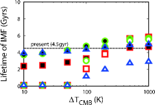
(b)

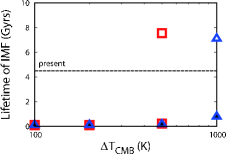
(c)

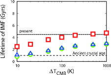
Figure 14: Lifetime of magnetic fields of (a) Mercury, (b) Venus and (c) Mars obtained through our simulations. The free parameters are initial temperature gap at CMB $\Delta T_{\rm CMB}$ and initial impurity concentration in core $x_{0}$, viscosity increase factor $\Delta\eta$, respectively. (a)$\zeta_{m/c}=3:7$, $T_{\rm surf}=440$K, and squares, circles, and triangles are corresponding to models with $x_{0s}=0.01,0.05,$and 0.1, respectively. The filled and open symbols represent models with the standard viscosity and a higher viscosity multiplied by $\Delta\eta=100$. (b)$\zeta_{m/c}=7:3$, $T_{\rm surf}=737$K and $x_{0}=0.1$. The filled and open symbols represent the same meaning as is in the case of Mercury. The square and triangles are models in which one- and two-layered mantle convection are assumed. (c)$\zeta_{m/c}=7:3$, $T_{\rm surf}=210$K. squares, triangles and circles are corresponding to models with $x_{0}=0.1,0.15$ and 0.2.

The lifetime of magnetic fields calculated by our model is shown in Fig. 14. In order to be consistent with current Mercury, Venus and Mars, the lifetime must be longer than 4.5Ga for Mercury and shorter than 4.5Ga for Venus and Mars. Because Martian crust of age $\sim 4$Gyr retains paleomagnetic field, the lifetime of Martian magnetic field may be longer than 0.5 Gyr.

Figures 14 show that for Mercury, the lifetime is longer than 4.5Ga for relatively small values of $x_{\rm 0S}$ ($\sim 0.01-0.05$) except for extremely small $\Delta T_{\rm CMB}$ ($<200-300$K). The relatively long lifetime is resulted by nucleation of inner core due to lower solidification temperature corresponding to small values of $x_{\rm 0S}$. If the nominal value of $x_{\rm 0S}$ is used, the lifetime is short. The small value of $x_{\rm 0S}$ for Mercury was discussed by Stevenson et al. (1983).

The predicted lifetime of magnetic field for Venus is quite short for relatively high mantle viscosity ($\Delta\eta>100$). Observation suggests that Venus is lack of H₂O. That may be due to runaway greenhouse effect of H₂O itself and consequent dissipation by UV dissociation and heating of the molecules. Because melting temperature of the mantle viscosity is lowered by H₂O, relatively high mantle viscosity is more likely, although we do not know exact values of Venus’ mantle viscosity.

The predicted lifetime of magnetic field for for Mars is longer than 1 Gyr but shorter than 4.5Gyr, if initial $\Delta T_{\rm CMB}$ is $\sim 10-500$K. If Mars has never undergone giant impacts that cause significant heating of metallic core, such low initial $\Delta T_{\rm CMB}$ is likely.

Thus, with non-nominal parameters that reflect distance from the Sun and accretion history of individual planets, our model can produce the results that are not inconsistent with the current terrestrial planets in the Solar system. However, in order to clarify intrinsic physics in generation of magnetic field of extra solar terrestrial planets, we focus on the results with the nominal parameters ($T_{\rm surf}=300$K, $\zeta_{\rm m/c}=7:3$, and $x_{\rm 0S}=0.1$), which correspond to the parameters of terrestrial planets with the same compositions as the Earth in habitable zones.

Appendix C. Energy in the core

Figure 15 shows the thermal and gravitational energy, released latent heat, and their sum as a function of $T_{\rm CMB}$ for the nominal cases with planetary mass $M=1,2,5$ and $10M_{\oplus}$, which are calculated by the procedures in section 2.2. We set that each value is zero at the temperature at the initiation of inner core growth. As is shown in this figure, the loss of thermal energy occupies about one third of the total energy loss of the core for the case of $M=1M_{\oplus}$. Released latent heat corresponds to about one fifth of the total energy loss, which depends on $T_{\rm CMB}$ because of the nonlinear density-dependency of the melting temperature of metal.

The gradient of the total energy in Fig. 15 corresponds to an effective specific heat of the core. The total heat capacity is twice larger than the specific heat of thermal energy solely just after the inner core initiation ($T_{\rm CMB}\simeq 4100$K), while their values converge as temperature decreases. This is because impurity concentration increases with the temperature decrease in the outer core. Inner core growth is moderated by the depression of melting temperature of outer core due to the concentration of impurities into outer core. Released gravitational energy and latent heat become smaller than thermal energy as the temperature decreases. Note that the gravitational energy released by the thermal contraction of the core also works as resistance to cooling of the core (see section 2.2).

The ratio of gravitational energy, latent heat and thermal energy is varied with planetary mass. Thermal energy is more dominant than other energies for more massive planet. It means that the gravitational energy and latent heat are not main energy source to drive dynamo action within cores of massive super-Earths. This is mainly because of the change in slope of adiabatic curve within core. The higher gravity causes steeper adiabatic thermal structure, and then core posses large amount of thermal energy inside it for the case of massive planets. This is also the reason why the effective specific heat of core is increased as planetary mass increases.

Table 1: Physical properties of mantle and core components we adopted(Valencia et al., 2007)

material	$\rho_{0}$	$K_{0}$	$K^{\prime}_{0}$	$\gamma_{0}$	$q$	$\theta_{0}$	Refs.
	(kgm-3)	(GPa)
ol	3347	126.8	4.274	0.99	2.1	809	a
wd+rw	3644	174.5	4.274	1.20	2.0	908	a
pv+fmw	4152	223.6	4.274	1.48	1.4	1070	a
ppv+fmw	4270	233.6	4.524	1.68	2.2	1100	b
Fe	8300	164.8	5.33	1.36	0.91	998	c,d
FeS	5330	126	4.8	1.36	0.91	998	c,d

a (Stixrude & Lithgow-Bertelloni, 2005), b (Tsuchiya et al., 2004), c (Williams & Knittle, 1997), d (Uchida et al., 2001)

Table 2: Parameters of radiogenic elements we adopted (van Schmus, 1995)

element	$U$(ppb)	$H$($\mu$Wkg-1)	$\lambda$(yr-1)
K40	28.0	29.17	5.54$\times 10^{-10}$
Th232	76.4	26.38	4.95$\times 10^{-11}$
U235	0.14	568.7	9.85$\times 10^{-10}$
U238	20.1	94.65	1.551$\times 10^{-10}$

Table 3: Parameter of the viscosity in upper mantle and lower mantle (Ranalli, 2001)

	$B$(Pa-ns-1)	n	E∗(103Jmol-1)	V∗(10-6m2mol-1)	$\dot{\epsilon}$(s-1)
upper mantle	3.5$\times 10^{-15}$	3.0	430	10	10-15
lower mantle	7.4$\times 10^{-17}$	3.5	500	10	10-15

Table 4: Physical property of upper mantle, lower mantle, and core (Yukutake, 2000)

	$k_{c}$(W mK-1)	$C_{p}$(J kg-1K-1)	$\alpha$(K-1)
upper mantle	5	1250	3.6$\times 10^{-5}$
lower mantle	10	1260	2.4$\times 10^{-5}$
outer core	40	840	1.4$\times 10^{-5}$

Figure 2: The schematic diagram of the procedure to obtain initial temperature distributions. For more detail, see text.

(a)                                               (b)

(a)                                               (b)

(a)                                               (b)

(a)                                               (b)

(a)

(a)                                               (b)

(a)

(a)                                               (b)

(a)                                               (b)

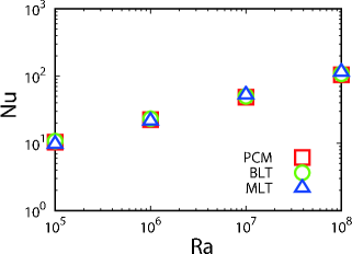
Figure 12: Temporal averaged Nusselt numbers obtained by PCM, BLT and MLT models. Open triangles, circles and squares represent the results of PCM, BLT and MLT models, respectively.

(a)                                       (b)

(a)

$1M_{\oplus}$                                            $2M_{\oplus}$

References

- Abe (1995) Abe, Y. 1995, The Earth’s Central Part: Its Structure and Dynamics, 215
- Abe & Matsui (1985) Abe, Y., & Matsui, T. 1985, in Lunar and Planetary Science Conference Proceedings, Vol. 15, Lunar and Planetary Science Conference Proceedings, ed. G. Ryder & G. Schubert, 545
- Abe & Matsui (1986) Abe, Y., & Matsui, T. 1986, J. Geophys. Res., 91, 291
- Acuña et al. (1999) Acuña, M. H., et al. 1999, Science, 284, 790
- Anderson & Duba (1997) Anderson, O. L., & Duba, A. 1997, J. Geophys. Res., 102, 22659
- Beaulieu et al. (2006) Beaulieu, J., et al. 2006, Nature, 439, 437
- Bullock & Grinspoon (2001) Bullock, M. A., & Grinspoon, D. H. 2001, Icarus, 150, 19
- Canup (2004) Canup, R. M. 2004, Icarus, 168, 433
- Christensen et al. (2009) Christensen, U. R., Holzwarth, V., & Reiners, A. 2009, Nature, 457, 167
- Christensen & Yuen (1985) Christensen, U. R., & Yuen, D. A. 1985, J. Geophys. Res., 90, 10291
- Gaidos et al. (2010) Gaidos, E., Conrad, C. P., Manga, M., & Hernlund, J. 2010, ApJ, 718, 596
- Glatzmaier & Roberts (1995) Glatzmaier, G. A., & Roberts, P. H. 1995, Nature, 377, 203
- Gould et al. (2010) Gould, A., et al. 2010, ArXiv e-prints
- Gubbins et al. (2004) Gubbins, D., Alfè, D., Masters, G., Price, G. D., & Gillan, M. 2004, Geophysical Journal International, 157, 1407
- Gubbins et al. (2003) Gubbins, D., Alfè, D., Masters, G., Price, G. D., & Gillan, M. J. 2003, Geophysical Journal International, 155, 609
- Hale (1987) Hale, C. J. 1987, Nature, 329, 233
- Honda et al. (1993) Honda, S., Yuen, D. A., Balachandar, S., & Reuteler, D. 1993, Science, 259, 1308
- Ida & Lin (2004) Ida, S., & Lin, D. N. C. 2004, ApJ, 604, 388
- Ida & Lin (2008) Ida, S., & Lin, D. N. C. 2008, ApJ, 685, 584
- Ida & Lin (2010) Ida, S., & Lin, D. N. C. 2010, ApJ in press.
- Kageyama & Sato (1997) Kageyama, A., & Sato, T. 1997, Phys. Rev. E, 55, 4617
- Kasting et al. (1993) Kasting, J. F., Whitmire, D. P., & Reynolds, R. T. 1993, Icarus, 101, 108
- Kimura et al. (2009) Kimura, J., Nakagawa, T., & Kurita, K. 2009, Icarus, 202, 216
- Kuang & Bloxham (1997) Kuang, W., & Bloxham, J. 1997, Nature, 389, 371
- Labrosse et al. (2007) Labrosse, S., Hernlund, J. W., & Coltice, N. 2007, Nature, 450, 866
- Léger et al. (2009) Léger, A., et al. 2009, A&A, 506, 287
- Mayor et al. (2009) Mayor, M., et al. 2009, A&A, 493, 639
- Nimmo et al. (2004) Nimmo, F., Price, G. D., Brodholt, J., & Gubbins, D. 2004, Geophysical Journal International, 156, 363
- O’Neill & Lenardic (2007) O’Neill, C., & Lenardic, A. 2007, Geophys. Res. Lett., 34, 19204
- Papuc & Davies (2008) Papuc, A. M., & Davies, G. F. 2008, Icarus, 195, 447
- Queloz et al. (2009) Queloz, D., et al. 2009, A&A, 506, 303
- Ranalli (2001) Ranalli, G. 2001, Journal of Geodynamics, 32, 425
- Sakuraba & Kono (1999) Sakuraba, A., & Kono, M. 1999, Physics of the Earth and Planetary Interiors, 111, 105
- Sasaki & Nakazawa (1986) Sasaki, S., & Nakazawa, K. 1986, J. Geophys. Res., 91, 9231
- Schubert et al. (1979) Schubert, G., Cassen, P., & Young, R. E. 1979, Icarus, 38, 192
- Senshu et al. (2002) Senshu, H., Kuramoto, K., & Matsui, T. 2002, Journal of Geophysical Research (Planets), 107, 5118
- Sharpe & Peltier (1979) Sharpe, H. N., & Peltier, W. R. 1979, Geophysical Journal, 59, 171
- Sohl & Spohn (1997) Sohl, F., & Spohn, T. 1997, J. Geophys. Res., 102, 1613
- Sotin et al. (2007) Sotin, C., Grasset, O., & Mocquet, A. 2007, Icarus, 191, 337
- Spiegel (1963) Spiegel, E. A. 1963, ApJ, 138, 216
- Stevenson et al. (1983) Stevenson, D. J., Spohn, T., & Schubert, G. 1983, Icarus, 54, 466
- Stixrude & Lithgow-Bertelloni (2005) Stixrude, L., & Lithgow-Bertelloni, C. 2005, Geophysical Journal International, 162, 610
- Tajika & Matsui (1992) Tajika, E., & Matsui, T. 1992, Earth and Planetary Science Letters, 113, 251
- Tsuchiya et al. (2004) Tsuchiya, T., Tsuchiya, J., Umemoto, K., & Wentzcovitch, R. M. 2004, Earth and Planetary Science Letters, 224, 241
- Uchida et al. (2001) Uchida, T., Wang, Y., Rivers, M., & Sutton, S. 2001, J. Geophys. Res, 106, 21799
- Udry et al. (2007) Udry, S., et al. 2007, A&A, 469, L43
- Umemoto et al. (2006) Umemoto, K., Wentzcovitch, R. M., & Allen, P. B. 2006, Science, 311, 983
- Usselman (1975) Usselman, T. 1975, American Journal of Science, 275, 278
- Valencia et al. (2006) Valencia, D., O’Connell, R. J., & Sasselov, D. D. 2006, Icarus, 181, 545
- Valencia et al. (2007) Valencia, D., O’Connell, R. J., & Sasselov, D. D. 2007, ApJ, 670, L45
- Valencia et al. (2007) Valencia, D., Sasselov, D. D., & O’Connell, R. J. 2007, ApJ, 656, 545
- van Schmus (1995) van Schmus, W. R. 1995, Global Earth Physics, A Handbook of Physical Constants, AGU Reference Shelf, 1, 283
- Vinet et al. (1987) Vinet, P., Ferrante, J., Rose, J., & Smith, J. 1987, Journal of Geophysical Research-Solid Earth, 92
- Vitense (1963) Vitense, E. 1963, Zs. f. Ap., 32, 135
- Williams & Knittle (1997) Williams, Q., & Knittle, E. 1997, Physics of the Earth and Planetary Interiors, 100, 49
- Wortel & Spakman (2000) Wortel, M. J. R., & Spakman, W. 2000, Science, 290, 1910
- Yukutake (2000) Yukutake, T. 2000, Physics of the Earth and Planetary Interiors, 121, 103
- Zahnle et al. (1988) Zahnle, K. J., Kasting, J. F., & Pollack, J. B. 1988, Icarus, 74, 62