Modelling of the Complex CASSOWARY/SLUGS Gravitational Lenses

Abstract

We present the first high-resolution images of CSWA 31, a gravitational lens system observed as part of the SLUGS (Sloan Lenses Unravelled by Gemini Studies) program. These systems exhibit complex image structure with the potential to strongly constrain the mass distribution of the massive lens galaxies, as well as the complex morphology of the sources. In this paper, we describe the strategy used to reconstruct the unlensed source profile and the lens galaxy mass profiles. We introduce a prior distribution over multi-wavelength sources that is realistic as a representation of our knowledge about the surface brightness profiles of galaxies and groups of galaxies. To carry out the inference computationally, we use Diffusive Nested Sampling, an efficient variant of Nested Sampling that uses Markov Chain Monte Carlo (MCMC) to sample the complex posterior distributions and compute the normalising constant. We demonstrate the efficacy of this approach with the reconstruction of the group-group gravitational lens system CSWA 31, finding the source to be composed of five merging spiral galaxies magnified by a factor of 13.

1 Introduction

Gravitational lensing has revealed itself to be a powerful probe of not only the distribution of luminous and dark matter within the lensing galaxies, but also the small scale structure apparent in sources when the images are reconstructed. Initially, with point-like quasar sources, only limited information was available to constrain reconstructions, but the identification of extended images has led to the development of a number of techniques to maximize the use of additional information in determining both the lens and source properties (for a recent review of strong lensing by galaxies, see Treu, 2010).

The development of large scale surveys has allowed for the automatic search and identification of large numbers of gravitational lens systems. A prominent example is SLACS (Sloan Lens ACS Survey), which uses HST/ACS to follow-up lens candidates identified in the Sloan Digital Sky Survey (SDSS) (Bolton et al., 2008). SLACS targets small separation lenses, in which the images are unresolved by SDSS, typically through the spectroscopic identification of emission lines from high redshift objects within the spectra of lower redshift early-type galaxies. Thus, SLACS has been highly successful in using lensing to study the properties of typical elliptical galaxies (Treu et al., 2009).

Alternatively, the Cambridge And Sloan Surey of Wide ARcs in the skY (CASSOWARY) survey (Belokurov et al., 2009, http://www.ast.cam.ac.uk/research/cassowary/), explores a different regime of galaxy-galaxy lens systems by searching for multiple blue faint companions around massive luminous red galaxies in SDSS. Thus, CASSOWARY is suited to finding wide separation lenses with high magnification. So far, CASSOWARY has identified 40 systems, with several more unconfirmed candidates. These lenses are suited to utilising the unique properties of gravitational lensing to provide information about the mass profiles of massive galaxies and galaxy groups, and to provide very high resolution images of faint high-redshift galaxies. Previous studies of group lenses include Limousin et al. (2009).

In this paper we present the first analysis of high resolution Gemini/GMOS images of a confirmed CASSOWARY lens system, taken as part of the SLUGS (Sloan Lenses Unraveled by Gemini Studies) program. The focus of this paper is the reconstruction technique, with the details of the extension to other CASSOWARY lenses being presented elsewhere (Belokurov et al in prep.) In Section 2, we describe the approach to gravitational lens modelling that will be adopted for the SLUGS systems, discussing the prior source information in Section 2.1, the adopted lens models in Section 2.2, and the implementation of nested sampling in Section 4. The second part of the paper, Section 5, we will present the implementation of this scheme on CSWA 31; a newly confirmed gravitational lens and part of the SLUGS sample. The conclusions of this study are presented in Section 6.

2 Gravitational Lens Reconstruction

Gravitational lens reconstruction is a classic inference problem (Brewer & Lewis, 2006): given some data $D$ (i.e. image pixel values) and prior information (and/or assumptions), we wish to infer various properties of the lens system such as its source parameters $S$, the lens parameters $L$, and various other parameters, denoted collectively by $\Phi$; for example, $\Phi$ may include parameters describing the light profile of the lens galaxy, and unknown noise levels or systematic effects. By Bayes’ rule, our knowledge of these parameters, taking into account the data, is described by the posterior probability distribution

$$p(S,L,\Phi|D)\propto p(S,L,\Phi)p(D|S,L,\Phi)$$ (1)

$$=p(S)p(L|S)p(\Phi|L,S)p(D|S,L,\Phi)$$ (2)

Different lens modelling techniques can all be interpreted within this framework (Brewer & Lewis, 2006). Differences between them are mostly due to the effective choices for the probability distributions $p(S,L,\Phi)$, describing prior knowledge about the system, and $p(D|S,L,\Phi)$, describing prior knowledge about how the observed data are related to the system. The other area where lens modelling techniques differ is the strategy for summarising the posterior distribution: typically one either searches for the peak to find a best-fitting model, or else one tries to obtain a sample of typical models from the posterior distribution. The latter approach is more computationally expensive but results in a more honest summary of the uncertainty in the conclusions, as the posterior probability of any hypothesis can be easily calculated. Throughout this paper, we will use a sampling-based approach, prioritising realism over convenience.

2.1 A Realistic Prior on Sources

To begin the inference, we must construct a prior probability distribution to describe what kinds of sources are considered plausible. Ideally, the prior distribution should contain all of the relevant information that we have about typical light profiles of galaxies, but should otherwise make minimal assumptions about features of the light profile that we are actually uncertain about. We will now list features that an ideal prior distribution for a galaxy source should have. Various priors have been proposed and used in the literature, usually satisfying some of these criteria but not others. In Section 2.1.1 we develop a prior that has all of these properties. This is not to claim that our prior is optimal, or the best one could do, merely that it avoids some of the most obvious flaws.

• The surface brightness should be non-negative everywhere, with 100% prior probability. This rules out the use of “linear regularisation”, i.e. pixellated intensity maps with a joint Gaussian prior for the intensity values (e.g. Suyu et al., 2006; Dye et al., 2008).
  

• The surface brightness may be close to zero over a large fraction of the domain (Brewer & Lewis, 2006). This rules out pixellated intensity maps with constrained uniform prior, and the “maximum entropy” prior (Wallington, Kochanek, & Narayan, 1996).
  

• Surface brightness at one point should be correlated with surface brightness at another nearby point. This correlation should decrease with distance.
  

• The degree of spatial correlation may vary across the domain: i.e. we should not rule out the possibility of smoothness in one region and small scale structure in another.
  

• The prior should be convenient to explore via Markov Chain Monte Carlo (MCMC).
  

• There is probably some degree of correlation between the surface brightness profile in different wavebands, although this is not guaranteed.

The statistics literature contains many proposals for general prior distributions for density functions (e. g. the Dirichlet distribution), which may be adapted for our purpose; however, the context here is different: our densities will be surface brightness profiles and not probability densities for data points. Thus, our concern is not so much with the mathematical properties of the priors but with which ones produce density profiles that resemble galaxies. We attempt to satisfy all of the design criteria listed above with our blobby prior described in the next section.

2.1.1 Blobby Prior

Our models of surface brightness profiles will ultimately be constructed from some basis functions, also known colloquially as “blobs”. Specifically, we choose elliptical Sérsic profiles as our basis functions, since in some cases even a single Sérsic profile is sufficient to describe the light profile of a galaxy. This approach of using moderate numbers of physically motivated profiles is not new (e.g. Marshall, 2006; Skilling, 1998), but is a simple way of implementing a prior with the desired properties outlined above.

In a suitably centred and aligned Cartesian coordinate system, a blob with scale radius $R_{0}$ and axis ratio $q$ has the following profile:

$$f(x,y)=C\exp\left[-\left(\frac{R}{R_{0}}\right)^{\alpha}\right]$$ (3)

where $R=\sqrt{x^{2}/q+qy^{2}}$. When $\alpha=2$, the blob is a Gaussian; $\alpha=1$ corresponds to an exponential profile, and $\alpha=1/4$ is the de Vaucouleurs profile. We restrict $\alpha$ to be between 0.1 and 10. We also allow the number of blobs, numBlobs, to be a free parameter.

Since we will be analysing multi-band images, we must also assign a prior probability distribution to the colours of the blobs. To accomplish this, each blob has a set of parameters called unnormalisedSpectrum, describing how bright the blob is in each band relative to the other bands. The blobs can all have similar colours, or the colours can vary immensely. The degree of diversity of the spectra is controlled by a hyperparameter called sigSpectrum. The hyperparameter meanSpectrum describes the typical colour that the blobs are centred around.

The prior for the central positions of the blobs was chosen to be a an independent Gaussian distribution for each blob, with a common centre position and standard deviation, as hyperparameters. This allows the blobs to be either close to concentric, or not, as required by the data. If the blobs are almost concentric, then sums of several blobs can accurately model most decreasing radial profiles. Multi-component sources can also be modelled, they correspond to the case where the blobs are separated by more than about one scale radius. We have experimented with more sophisticated schemes to correlate the central positions of the blobs (Neal, 2003) but found that the gain in realism was minor, yet the computational complexity of the problem increased significantly.

The typical peak surface brightness of blobs was assigned a prior that spans several orders of magnitude, centred around unity. Thus, the reconstruction software expects images in units where the fluxes are of order close to unity. The actual peak surface brightness of each blob has a lognormal prior, centered around the typical value.

For a thorough description of all of the parameters and the prior distributions that define our blobby prior, see Table 1. Figure 1 shows sample galaxy light profiles drawn from the prior. We recommend, as a general practice, generating random models from the prior as a visual check on the reasonableness of the prior probability assignments.

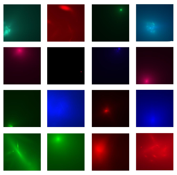
Figure 1: A sample of random light profiles (source galaxies generated from the prior distribution defined in Section 2.1.1. Simple and complex profiles are possible, as are a variety of sizes and colours. The peak surface brightness is also uncertain by several orders of magnitude. While this prior clearly is not an optimal assignment, it is a more realistic assignment than regularisation formulae (Suyu et al., 2006), for which the corresponding images would resemble noise (for first-order regularisation) or blurred noise (for gradient or curvature regularisation).

Table 1: All of the parameters of a multi-wavelength blobby light profile, and their prior distributions. If the prior for a parameter refers to a hyperparameter, then this defines the prior conditional on that hyperparameter. The priors for the hyperparameters themselves are included in the second half of the table. All priors are independent except where otherwise specified. $J(a,b)$ denotes Jeffreys’ scale-invariant prior $p(x)\propto 1/x$ between lower and upper bounds of $a$ and $b$ respectively. Lognormal$(a,b^{2})$ denotes a lognormal distribution, with $a$ being the central value for the variable, and $b$ being the standard deviation for the log of the variable. Note that $a$ may be named $\texttt{mean}*$, even though it is not technically the mean of the distribution.

Parameter	Definition	Prior
Individual Blob Parameters
peak	Peak surface brightness, $C$ in Eqn 3	Lognormal(meanPeak, stdevLogPeak2)
width	Scale width ($R_{0}$ in Eqn 3)	Exponential(meanWidth)
xc, yc	Central position	Normal(($X_{c},Y_{c}$), $\texttt{spread}^{2}$)
q	Axis ratio	Uniform(0.1,1)
theta	angle of Orientation	Uniform$(0,2\pi)$
slope	Slope of light profile, $\alpha$ in Eqn 3	Lognormal($\texttt{meanAlpha},\texttt{sigAlpha}^{2}$)
unnormalisedSpectrum	Share of bolometric flux at each wavelength	Lognormal$(\texttt{meanSpectrum},\texttt{sigSpectrum}^{2})$
Hyperparameters
numBlobs	Number of blobs	Uniform($\left\{0,1,2,...,10\right\}$)
$(X_{c},Y_{c})$	Typical position that blobs are centred around	Uniform over source domain
spread	Standard deviation of blob positions	$J(10^{-3},1)\times$ (image width)
meanPeak	Typical brightness of a blob	$J(10^{-3},10^{3})$
stdevLogPeak	Diversity of brightness of blobs	$J(0.03,2)$
sigSpectrum	Diversity of spectra	$J(0.01,3)$
meanWidth	Typical scale width of a blob	$J(10^{-3},1)\times$ (image width)
meanSpectrum	Typical spectrum that blob spectra are centred around	Lognormal(0, $3^{2}$)
meanAlpha	Typical slope	$J(0.1,10)$
sigAlpha	Diversity of slopes	$J(0.01,2)$

2.2 Lens Models

In cases where the light profile of the lens galaxy appears simple, we assume that the mass profile is also simple and model the projected mass profile of the lens galaxy as a nonsingular isothermal ellipsoid (NIE) plus external shear ($\gamma$). This model (and related models, e.g. singular isothermal ellipsoid without external shear) has been used very successfully to model the mass profiles of elliptical galaxy lenses (e.g. Bolton et al., 2008); even when more general models have been used, the mass profiles are inferred to be close to isothermal. The model has eight parameters: $b$, the “Einstein radius”, $q$, the axis ratio of the major and minor axes of the elliptical mass distribution, $(x_{c},y_{c})$, the central position of the lens, $\theta$, the orientation angle of the lens, $\gamma$, the strength of the external shear, $\theta_{\gamma}$, the orientation angle of the external shear, and $r_{c}$, the core radius (often set to zero, giving a singular isothermal ellipsoid). A simple interpretation of $b$ is the length of the minor axis of the critical curve, in the singular case $r_{c}=0$.

The source plane position $(x_{s},y_{s})$ and the image plane position $(x,y)$ of a ray are related by:

$$x_{s}=x-\alpha_{x}(x,y)$$

$$y_{s}=y-\alpha_{y}(x,y)$$ (4)

where the deflection angles $\alpha$ are given by Keeton & Kochanek (1998). Defining $\psi=\sqrt{q^{2}(r_{c}^{2}+x^{2})+y^{2}}$, the deflection angle formulae are:

$$\alpha_{x}(x,y) = \frac{b}{\sqrt{1-q^{2}}}\tan^{-1}\left[\frac{x\sqrt{1-q^{2}}}{\psi+r_{c}}\right]$$ (5)

$$\alpha_{y}(x,y) = \frac{b}{\sqrt{1-q^{2}}}\tanh^{-1}\left[\frac{y\sqrt{1-q^{2}}}{\psi+q^{2}r_{c}}\right]$$ (6)

as long as $q<1$. If $q>1$, then $q$ can simply be replaced by $q^{-1}$ and the orientation angle $\theta$ rotated by 90 degrees, with the same result. We do not allow $q=1$ but it can become arbitrarily close to 1 and therefore close-to-spherical lenses are not ruled out. By making the prior for the lens strength $b$ depend on the image size, we are able to avoid the need for system-specific tuning of the priors: we simply assume that the input images are such that the Einstein Radius $b$ of the lens is of the same scale as the input image.

2.3 Complex Lenses

Since the SLUGS sample contains very massive lenses, many of the lenses are not smooth galaxies but are instead galaxy groups. For modelling these systems, the NIE family is not flexible enough to represent the complex structure of the lens. To overcome this, it is possible to use the blobby prior of Section 2.1.1, but interpret each blob as a nonsingular isothermal ellipsoid (with zero external shear) rather than a Sérsic profile. This is straightforward as there is a simple correspondence between the parameters of the Sérsic profile and the parameters of the NIE. However, this creates computational inefficiencies, as the code needs to infer the positions and orientations of many lens components, and the likelihood function tends to be more difficult when modifying the lens as opposed to the source. We note that gravitational interactions within groups will tend to make the NIE approximation for each galaxy less valid, however sums of NIEs remain a tractable and flexible family of models.

For complex lenses in the SLUGS sample, we use the following strategy. First, we visually identify the approximate positions, ellipticities and orientations of the dominant lens components. The prior for these parameters can then be set to be narrow Gaussians centred on the estimated values. The Einstein radii $\{b\}$ of these lenses can then be assigned a broad prior, such as independent $\propto 1/b$ priors within a generous range. This prior suggests that from the images, we know where the lens substructures are, but we do not know their relative masses, because the mass to light ratio might differ between objects.

3 Sampling Distributions

The prior distributions for the unknown parameters have now all been defined. However, we must also assign sampling distributions $p(S,L,\Phi|D)$ for all $D$ and $(S,L,\Phi)$ (these are known as sampling distributions when $D$ is unknown, when $D$ is fixed at the observed data, $p(S,L,\Phi|D)$ as a function of the parameters is called the likelihood function). For any value of the source and lens parameters $(S,L)$ we can compute mock images $M(S,L)$ by ray tracing through the lens (firing 4 rays per image pixel, a compromise value chosen for efficiency) and blurring by the PSF (assumed known from nearby stars in the field). The likelihood is then related to the $\chi^{2}$ deviation between the mock image and the actual image; i.e. we assume a sampling distribution for the noise that is normal/Gaussian with mean 0, and independent for each pixel:

$$p(D|S,L,\Phi)=$$

$$\exp\left[-\frac{1}{2}\sum_{i=1}^{n}\left\{\log(2\pi\sigma_{i}^{2})+\left(\frac{D_{i}-M(S,L)_{i}}{\sigma_{i}}\right)^{2}\right\}\right]$$ (7)

where $n$ is the total number of pixels, and the standard deviation for each pixel is given by:

$$\sigma_{i}=\sqrt{\sigma_{{\rm map},i}^{2}+\sigma_{{\rm base}}^{2}+\left(\tau\sqrt{M(S,L)_{i}}\right)^{2}}$$ (8)

Here, $\sigma_{{\rm map}}$ is the uncertainty reported from the weight map, and the extra parameters $\sigma_{{\rm base}}$ and $\tau$ allow for inaccuracies in the weight map, by possibly boosting the noise level by a constant value, or a value proportional to the square root of the predicted surface brightness. $\sigma_{{\rm base}}$ and $\tau$ were assigned $J(10^{-3},10^{3})$ priors. Once again, this assumes that the input images are in units where the typical pixel values are of order unity.

Although it is not presented in this paper, we also recommend generating simulated data sets from the sampling distribution, using models drawn from the prior. This practice gives visual checks on the joint prior, $p(\theta,D)=p(\theta)p(D|\theta)$ which inference depends on.

The computational task of using images to infer appropriate values for all of the above parameters, with uncertainties, is rather difficult. To accomplish this goal, we use a variant of Nested Sampling (Skilling, 2006), designed to cope effectively with multimodal and highly correlated posterior distributions. This algorithm is described briefly in Section 4. For a full description, see Brewer, Pártay, & Csányi (2010).

4 Nested Sampling Implementation

Nested Sampling (NS) is a powerful and widely applicable algorithm for Bayesian computation (Skilling, 2006). Starting with a population of particles $\{\theta_{i}\}$ drawn from the prior distribution $\pi(\theta)$, the worst particle (lowest likelihood $L(\theta)$) is recorded and then replaced with a new sample from the prior distribution, subject to the constraint that its likelihood must be higher than that of the point it is replacing. As this process is repeated, the population of points moves progressively higher in likelihood.

Each time the worst particle is recorded, it is assigned a value $X\in[0,1]$, which represents the amount of prior mass estimated to lie at a higher likelihood than that of the discarded point. Assigning $X$-values to points creates a mapping from the parameter space to $[0,1]$, where the prior becomes a uniform distribution over $[0,1]$ and the likelihood function is a decreasing function of $X$. Then, the evidence can be computed by simple numerical integration, and posterior weights can be assigned by assigning a width to each point, such that the posterior mass associated with the point is proportional to width $\times$ likelihood.

The key challenge in implementing Nested Sampling for real problems is to be able to generate the new particle from the prior, subject to the hard likelihood constraint. If the discarded point has likelihood $L^{*}$, the newly generated point should be sampled from the constrained distribution:

$$p_{L^{*}}(\theta)=\frac{\pi(\theta)}{X^{*}}\left\{\begin{array}[]{lr}1,&L(\theta)>L^{*}\\ 0,&\textnormal{otherwise.}\end{array}\right.$$ (9)

where $X^{*}$ is the normalising constant. Technically, our knowledge of this new point should be independent of all of the surviving points. A simple way to generate such a point is suggested by Sivia & Skilling (2006): copy one of the surviving points and evolve it via MCMC with respect to the prior distribution, rejecting proposals that would take the likelihood below the current cutoff value $L^{*}$. This evolves the particle with Equation 9 as the target distribution. If the MCMC is done for long enough, the new point will be effectively independent of the surviving population and will be distributed according to Equation 9. However, in complex problems, this approach can easily fail - constrained distributions can often be very difficult to efficiently explore via MCMC, particularly if the posterior distribution is multimodal or highly correlated. To overcome these drawbacks, sophisticated schemes such as MultiNest (Feroz, Hobson, & Bridges, 2008) have been developed and applied successfully in low-dimensional problems. However, for our purposes we require a method that uses MCMC.

The main advantage of Nested Sampling is that successive constrained distributions (i.e. $p_{L^{*}_{j}}(\theta),p_{L^{*}_{j+1}}(\theta)$, and so on) are, by construction, all compressed by the same factor relative to their predecessor. This is not the case with tempered distributions of the form $p_{T}(\theta)\propto\pi(\theta)L(\theta)^{1/T}$, where a small change in temperature $T$ can correspond to a small or a large compression. Tempering based algorithms (e.g. simulated annealing, parallel tempering) will fail unless the density of temperature levels is adjusted according to the specific heat, which becomes difficult at a first-order phase transition. Unfortunately, knowing the appropriate values for the temperature levels is equivalent to having already solved the problem! Nested Sampling does not suffer from this issue because it asks the question “what should the next distribution be, such that it will be compressed by the desired factor”, rather than the tempering question “the next distribution is pre-defined, how compressed is it relative to the current distribution?”

4.1 Diffusive Nested Sampling

Throughout this paper we use the efficient Diffusive Nested Sampling method (Brewer, Pártay, & Csányi, 2010) which has been found to speed up MCMC-based Nested Sampling by an order of magnitude. The basic idea is that, instead of exploring a single constrained distribution, the particle explores a mixture of the required constrained distribution, and the past constrained distributions (See Figure 2). New likelihood contours are created using likelihoods accumulated during the run, which provides more information than using only the likelihood value of the endpoint of an MCMC run. Finally, the absence of the copying operation prevents the depletion problem that can occur in the classic implementation of NS, where repeated copying destroys the diversity of the population of particles prematurely. For more details, see Brewer, Pártay, & Csányi (2010).

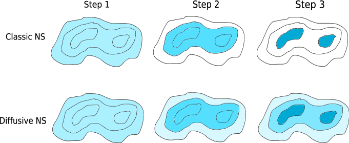
Figure 2: An illustration of a the distributions that must be sampled as Nested Sampling progresses (Brewer, Pártay, & Csányi, 2010). In the classic scheme, at Step 3, we must obtain a sample from the coloured region which is composed of two separate islands, which is usually very difficult if MCMC is the only exploration option. To overcome these difficulties, we explore the mixture distribution (bottom right), where travel between isolated modes is more likely.

4.2 Nested Sampling Solves Multiple Problems at Once

Nested Sampling algorithms provide samples from the parameter space, along with an assignment of prior mass (width in the $X$-space) to each sample. These samples can be used to probe (generate samples and estimate the normalising constant) target probability distributions other than the posterior. For example, a common family of distributions of interest are the tempered posterior distributions:

$$p_{T}(\theta)=\frac{1}{Z(T)}\pi(\theta)L(\theta)^{1/T}$$ (10)

These distributions can be studied by weighting the particles according to $\left(\texttt{prior mass}\right)$ $\times L^{1/T}$, for various $T$ rather than just $T=1$.

Of course, this is only possible if the sample contains points from regions of parameter space that are significant with respect to the modified target distribution.

This technique can be used to solve the inference problem under different prior probability assignments at very little computational cost. Particularly, we can explore the effect of different sampling distributions (Section 3). For example, suppose we hypothesise a correlated probability distribution for the noise. This means that larger, correlated deviations between the model and the data can be ascribed to noise, rather than model inadequacy. Thus, samples with lower $X$-values will be deemed acceptable and included in the sample. The effect of correlated noise models is very similar to the effect of simply raising the temperature, an operation that is computationally trivial.

Note that not all systematic errors can be accounted for in this way. For example, imagine that the sky background had been subtracted incorrectly, leaving a gradient across the image. This would be modelled using light in the source plane. If we attempted to reweight the sample by using the marginal likelihood after integrating over a prior distribution for the incorrect sky subtraction, we would find that one point dominated the sample. This immediately provides evidence of failure: essentially, Nested Sampling would have scaled the wrong peak in parameter space, and did not obtain any significant samples with respect to the modified posterior. This situation is easily identified (only a single particle will have significant weight) and is analogous to using a poor approximating distribution in standard importance sampling.

5 CSWA 31

CSWA 31 is a complex lens with at least seven identifiable images and a very large image separation ($\sim$ 12”)(Figure 3). The lens is a galaxy group, with a dominant central galaxy acting as the primary lens. We obtained g,r, and i-band images for CSWA31 on February 21, 2009, using the GMOS instrument on the Gemini South telescope. 1200 second dithered exposures were obtained in each of the bands, in seeing ranging from 0.7-0.75”. The GMOS field of view is 5.5 x 5.5 arcmin, and with 2x2 binning, the image scale is 0.145”/pixel. In Figures 3-5, north is towards the bottom of the page.

Due to the presence of mass substructure (as seen by the large number of yellow blobs in the image), we used the complex lens model (Section 2.3) for this system. The dominant yellow sources in the image were modelled as 11 SIE lenses, with their positions, ellipticities and orientation angles almost-fixed at the observed values from the light (the prior allowed for a small uncertainty in each). We allowed the Einstein radii $\{b\}$ to be free parameters with independent scale-free priors, truncated such that the primary lens must have the highest $b$. The central positions of the lens blobs are shown in Figure 4.

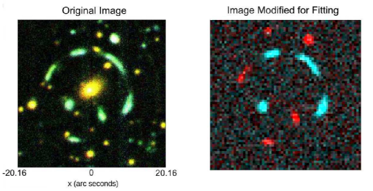
Figure 3: SLUGS Gemini/GMOS Image of CSWA 31, with the primary lens galaxy subtracted (left). The right hand image shows the bluest image of CSWA 31 (where the redder lens substructures are not visible), resampled onto a 64$\times$64 pixel grid, for computational speed. Only the brightest lensed images were retained. Preliminary studies indicated that four of the images (the blue images in the modified image) are a classic quad configuration. For computational reasons we gave these images a common colour, to help our algorithm find the correct model more quickly.

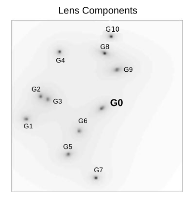
Figure 4: Mean positions of the SIE lenses for the complex lens model for CSWA 31. The prior uncertainty on the positions is 1”. The relative masses are left as free parameters, with broad priors. The eleven lens components chosen were the ones that appear most luminous and close to images, and therefore most likely to be significant lenses. Not all of the yellow components in Figure 3 were included for computational efficiency.

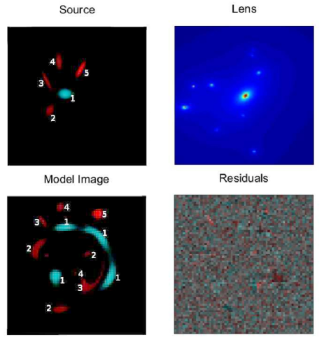
Figure 5: A typical model from the posterior distribution for the CSWA 31 reconstruction. The source is composed of five components, separated on the sky by $\sim$ 3 arcseconds. The primary source (1) is lensed into a classic quad configuration. (2) has been lensed in a complex manner into three main images, and (3) is doubly imaged,

Unfortunately the complex lens model creates large computational overheads: the time taken to simulate an image increases with the number of lens “blobs”. Additional computational expense is caused by the fact that the parameter space now has more dimensions, causing Diffusive Nested Sampling to require more steps per new level, and more levels to reach the bulk of the posterior. Finally, the large separation of the lens implies that the image simply has more pixels. To reduce the effect of these computational challenges, we analyse only a degraded resolution version of the CSWA 31 image, containing only the most significant images (Figure 3 shows the full and the degraded image). This means our final reconstruction will have only the brightest of the source components that are actually present.

A further challenge is caused by the fact that it is not clear which sources are in the lens plane and which are background sources, and even whether the background sources are all at the same redshift. For this initial study, we assume that all images in the right panel of Figure 3 are images of sources lying at a single redshift.

The modelling was run with a maximum of five sources. A typical model from the run is shown in Figure 5. The source is comprised of five galaxies of extent $\sim 2^{\prime\prime}$, separated by $\sim 5^{\prime\prime}$. The source (1) has been lensed into a classic quad configuration by the primary lens. Note that, according to our model, the leftmost image of (2) and the rightmost image of (3) are different sources and so may be different colours, whereas they appear to match in the image (Figure 3). We attempted to find models where these two images are images of the same source, but we were unable to do so. The image in Figure 3 shows additional small green sources that may also lie scattered throughout the source group.

Unfortunately the source redshifts are unknown so the physical scale is also unknown, however we are able to provide an estimate. The redshift of the lens is 0.683. Assuming a source redshift $z_{s}=1$ gives a source plane scale of 8.3 kpc$/^{\prime\prime}$, implying that these source galaxies are large spirals. Assuming $z_{s}=0.8$ gives 7.7 kpc$/^{\prime\prime}$ and $z_{s}=2$ gives 9.3 kpc$/^{\prime\prime}$, so the physical interpretation is insensitive to the source redshift. The magnification of the source is $2.8\pm 0.1$ magnitudes, a factor of $\sim 14$.

We measure the mass of the primary lens, within its critical curve, to be $1.4\pm 0.2\times 10^{13}M_{\odot}$. The other lenses masses are significantly uncertain, so we do not report them here.

6 Conclusions

In this paper we have detailed the lens modelling technique to be used for the complex gravitational lenses in the SLUGS (Sloan Lenses Unravelled by Gemini Studies) sample. The main features of our technique are the attempt to incorporate realistic prior information about galaxy surface brightness profiles, and the Diffusive Nested Sampling method for exploring the posterior distribution for the reconstructions. We recommend drawing random samples from complex prior distributions as a visual check on the reasonableness of the probability assignments. Our random samples qualitatively resemble simple galaxy profiles, whereas the corresponding random samples from other methods, such as linear regularisation, are simply noise. Hence, our method uses much more prior information and can be expected to perform better than the alternatives when the data are noisy or low resolution.

We presented the first reconstruction of the complex SLUGS lens CSWA 31. We found that the observed lensing configuration is best explained by five source components, lensed into the elaborate image structure by the complex group lens. Although the source redshift is unknown, it is plausible that the physical sizes of the sources are $\sim 10$ kpc and hence we are observing the merger of five large spiral galaxies.

7 Acknowledgements

BJB is grateful to Lianne Zimmermann for helping him to settle in to Santa Barbara. I would also like to thank Matt Auger and Phil Marshall for advice about modelling CSWA 31, and Tommaso Treu for valuable comments.

References

- Belokurov et al. (2007) Belokurov V., et al., 2007, ApJ, 671, L9
- Belokurov et al. (2009) Belokurov V., Evans N. W., Hewett P. C., Moiseev A., McMahon R. G., Sanchez S. F., King L. J., 2009, MNRAS, 392, 104
- Bolton et al. (2008) Bolton A. S., Burles S., Koopmans L. V. E., Treu T., Gavazzi R., Moustakas L. A., Wayth R., Schlegel D. J., 2008, ApJ, 682, 964
- Brewer, Pártay, & Csányi (2010) Brewer B. J., Pártay L. B., Csányi G., 2010, “Diffusive Nested Sampling”, Statistics and Computing, DOI: 10.1007/s11222-010-9198-8. arXiv:0912.2380
- Brewer & Lewis (2006) Brewer B. J., Lewis G. F., 2006, ApJ, 637, 608
- Brewer & Lewis (2006) Brewer B. J., Lewis G. F., 2006, ApJ, 651, 8
- Dye et al. (2008) Dye S., Evans N. W., Belokurov V., Warren S. J., Hewett P., 2008, MNRAS, 388, 384
- Feroz, Hobson, & Bridges (2008) Feroz F., Hobson M. P., Bridges M., 2008, arXiv, arXiv:0809.3437
- Keeton & Kochanek (1998) Keeton C. R., Kochanek C. S., 1998, ApJ, 495, 157
- Limousin et al. (2009) Limousin M., et al., 2009, A&A, 502, 445
- Maller et al. (2000) Maller A. H., Simard L., Guhathakurta P., Hjorth J., Jaunsen A. O., Flores R. A., Primack J. R., 2000, ApJ, 533, 194
- Marshall (2006) Marshall P., 2006, MNRAS, 372, 1289
- Neal (2003) Neal, R. M., 2003, “Density modeling and clustering using Dirichlet diffusion trees”, Bayesian Statistics 7, pp. 619-629
- Pártay, Bartók, & Csányi (2009) Pártay L. B., Bartók A. P., Csányi G., 2009, arXiv, arXiv:0906.3544
- Quider et al. (2009) Quider A. M., Pettini M., Shapley A. E., Steidel C. C., 2009, MNRAS, 398, 1263
- Sivia & Skilling (2006) Sivia, D. S., Skilling, J., 2006, Data Analysis: A Bayesian Tutorial, 2nd Edition, Oxford University Press
- Skilling (1998) Skilling J., 1998, Massive Inference and Maximum Entropy, in Maximum Entropy and Bayesian Methods, Kluwer Academic Publishers, Dordrecht/Boston/London p.14
- Skilling (2006) Skilling, J., 2006, “Nested Sampling for General Bayesian Computation”, Bayesian Analysis 4, pp. 833-860
- Suyu et al. (2006) Suyu S. H., Marshall P. J., Hobson M. P., Blandford R. D., 2006, MNRAS, 371, 983
- Treu (2010) Treu T., 2010, ARA&A, 48, 87
- Treu et al. (2009) Treu T., Gavazzi R., Gorecki A., Marshall P. J., Koopmans L. V. E., Bolton A. S., Moustakas L. A., Burles S., 2009, ApJ, 690, 670
- Wallington, Kochanek, & Narayan (1996) Wallington S., Kochanek C. S., Narayan R., 1996, ApJ, 465, 64