Analysis and Design of Tuned Turbo Codes

Abstract

It has been widely observed that there exists a fundamental trade-off between the minimum (Hamming) distance properties and the iterative decoding convergence behavior of turbo-like codes. While capacity achieving code ensembles typically are asymptotically bad in the sense that their minimum distance does not grow linearly with block length, and they therefore exhibit an error floor at moderate-to-high signal to noise ratios, asymptotically good codes usually converge further away from channel capacity. In this paper, we introduce the concept of tuned turbo codes, a family of asymptotically good hybrid concatenated code ensembles, where asymptotic minimum distance growth rates, convergence thresholds, and code rates can be traded-off using two tuning parameters, $\lambda$ and $\mu$. By decreasing $\lambda$, the asymptotic minimum distance growth rate is reduced in exchange for improved iterative decoding convergence behavior, while increasing $\lambda$ raises the asymptotic minimum distance growth rate at the expense of worse convergence behavior, and thus the code performance can be tuned to fit the desired application. By decreasing $\mu$, a similar tuning behavior can be achieved for higher rate code ensembles.

I Introduction

Turbo codes [1] and multiple parallel concatenated codes (MPCCs) [2] perform very close to the Shannon limit with suboptimum iterative decoding, but the corresponding code ensembles are asymptotically bad in the sense that their minimum (Hamming) distance does not grow linearly with block length [3]. Even the minimum distance of the best code in the ensemble of turbo codes cannot grow more than logarithmically with block length [4]. As a result, their minimum distance may not be sufficient to yield very low error rates at moderate-to-high signal to noise ratios (SNRs), and an error floor can occur.

On the other hand, multiple serially concatenated code (MSCC) ensembles with three or more component encoders can be asymptotically good. This has been shown for repeat multiple accumulate codes in [5, 6, 7]. There also exist variations of standard repeat accumulate codes that are asymptotically good [8] but are more complex to encode than classical repeat accumulate codes.

MSCCs in general exhibit good error floor performance due to their large minimum distance, but they have the drawback of converging at an SNR further from capacity than parallel concatenated codes. While the asymptotic distance growth rate of MSCCs can be made arbitrarily close to the Gilbert-Varshamov Bound (GVB) by adding more concatenation stages [7], the iterative decoding convergence behavior of the resulting code ensembles becomes worse, making codes with more than three concatenation stages impractical.

An alternative to the above schemes are hybrid concatenated codes (HCCs), first introduced in [9]. They combine the features of parallel and serially concatenated codes and thus offer more freedom in code design. It has been demonstrated in [10] that HCCs can be designed that perform closer to capacity than MSCCs while still maintaining a minimum distance that grows linearly with block length. In particular, small memory-one component encoders are sufficient to yield asymptotically good code ensembles for such schemes. The resulting codes provide low complexity encoding and decoding, and, in many cases, can be decoded using relatively few iterations. In [11], the analysis of MSCCs and HCCs was extended to the binary erasure channel, and stopping set enumerators for the HCCs in [10] were derived.

The HCCs presented in [10] consist of an outer MPCC serially concatenated with an inner accumulator. In this paper, we further elaborate on this code structure and extend the results of [12] to create a family of codes where the asymptotic minimum distance growth rate and the convergence threshold can be adjusted by varying a tuning parameter $\lambda$. In particular, we replace a fraction $1-\lambda$ of the bits at the output of the inner accumulator with bits taken from the output of the outer MPCC (see Fig. 1). This leads to a smaller asymptotic distance growth rate for decreasing $\lambda$ but also to a better iterative decoding threshold. The resulting code ensembles remain asymptotically good over the range of all positive values of $\lambda$. We call this family of codes tuned turbo codes (TTCs). Tuning can also be used to vary the rate of the code. To this end, we introduce a second parameter $\mu$, $\lambda\leq\mu\leq 1$, which denotes the fraction of bits that are kept from the combined output of the outer MPCC and the inner accumulator (see Fig. 1). Related code structures have also been investigated in [13].

An advantage that TTC ensembles typically have over low-density parity check (LDPC) code ensembles is that tuning does not change the encoder structure. The iterative decoding convergence threshold of an LDPC code ensemble, as well as their asymptotic minimum distance growth rates, are determined by the degree distribution of the ensemble. To trade off the iterative decoding convergence threshold and the asymptotic minimum distance growth rate, one must vary the degree distribution, which in general results in a different encoder.

For LDPC codes, quasi-cyclic code constructions are preferred in practice since they can be encoded using a low complexity shift register encoder. The quasi-cyclic subensembles of LDPC codes, however, are not asymptotically good, since their minimum distances are upper bounded by a constant as the circulant sizes increase [14].

We note that the error floor performance of turbo-like codes with iterative decoding is greatly influenced but not solely determined by the minimum Hamming distance of the code, the subject of this paper, since pseudo-codewords and trapping sets also play a role. In Section II, we present a general encoder structure for TTCs and discuss the relevance of the minimum Hamming distance to designing codes with good error floor performance. We also introduce four specific types of TTCs that are the focus of our analysis throughout the remainder of the paper. In Section III we introduce ensemble-average weight enumerators for TTCs and their asymptotic expressions. In Section IV, the ensemble average weight enumerators are used to bound the minimum distance for TTCs, and we present asymptotic minimum distance growth rates of TTCs for different values of $\lambda$ and $\mu$. Also, a finite length minimum distance analysis is performed and the results are shown to be in agreement with the asymptotic results. Section V computes iterative decoding thresholds for TTCs using EXIT-charts, and Section VI combines the results of the previous two sections and addresses the tuning behavior of the code constructions. Finally, Section VII presents some simulation results, and Section VIII concludes the paper.

II Encoder Structure

The general structure of the proposed tuned turbo codes is shown in Fig. 1. They consist of an outer MPCC serially concatenated with an inner rate-1 accumulator and optionally an additional rate-1 parallel encoder ${\mathcal{C}}_{0}$. The outer MPCC consists of a total of $q$ rate-1 component encoders, ${\mathcal{C}}_{1},{\mathcal{C}}_{2},\ldots,{\mathcal{C}}_{q}$, of which the first $J$ encoders, $3\leq J\leq q$, are recursive convolutional encoders (RCEs). The remaining $q-J$ encoders in the outer MPCC are feedforward convolutional encoders (FFCEs). (We note that, while in practice it is not necessary to precede all component encoders by an interleaver, doing so simplifies the analysis and does not change the properties of the code ensemble.) We denote the combined output weight of the RCEs by $h_{\mathrm{r}}=\sum_{i=1}^{J}h_{i}$ and the combined output weight of the FFCEs by $h_{\mathrm{f}}=\sum_{i=J+1}^{q}h_{i}$, where $h_{i}$ is the output weight of encoder ${\mathcal{C}}_{i}$ in the outer MPCC. The total output weight of the outer MPCC $h_{\mathrm{p}}$ is given by $h_{\mathrm{p}}=h_{\mathrm{r}}+h_{\mathrm{f}}=\sum_{i=1}^{q}h_{i}$.

Figure 1: General encoder structure for TTCs with feedforward and recursive convolutional component encoders.

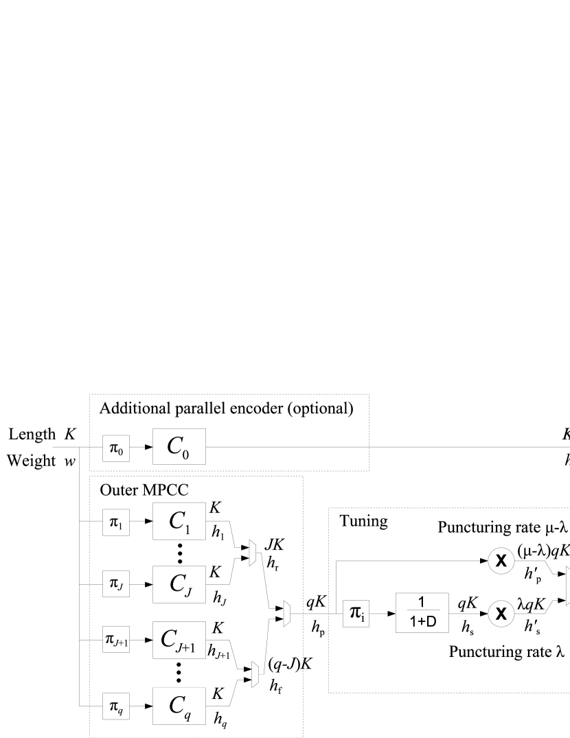
The output of the outer MPCC enters the serially concatenated inner accumulator, whose output weight is denoted by $h_{\mathrm{s}}$. Both the output of the outer MPCC and the output of the inner accumulator are punctured, then multiplexed together and passed to the channel. The puncturing rates $(\mu-\lambda)$ and $\lambda$ in Fig. 1 denote the fraction of bits that survive after puncturing the outer MPCC and the inner accumulator, and $h_{p}^{\prime}$ and $h_{s}^{\prime}$ are the corresponding weights, respectively. Finally, $h=h_{\mathrm{s}}^{\prime}+h_{\mathrm{p}}^{\prime}+h_{0}$ represents the total output codeword weight.

The parameter $\mu$ is used to control the rate of the TTC ensemble, i.e., considering the multiplexed output of the outer MPCC and inner accumulator, a total fraction of $\mu$ bits survive puncturing. The rate of the overall ensemble is thus given by

$$R=\frac{K}{N}=\frac{1}{\mu q+\mathcal{I}_{0}},$$ (1)

where $K$ is the input length, $N$ is the total output length, and $\mathcal{I}_{0}=1$ if there is an additional parallel encoder and $\mathcal{I}_{0}=0$ otherwise. As additional parallel encoders we consider FFCEs or simply a systematic branch.

Tuning the asymptotic minimum distance growth rate and the iterative decoding convergence threshold is done by varying the puncturing rate $\lambda$, i.e., changing the fraction of bits that come from the output of the inner serially concatenated accumulator. For $\lambda=0$, all the bits of the inner accumulator are punctured and the output is the (possibly punctured) output of the MPCC. For $\lambda=\mu$ on the other hand, all output bits of the tuning section stem from the inner accumulator and none of the bits of the outer MPCC survive puncturing.

In the sections of the paper that feature numerical results, from Subsection IV-B onwards, we consider four different types of TTCs, which are depicted in Fig. 2. For each type, we consider a version with only 2-state component encoders and a version with 4-state RCEs in the outer MPCC. All types are based on the rate $R=1/4$ HCCs introduced in [10] and, for $\lambda=\mu=1$, are identical to the HCC in [10], while for $\lambda=0$, we obtain the (possibly punctured) outer MPCC plus the optional parallel encoder.

Figure 2: Encoder structure for different TTC types with feedforward and recursive convolutional component encoders (FFCEs and RCEs, respectively).

The type 1 and 2 TTC ensembles have a rate $R=1/4$ outer MPCC with no additional parallel encoder ${\mathcal{C}}_{0}$ (see Fig. 2). While the outer MPCC of the type 1 ensemble consists of four identical rate-1 RCEs, the last encoder ${\mathcal{C}}_{4}$ of the MPCC in the type 2 ensemble is the 2-state FFCE having generator $[3]_{8}$ (in octal notation). The type 3 and 4 TTC ensembles have a rate $R=1/3$ outer MPCC consisting of three identical rate-1 RCEs plus an additional parallel encoder ${\mathcal{C}}_{0}$. In the type 3 ensemble, ${\mathcal{C}}_{0}$ is the $[3]_{8}$ FFCE, while in the type 4 ensemble it is simply a systematic branch. Thus, for $\mu=1$ and $\lambda=0$, when the output of the outer MPCC is not punctured and all bits from the inner encoder are punctured, the type 2 and 3 code ensembles are identical, while they differ for all other values of $\mu$ and $\lambda$. The outer MPCC of the type 2 ensemble (with 2-state encoders) was introduced in [15] and exhibits excellent iterative decoding behavior due to the presence of the FFCE (see [16]). In all the cases considered in this paper, the 2-state rate-1 RCEs are accumulators with generator $[1/3]_{8}$ and the 4-state RCEs are chosen to have the generator $[5/7]_{8}$.

We decode TTCs iteratively, in a component code oriented fashion, which is a generalization of the turbo-decoding principle applied in [1]. Component decoders employ maximum a posteriori probability (MAP) decoding strategies and the extrinsic information of one component decoder becomes a priori information for the other decoders. In our simulations we assume a straightforward iteration schedule, where each component decoder is activated once per iteration.

Since we use iterative decoding and not a MAP decoder for the overall code, the performance of the decoder in the moderate-to-high SNR region of the additive white Gaussian noise (AWGN) channel is greatly influenced but not solely determined by the minimum Hamming distance of the code. Pseudo-codewords and trapping sets also play a role in the error floor performance of the decoder (see, e.g. [17, 11]).

TTC ensembles with 2-state component encoders are closely related to LDPC codes and can also be decoded using the sum-product algorithm [18], so it is likely that the pseudo-weight properties of TTCs are similar to those of LDPC codes. In [19] it was shown that the minimum AWGN channel pseudo-weight of regular LDPC codes grows at best sub-linearly with block length, even though the minimum Hamming distance grows linearly with block length. There exist, however, specially constructed code ensembles where the minimum binary symmetric channel pseudo-weight can grow linearly with block length [20].

Since the minimum Hamming distance is an upper bound on the minimum pseudo-weight, we expect that designing TTC ensembles whose minimum distance grows linearly with block length will lead to code ensembles that also possess good pseudo-weight properties. This expectation is supported by the finite length (Hamming) distance analysis in Section IV and the simulation results in Section VII, both of which show that code ensembles with large minimum Hamming distance exhibit low error floors.

III Preliminaries

III-A Weight Enumerators

The weight spectrum of an $(N,K)$ linear encoder ${\mathcal{C}}(N)$ is described by its weight enumerator (WE) $A^{{\mathcal{C}}(N)}_{h}$, which specifies the number of codewords with output weight $h$. Likewise, let $A^{{\mathcal{C}}(N)}_{w,h}$ denote the input-output weight enumerator (IOWE), which specifies the number of codewords with input weight $w$ and output weight $h$. To investigate the distance properties of tuned turbo code ensembles, we consider the ensemble average of the above quantities. For an encoder ensemble $\mathbf{C}(N)$ of length $N$, we write the average IOWE as

$$\bar{A}^{\mathbf{C}(N)}_{w,h}=\frac{1}{|\mathbf{C}(N)|}\sum_{{\mathcal{C}}(N)\in\mathbf{C}(N)}A^{{\mathcal{C}}(N)}_{w,h},$$ (2)

where $|\mathbf{C}(N)|$ denotes the size of $\mathbf{C}(N)$. When the members of $\mathbf{C}(N)$ are equally likely, we obtain the average WE as

$$\bar{A}^{\mathbf{C}(N)}_{h}=\sum_{w=1}^{K}\bar{A}^{\mathbf{C}(N)}_{w,h}.$$ (3)

The average WE represents the expected number of codewords of weight $h$ if a code is randomly chosen from the ensemble $\mathbf{C}(N)$. In the rest of the paper, whenever the context is clear, we will omit the parameter $N$.

To obtain the average WE $\bar{A}^{\mathbf{C}_{\mathrm{TTC}}(N)}_{h}$ of TTC ensembles, we use the uniform interleaver analysis introduced in [21]. The uniform interleaver is a probabilistic device that maps an input block of weight $w$ and length $K_{\mathcal{C}}$ into all its possible $\binom{K_{\mathcal{C}}}{w}$ permutations with equal probability, thus decoupling the component encoders in a concatenated code and creating a code ensemble with equally likely members. An $(N_{\mathcal{C}},K_{\mathcal{C}})$ component encoder ${\mathcal{C}}(N_{\mathcal{C}})$, preceded by a uniform interleaver, results in the input-output weight distribution (IOWD)

$$\mathbb{P}^{{\mathcal{C}}(N_{\mathcal{C}})}_{w,h}=\frac{A^{{\mathcal{C}}(N_{\mathcal{C}})}_{w,h}}{\binom{K_{\mathcal{C}}}{w}},$$ (4)

where $\mathbb{P}^{{\mathcal{C}}(N_{\mathcal{C}})}_{w,h}$ is the probability that encoder ${\mathcal{C}}(N_{\mathcal{C}})$ transforms an input of weight $w$ into an output of weight $h$. For $(N_{\mathcal{C}},N_{\mathcal{C}})$ 2-state component encoders, the IOWE can be given in closed form as [22]

$${A}_{w,h}^{\mathrm{Acc}(N_{\mathcal{C}})}={A}^{\mathrm{FF}(N_{\mathcal{C}})}_{h,w}={\binom{N_{\mathcal{C}}-h}{\left\lfloor w/2\right\rfloor}\binom{h-1}{\left\lceil w/2\right\rceil-1}},$$ (5)

where $w/2\leq h\leq N_{\mathcal{C}}-w/2$, “Acc” represents the accumulator, and “FF” represents the 2-state FFCE with generator $[3]_{8}$.

In the case of TTCs, component codes may be punctured. The IOWE of punctured accumulators was analyzed in [23] by considering the serial concatenation of an accumulator and a single-parity-check. Using this approach, only regular puncturing patterns and puncturing rates of $\lambda=1/i$ with $i\in\mathbb{N}$ can be realized. To be able to vary $\lambda$ continuously, we therefore consider random puncturing, and the code ensembles we analyze are formed over all interleaver realizations, as well as over all possible puncturing patterns. Using random puncturing, the probability that a codeword of length $N$ and weight $h$ before puncturing is punctured to a codeword of length $N^{\prime}=\lambda N$ and weight $h^{\prime}$ is given by the hypergeometric distribution

$$\mathbb{P}^{\mathrm{P}(N^{\prime})}_{h,h^{\prime},\lambda}=\frac{\binom{N^{\prime}}{h^{\prime}}\binom{N-N^{\prime}}{h-h^{\prime}}}{\binom{N}{h}},$$ (6)

where (6) represents the IOWD of the random puncturing operation and we require $h^{\prime}\leq N^{\prime}$, $h-h^{\prime}\leq N-N^{\prime}$, and $h^{\prime}\leq h$. Throughout the paper we define the binomial coefficient $\binom{n}{k}$ to be zero if $n<k$.

The average component input-output weight enumerator (CIOWE) of an $(N,K)$ TTC, $\bar{A}_{w,h_{0},h_{1},\ldots,h_{q},h_{\mathrm{s}},h_{\mathrm{p}}^{\prime},h_{\mathrm{s}}^{\prime}}^{\mathbf{C}_{\mathrm{TTC}}(N)}$, is the average number of codewords with fixed input and output weights $w,h_{0},h_{1},\ldots,h_{q},h_{\mathrm{s}},h_{\mathrm{p}}^{\prime},$ and $h_{\mathrm{s}}^{\prime}$ of each component encoder in the TTC. The CIOWE is simply the product of the IOWDs of the components times the number of permutations of the input sequence, i.e.,

$$\bar{A}_{w,h_{0},h_{1},\ldots,h_{q},h_{\mathrm{s}},h_{\mathrm{p}}^{\prime},h_{\mathrm{s}}^{\prime}}^{\mathbf{C}_{\mathrm{TTC}}(N)}=$$ (7)

$$\binom{K}{w}\left(\prod_{i=0}^{q}\mathbb{P}_{w,h_{i}}^{{\mathcal{C}}_{i}(K)}\right)\cdot\mathbb{P}_{h_{\mathrm{p}},h_{\mathrm{s}}}^{\mathrm{Acc}(qK)}\cdot\mathbb{P}_{h_{\mathrm{p}},h_{\mathrm{p}}^{\prime},\mu-\lambda}^{\mathrm{P}(qK(\mu-\lambda))}\cdot\mathbb{P}_{h_{\mathrm{s}},h_{\mathrm{s}}^{\prime},\lambda}^{\mathrm{P}(qK\lambda)},$$

where we denote the total output weight of the outer MPCC as $h_{\mathrm{p}}=\sum_{i=1}^{q}h_{i}$. If there is no additional parallel encoder, we define $\mathbb{P}^{{\mathcal{C}}_{0}(K)}_{w,h_{0}}$ to be one for $h_{0}=0$ and zero otherwise.

The ensemble average IOWE of a TTC, $\bar{A}_{w,h}^{\mathbf{C}_{\mathrm{TTC}}(N)}$, is then the summation over all CIOWEs such that the codeword has weight $h$. To include the total output weight $h$ in the CIOWE, we represent the punctured weight of the inner serial accumulator as $h_{\mathrm{s}}^{\prime}=h-h_{\mathrm{p}}^{\prime}-h_{0}$, thus obtaining the IOWE

$$\bar{A}_{w,h}^{\mathbf{C}_{\mathrm{TTC}}(N)}=$$ (8)

$$\sum_{h_{0}=\mathcal{I}_{0}}^{K}\sum_{h_{1}=1}^{K}\cdots\sum_{h_{q}=1}^{K}\sum_{h_{\mathrm{s}}=1}^{qK}\sum_{h_{\mathrm{p}}^{\prime}=0}^{h}\bar{A}_{w,h_{0},h_{1},\ldots,h_{q},h_{\mathrm{s}},h_{\mathrm{p}}^{\prime},h}^{\mathbf{C}_{\mathrm{TTC}}(N)}.$$

Note that, with random puncturing, it is possible that all the weight is punctured and therefore the enumeration of punctured weights starts at zero.

III-B The Spectral Shape

To investigate the asymptotic minimum distance properties of tuned turbo codes as the block length $N$ tends to infinity, we will make use of the asymptotic spectral shape function originally introduced by Gallager [24],

$$r(\rho)=\limsup_{N\rightarrow\infty}\frac{\ln\bar{A}^{\mathbf{C}(N)}_{\left\lfloor\rho N\right\rfloor}}{N},$$ (9)

where $\rho=\frac{h}{N}$ is the normalized codeword weight. The spectral shape is the exponential part of the average WE normalized by the block length $N$. When $r(\rho)<0$, the average number of codewords with normalized weight $\rho$ goes exponentially to zero as $N$ tends to infinity. When $r(\rho)>0$, on the other hand, the average number of codewords with normalized weight $\rho$ grows exponentially in $N$. When $r(\rho)=0$, the average number of codewords with normalized weight $\rho$ does not exhibit exponential growth — it might increase or decrease polynomially, for example.

Similarly, we define the asymptotic IOWD of an $(N_{\mathcal{C}},K_{\mathcal{C}})$ component code ${\mathcal{C}}(N_{\mathcal{C}})$ as

$$f^{{\mathcal{C}}}_{\alpha,\beta}=\lim_{N_{\mathcal{C}}\to\infty}\frac{\ln\mathbb{P}_{\left\lfloor\alpha K_{\mathcal{C}}\right\rfloor,\left\lfloor\beta N_{\mathcal{C}}\right\rfloor}^{{\mathcal{C}}(N_{\mathcal{C}})}}{N_{\mathcal{C}}},$$ (10)

where $\alpha$ and $\beta$ are the normalized input and output weight w.r.t. the input block length $K_{\mathcal{C}}$ and the output block length $N_{\mathcal{C}}$, respectively, of code ${\mathcal{C}}(N_{\mathcal{C}})$. Stirling’s approximation can be used to bound the binomial coefficients as

$$\frac{e^{n{\mathbb{H}}\left(k/n\right)}}{n+1}\leq\binom{n}{k}\leq e^{n{\mathbb{H}}\left(k/n\right)},$$ (11)

where ${\mathbb{H}}\left(x\right)=-x\ln x-(1-x)\ln(1-x)$ denotes the binary entropy function using the natural logarithm.

Using (4), (5), (10), and (11) the asymptotic IOWD of the accumulator is given by

$$f^{\mathrm{Acc}}_{\alpha,\beta}=(1-\beta){\mathbb{H}}\left(\frac{\alpha}{2(1-\beta)}\right)+\beta{\mathbb{H}}\left(\frac{\alpha}{2\beta}\right)-{\mathbb{H}}\left(\alpha\right),$$ (12)

where $\alpha=w/N_{\mathcal{C}}$ and $\beta=h/N_{\mathcal{C}}$ (see also [5]). In the same way, the asymptotic IOWD of the 2-state FFCE is given by

$$f^{\mathrm{FF}}_{\alpha,\beta}=(1-\alpha){\mathbb{H}}\left(\frac{\beta}{2(1-\alpha)}\right)+\alpha{\mathbb{H}}\left(\frac{\beta}{2\alpha}\right)-{\mathbb{H}}\left(\alpha\right).$$ (13)

Similarly, by using (6), (10), and (11), the asymptotic IOWD of the random puncturing operation is given by

$$f^{\mathrm{P}}_{\beta,\beta^{\prime},\lambda}={\mathbb{H}}\left(\beta^{\prime}\right)+\frac{1-\lambda}{\lambda}{\mathbb{H}}\left(\frac{\beta-\lambda\beta^{\prime}}{1-\lambda}\right)-\frac{1}{\lambda}{\mathbb{H}}\left(\beta\right),$$ (14)

where $\beta=h/N_{\mathcal{C}}$ and $\beta^{\prime}=h^{\prime}/(\lambda N_{\mathcal{C}})$.

We now define the asymptotic CIOWE of an $(N,K)$ TTC as

$$\mathcal{F}_{\alpha,\rho_{0},\rho_{1},\ldots,\rho_{q},\rho_{\mathrm{s}},\rho_{\mathrm{p}}^{\prime},\rho}^{\mathbf{C}_{\mathrm{TTC}}}=\lim_{N\rightarrow\infty}\frac{\ln\bar{A}_{w,h_{0},h_{1},\ldots,h_{q},h_{\mathrm{s}},h_{\mathrm{p}}^{\prime},h}^{\mathbf{C}_{\mathrm{TTC}}(N)}}{N},$$ (15)

where $\alpha=w/K$, $\rho_{i}=h_{i}/K$, $i=0,1,\ldots,q$, $\rho_{\mathrm{s}}=h_{\mathrm{s}}/(qK)$, $\rho_{\mathrm{p}}^{\prime}=h_{\mathrm{p}}^{\prime}/(q(\mu-\lambda)K)$, and $\rho=h/(q\mu+\mathcal{I}_{0})K=h/N$. Using (15), we rewrite the asymptotic spectral shape as the optimization problem

$$r(\rho)=\sup_{\alpha,\rho_{0},\ldots,\rho_{\mathrm{p}}^{\prime}}\mathcal{F}_{\alpha,\rho_{0},\rho_{1},\ldots,\rho_{q},\rho_{\mathrm{s}},\rho_{\mathrm{p}}^{\prime},\rho}^{\mathbf{C}_{\mathrm{TTC}}}.$$ (16)

We obtain the asymptotic CIOWE of a TTC by inserting its CIOWE (7) into (15). The logarithm transforms the product of IOWDs in (7) into a sum, and in the limit as the block lengths of each component code $N_{{\mathcal{C}}_{i}}$ tend to infinity, the asymptotic CIOWE of a TTC can be written in terms of the asymptotic IOWDs of its component codes, weighted by their respective block lengths divided by $N$, as

$$\mathcal{F}_{\alpha,\rho_{0},\rho_{1},\ldots,\rho_{q},\rho_{\mathrm{s}},\rho_{\mathrm{p}}^{\prime},\rho}^{\mathbf{C}_{\mathrm{TTC}}}=$$ (17)

$$qR\left(\frac{1}{q}{\mathbb{H}}\left(\alpha\right)+\frac{1}{q}\sum_{i=0}^{q}f^{{\mathcal{C}}_{i}}_{\alpha,\rho_{i}}+f^{\mathrm{Acc}}_{\rho_{\mathrm{p}},\rho_{\mathrm{s}}}+\right.$$

$$\left.(\mu-\lambda)f^{\mathrm{P}}_{\rho_{\mathrm{p}},{\rho^{\prime}}_{\mathrm{p}},(\mu-\lambda)}+\lambda f^{\mathrm{P}}_{\rho_{\mathrm{s}},\rho_{\mathrm{s}}^{\prime},\lambda}\right),$$

where $\rho_{\mathrm{p}}=h_{\mathrm{p}}/qK$ and $R=K/N$ is the rate of the TTC given by (1). To include the normalized total output weight $\rho=h/N$ in the asymptotic CIOWE, we represent the normalized punctured weight of the inner serial accumulator $\rho_{\mathrm{s}}^{\prime}$ as

$$\rho_{\mathrm{s}}^{\prime}= \,\frac{h_{\mathrm{s}}^{\prime}}{q\lambda K}=\frac{h-h_{\mathrm{p}}^{\prime}-h_{0}}{q\lambda K}$$ (18)

$$= \frac{\rho/R-q(\mu-\lambda){\rho_{\mathrm{p}}}^{\prime}-\rho_{0}}{q\lambda}.$$

If there is some $\hat{\rho}>0$ such that $r(\rho)<0$ for all $0<\rho<\hat{\rho}$, we would immediately have that $\hat{\rho}$ is the asymptotic growth rate of the minimum distance of the ensemble. However, this is not the case for TTCs.

Proposition 1.

For $0\leq\rho<Rq\lambda$, the spectral shape of a TTC cannot be negative but is lower bounded by $r(\rho)=0$.

Proof:

The proposition is trivially proved by setting $\rho_{\mathrm{p}}=0$ (which implies $\alpha=0$, $\rho_{0}=0$, $\rho_{i}=0$ for $i=1,\ldots,q$, and $\rho_{\mathrm{p}}^{\prime}=0$) and $\rho_{\mathrm{s}}=\rho_{\mathrm{s}}^{\prime}=\rho/({Rq\lambda})$. Setting $\rho_{\mathrm{p}}=0$ results in the asymptotic IOWDs of the 2-state component encoders (12), (13) in the CIOWE of a TTC to be zero and setting $\rho_{\mathrm{s}}=\rho_{\mathrm{s}}^{\prime}$ results in the asymptotic IOWD of the random puncturing operation (14) to be zero, resulting in

$$\mathcal{F}_{0,0,0,\ldots,0,(\rho/({Rq\lambda})),0,\rho}^{\mathbf{C}_{\mathrm{TTC}}}=0.$$

∎

Thus, it cannot be directly concluded that the resulting ensembles are asymptotically good, but we will show in the next section that the 2-state ensembles are indeed asymptotically good and we conjecture the same for the 4-state ensembles.

IV Minimum Distance Analysis

In this section we make use of the expressions from the previous section to perform both an asymptotic and a finite length minimum distance analysis of tuned turbo codes with 2-state component encoders.

IV-A Asymptotic Analysis

For a TTC with $q$ encoders and $J$ accumulators in the outer MPCC (see Fig. 1), the probability that a randomly chosen code from the ensemble has minimum distance $d_{\mathrm{min}}<d$ is upper bounded by

$${\mathbb{P}}\left(d_{\mathrm{min}}<d\right)\leq(\bar{A}_{0}^{\mathbf{C}_{\mathrm{TTC}}(N)}-1)+\sum_{h=1}^{d-1}\bar{A}_{h}^{\mathbf{C}_{\mathrm{TTC}}(N)}$$ (19)

$$=\sum_{w=1}^{K}\sum_{h_{0}={\mathcal{I}}_{0}}^{K}\sum_{h_{1}=1}^{K}\cdots\sum_{h_{q}=1}^{K}\sum_{h_{\mathrm{s}}=1}^{Kq}\sum_{h_{\mathrm{p}}^{\prime}=0}^{\lfloor Kq(\mu-\lambda)\rfloor}\sum_{h=0}^{d-1}\bar{A}_{w,h_{0},h_{1},\ldots,h_{q},h_{\mathrm{s}},h_{\mathrm{p}}^{\prime},h}^{\mathbf{C}_{\mathrm{TTC}}(N)}.$$ (20)

Note that, while the average number of all-zero codewords $\bar{A}_{0}^{\mathbf{C}(N)}$ equals $1$ for unpunctured linear codes, with punctured codes there is a possibility that all the weight is removed by the puncturing operation. We take the probability of this event into account with the term $(\bar{A}_{0}^{\mathbf{C}_{\mathrm{TTC}}(N)}-1)$ in (19) and with the summation over $h$ starting from zero in (20), while the summation over $w$ starts at $w=1$.

We define the value $\hat{\rho}$ as follows.

Definition 1.

Let $0\leq\hat{\rho}<Rq\lambda/2$ be such that, for all $0\leq\rho<\hat{\rho}$, the unique supremum of the asymptotic CIOWE of TTCs given by (17) is achieved for $\rho_{\mathrm{p}}=0$ and $\rho_{\mathrm{s}}=\rho_{\mathrm{s}}^{\prime}=\rho/({Rq\lambda})$.

$$A_{2}\leq (NRq+1)^{q+5}\exp\left\{\max_{\stackrel{{\scriptstyle h_{\mathrm{p}}>h_{\mathrm{p}}^{*},h<\left\lceil N(\hat{\rho}-\epsilon)\right\rceil}}{{w,h_{0},h_{\mathrm{p}}^{\prime},h_{\mathrm{s}}}}}N\cdot\mathcal{F}^{{\mathcal{C}}_{\mathrm{TTC}}}_{\frac{w}{NR},\,\frac{h_{0}}{NR},\,\frac{h_{1}}{NRq},\,\ldots,\,\frac{h_{q}}{NRq},\,\frac{h_{\mathrm{s}}}{NRq},\,\frac{h_{\mathrm{p}}^{\prime}}{NRq(\mu-\lambda)},\,\frac{h}{N}}+(2q+8)\ln(NRq+1)\right\}$$ (24)

$$= \exp\left\{\max_{\stackrel{{\scriptstyle h_{\mathrm{p}}>h_{\mathrm{p}}^{*},h<\left\lceil N(\hat{\rho}-\epsilon)\right\rceil}}{{w,h_{0},h_{\mathrm{p}}^{\prime},h_{\mathrm{s}}}}}N\cdot\mathcal{F}^{{\mathcal{C}}_{\mathrm{TTC}}}_{\frac{w}{NR},\,\frac{h_{0}}{NR},\,\frac{h_{1}}{NRq},\,\ldots,\,\frac{h_{q}}{NRq}\frac{h_{\mathrm{s}}}{NRq},\,\frac{h_{\mathrm{p}}^{\prime}}{NRq(\mu-\lambda)},\,\frac{h}{N}}+(3q+13)\ln(NRq+1)\right\}$$

Following the procedure established in [25] and [7], we can split (20) into two parts, $A_{1}$ and $A_{2}$, depending on the output weight of the outer MPCC $h_{\mathrm{p}}=\sum_{i=1}^{q}h_{i}$. For any positive integer $h_{\mathrm{p}}^{*}$, $q\leq h_{\mathrm{p}}^{*}\leq Kq$, we can write

$${\mathbb{P}}\left(d_{\mathrm{min}}<d\right)=$$ (21)

$$\underbrace{{\mathbb{P}}\left(d_{\mathrm{min}}<d\cap h_{\mathrm{p}}\leq h_{\mathrm{p}}^{*}\right)}_{A_{1}}+\underbrace{{\mathbb{P}}\left(d_{\mathrm{min}}<d\cap h_{\mathrm{p}}>h_{\mathrm{p}}^{*}\right)}_{A_{2}}.$$

We now proceed to show that, with appropriately chosen values of $h_{\mathrm{p}}^{*}$ and $d$, $A_{1}\rightarrow 0$ and $A_{2}\rightarrow 0$ as $N\rightarrow\infty$ for all $d<\left\lceil N(\hat{\rho}-\epsilon)\right\rceil$, where $\epsilon>0$ is an arbitrarily small constant, which implies that the ensemble is asymptotically good with asymptotic minimum distance growth rate $\hat{\rho}$.

Lemma 1.

As $N\rightarrow\infty$, for all $J>2$ and $h_{\mathrm{p}}^{*}\leq N^{\frac{J-2}{J}-\epsilon}$, we have

$$A_{1}={\mathbb{P}}\left(d_{\mathrm{min}}<\left\lceil N(\hat{\rho}-\epsilon)\right\rceil\cap h_{\mathrm{p}}\leq h_{\mathrm{p}}^{*}\right)\rightarrow 0$$ (22)

for arbitrarily small values of $\epsilon>0$.

Proof:

Using the simple upper bound

$$A_{1}= {\mathbb{P}}\left(d_{\mathrm{min}}<\left\lceil N(\hat{\rho}-\epsilon)\right\rceil\cap h_{\mathrm{p}}\leq h_{\mathrm{p}}^{*}\right)$$

$$\leq{\mathbb{P}}\left(h_{\mathrm{p}}\leq h_{\mathrm{p}}^{*}\right),$$

the problem is reduced to finding the asymptotic minimum distance of an MPCC with $J$ parallel concatenated RCEs, which was lower bounded in [3] and [25] as

$$\mathbb{P}\left(h_{\mathrm{p}}\leq N^{\frac{J-2}{J}-\epsilon}\right)\leq C_{1}\cdot N^{-\epsilon/2}$$

for arbitrarily small values of $\epsilon>0$, some positive constant $C_{1}$, and $N$ sufficiently large. ∎

Now, considering $A_{2}$, we upper bound the $q+5$ sums in (20) by their maximum element times $NRq+1$, which is an upper bound on the number of terms in each sum, and we obtain

$$A_{2}= {\mathbb{P}}\left(d_{\mathrm{min}}<\left\lceil N(\hat{\rho}-\epsilon)\right\rceil\cap h_{\mathrm{p}}>h_{\mathrm{p}}^{*}\right)$$ (23)

$$\leq (NRq+1)^{q+5}\max_{\begin{subarray}{c}\sum_{i=1}^{q}h_{i}=h_{\mathrm{p}}>h_{\mathrm{p}}^{*}\\ h<\left\lceil N(\hat{\rho}-\epsilon)\right\rceil\\ w,h_{0},h_{\mathrm{p}}^{\prime},h_{\mathrm{s}}\end{subarray}}\bar{A}_{w,h_{0},h_{1},\ldots,h_{q},h_{\mathrm{s}},h_{\mathrm{p}}^{\prime},h}^{\mathbf{C}_{\mathrm{TTC}}(N)}.$$

Using Stirling’s approximation (11), we can upper bound each of the $q+4$ IOWDS in the CIOWE of (7) as

$$\mathbb{P}_{w_{i},h_{i}}^{{\mathcal{C}}_{i}(N_{{\mathcal{C}}_{i}})}\leq\exp\left\{N_{{\mathcal{C}}_{i}}f_{\alpha_{i},\beta_{i}}^{{\mathcal{C}}_{i}}+2\ln(N_{{\mathcal{C}}_{i}}+1)\right\}.$$

Then using the notation of the asymptotic CIOWE (17) and upper bounding $N_{{\mathcal{C}}_{i}}+1$ by $NRq+1$, we obtain (24).

Thus, to bound $A_{2}$ it is necessary to examine the asymptotic CIOWE and the asymptotic spectral shape (16) of TTCs. We now show that if there exists a $\hat{\rho}>0$ as defined in Definition 1, we have $A_{2}\rightarrow 0$ as $N\rightarrow\infty$. To this end we make use of the log-concavity of the IOWDs of the component encoders.

Proposition 2.

It holds that:

1. For a fixed input weight $w$, the IOWD $\mathbb{P}_{w,h}^{\mathrm{Acc}(N_{\mathcal{C}})}$ of the accumulator forms a logarithmically concave sequence in the output weight $h$ and its maximum occurs at $h=N_{\mathcal{C}}/2$.

2. For a fixed input weight $w$, the IOWD $\mathbb{P}_{w,h}^{\mathrm{FF}}{(N_{\mathcal{C}})}$ of the 2-state FFCE forms a logarithmically concave sequence in the output weight $h$ and its maximum occurs at $h=2w(1-w/{N_{\mathcal{C}}})$.

3. For a fixed input weight $h$, the IOWD $\mathbb{P}_{h,h^{\prime},\lambda}^{\mathrm{P}(N^{\prime})}$ of the random puncturing operation forms a strictly logarithmically concave sequence in the output weight $h^{\prime}$ and its maximum occurs at $h^{\prime}=\lambda h$.

The proofs of these statements can be found in Appendix A. From Proposition 2 it follows that, for a fixed input weight $w$ and a fixed total output weight of the RCEs $h_{\mathrm{r}}=\sum_{i=1}^{J}h_{i}$ (see Fig. 1), the CIOWE of TTCs is maximized when the RCEs in the outer MPCC contribute equally to $h_{\mathrm{r}}$, i.e., when $h_{i}=h_{\mathrm{r}}/J$, or $\rho_{\mathrm{i}}=h_{\mathrm{r}}/JK=\rho_{\mathrm{r}}$, $i\in\{1,\ldots,J\}$. Equivalently, the CIOWE of TTCs is maximized when the FFCEs in the outer MPCC contribute equally to $h_{\mathrm{f}}$, i.e., when $h_{i}=h_{\mathrm{f}}/(q-J)$, or $\rho_{i}=h_{\mathrm{f}}/(q-J)K=\rho_{\mathrm{f}}$, $i\in\{J+1,\ldots,q\}$. Thus we can substitute $\rho_{\mathrm{s}}$ and $\rho_{\mathrm{f}}$ for the $\rho_{i}$ in the asymptotic CIOWE and the number of variables in the maximization problem in (24) is reduced. The normalized output weight of the outer MPCC is then given by $\rho_{\mathrm{p}}=(J\rho_{\mathrm{s}}/q+(q-J)\rho_{\mathrm{f}}/q)$.

Lemma 2.

If there exists a $\hat{\rho}>0$ then for $J>2$ RCEs in the outer MPCC and

$$\lim_{n\rightarrow\infty}\frac{\ln(NRq+1)}{h^{*}_{\mathrm{p}}}=0$$

we have

$$A_{2}={\mathbb{P}}\left(d_{\mathrm{min}}<\left\lceil N(\hat{\rho}-\epsilon)\right\rceil\cap h_{\mathrm{p}}>h_{\mathrm{p}}^{*}\right)\rightarrow 0$$

as $N\rightarrow\infty$, where $\epsilon>0$ is an arbitrarily small constant.

Proof:

We investigate the asymptotic CIOWE (17) in the region $0\leq\rho<\hat{\rho}$ by splitting it into two parts, $RqF_{1}$ and $RqF_{2}$, and write

$$N\cdot\mathcal{F}^{{\mathcal{C}}_{\mathrm{TTC}}}_{\frac{w}{NR},\,\frac{h_{0}}{NR},\,\frac{h_{\mathrm{s}}}{NRJ},\,\frac{h_{\mathrm{f}}}{NR(q-J)},\,\frac{h_{\mathrm{r}}}{NRq},\,\frac{h_{\mathrm{p}}^{\prime}}{NRq(\mu-\lambda)},\,\frac{h}{N}}=NRq(F_{1}+F_{2})$$ (25)

with

$$F_{1}= \frac{1}{q}{\mathbb{H}}\left(\frac{w}{NR}\right)+\frac{{\mathcal{I}}_{0}}{q}f^{{\mathcal{C}}_{0}}_{\frac{w}{NR},\,\frac{h_{0}}{NR}}+\frac{J}{q}f^{\mathrm{Acc}}_{\frac{w}{NR},\,\frac{h_{\mathrm{r}}}{NRJ}}$$ (26)

$$+\frac{q-J}{q}f^{\mathrm{FF}}_{\frac{w}{NR},\,\frac{h_{\mathrm{f}}}{NR(q-J)}}+f^{\mathrm{Acc}}_{\frac{h_{\mathrm{p}}}{NRq},\,\frac{h_{\mathrm{s}}}{NRq}}$$

$$F_{2}=(\mu-\lambda)f^{\mathrm{P}}_{\frac{h_{\mathrm{p}}}{NRq},\,\frac{h_{\mathrm{p}}^{\prime}}{NRq(\mu-\lambda)},\,\mu-\lambda}+\lambda f^{\mathrm{P}}_{\frac{h_{\mathrm{s}}}{NRq},\,\frac{h-h_{\mathrm{p}}^{\prime}-h_{0}}{NR\lambda q},\,\lambda}.$$ (27)

The term $F_{1}$ includes the asymptotic IOWDs of the encoders, whereas $F_{2}$ includes the asymptotic IOWDs of the random puncturing operation. From Definition 1 we have that, for $0\leq\rho<\hat{\rho}$, the spectral shape has its supremum at $r(\rho)=0$, which is achieved for $\rho_{p}=0$ and $\rho_{s}=\rho_{s}^{\prime}=\rho/(Rq\lambda)$.

First we note that $F_{2}\leq 0$, with $F_{2}=0$ for $\rho_{s}=\rho_{s}^{\prime}$ and $F_{2}<0$ otherwise (see the proof of part 3 of Proposition 2), so we can simply upper bound the term $NRqF_{2}$ by zero.

Next we note that $F_{1}$ tends to zero for $\rho_{\mathrm{p}}\rightarrow 0$ (see the proof of Proposition 1), and hence to upper bound $NRqF_{1}$ we consider all possible $h_{\mathrm{p}}>h_{\mathrm{p}}^{*}$ such that $\rho_{\mathrm{p}}$ tends asymptotically to zero, i.e.,

$$\lim_{N\rightarrow\infty}\frac{h_{\mathrm{p}}}{N}=0.$$

Then we have

$$\lim_{\begin{subarray}{c}N\rightarrow\infty\\ h_{\mathrm{p}}/N\rightarrow 0\end{subarray}}NRq\,F_{1}=\lim_{\begin{subarray}{c}N\rightarrow\infty\\ h_{\mathrm{p}}/N\rightarrow 0\end{subarray}}h_{\mathrm{p}}\cdot\frac{F_{1}}{\rho_{\mathrm{p}}}=h_{\mathrm{p}}\cdot\frac{d}{d\rho_{\mathrm{p}}}\left.F_{1}\right|_{\rho_{\mathrm{p}}=0},$$ (28)

where both $F_{1}$ and $\rho_{\mathrm{p}}=h_{\mathrm{p}}/(NRq)$ tend asymptotically to zero as $N\rightarrow\infty$ and the fraction $F_{1}/\rho_{\mathrm{p}}$ is the difference quotient of the point $F_{1}|_{\rho_{\mathrm{p}}=0}$, which as $N\rightarrow\infty$ yields the total derivative of $F_{1}$ with respect to $\rho_{\mathrm{p}}$ evaluated at $\rho_{\mathrm{p}}=0$.

We show in Appendix B that, if there exists a $\hat{\rho}>0$, then, for $J>2$ accumulators in the outer MPCC, the total derivative of $F_{1}$ with respect to $\rho_{\mathrm{p}}$ evaluated at $\rho_{\mathrm{p}}=0$ is bounded by

$$\frac{d}{d\rho_{\mathrm{p}}}\left.F_{1}\right|_{\rho_{\mathrm{p}}=0}\leq-C_{2},$$ (29)

for some positive constant $C_{2}$ and for $\rho_{\mathrm{s}}<1/2$.

So, for $\rho_{\mathrm{p}}=0$, from (24), (25), (26), (27), (28), and (29) we can write

$$A_{2}\leq\exp\left\{-C_{2}\cdot h_{\mathrm{p}}+(3q+13)\ln(NRq+1)\right\},$$ (30)

and $\lim_{N\rightarrow\infty}A_{2}=0$ for all $h_{\mathrm{p}}^{*}$ that satisfy $\lim_{N\rightarrow\infty}\ln(NRq+1)/h_{\mathrm{p}}^{*}=0$. ∎

Remark 1.

The fact that in Appendix B we require $\rho_{\mathrm{s}}<1/2$ for (29) to be negative together with the fact that we require $\rho_{s}=\rho_{s}^{\prime}=\rho/(Rq\lambda)$ for $F_{2}$ to be zero results in the upper bound on the asymptotic minimum distance growth rate

$$\hat{\rho}<\frac{Rq\lambda}{2}$$ (31)

given in Definition 1.

We summarize our results in the following Theorem.

Theorem 1.

If there exists a $\hat{\rho}>0$ as defined in Definiton 1 for a 2-state TTC ensemble with $J>2$ RCEs in the outer MPCC, then the 2-state TTC ensemble is asymptotically good and the asymptotic minimum distance growth rate is at least $\hat{\rho}$.

Proof:

From Lemmas 1 and 2 we have that, for an arbitrarily small constant $\epsilon>0$, both

$${\mathbb{P}}\left(d_{\mathrm{min}}<\left\lceil N(\hat{\rho}-\epsilon)\right\rceil\cap h_{\mathrm{p}}\leq h_{\mathrm{p}}^{*}\right)\rightarrow 0$$

and

$${\mathbb{P}}\left(d_{\mathrm{min}}<\left\lceil N(\hat{\rho}-\epsilon)\right\rceil\cap h_{\mathrm{p}}>h_{\mathrm{p}}^{*}\right)\rightarrow 0$$

as $N\rightarrow\infty$ for any $h_{\mathrm{p}}^{*}$ satisfying

$$\lim_{N\rightarrow\infty}\frac{\ln(NRq+1)}{h^{*}_{\mathrm{p}}}=0\quad\mathrm{and}\quad h^{*}_{\mathrm{p}}\leq N^{\frac{J-2}{J}-\epsilon}.$$

∎

Theorem 1 proves that $\hat{\rho}$ is a lower bound on the asymptotic minimum distance growth rate of a 2-state TTC ensemble. In a slight abuse of notation, from now on we refer to $\hat{\rho}$ as the asymptotic minimum distance growth rate.

IV-B Asymptotic Minimum Distance Growth Rates

While the spectral shapes of TTCs cannot be negative, the existence of a positive $\hat{\rho}$ according to Definition 1 implies that the ensemble is asymptotically good. As is common practice, we numerically evaluate the spectral shapes of TTC ensembles and use a subspace trust-region method [26] to evaluate the supremum of the asymptotic CIOWE. For 2-state component codes, the asymptotic IOWDs are available in closed form, but for 4-state ensembles, we cannot obtain closed form expressions, so to compute the asymptotic spectral shapes we use the method outlined in [27] to calculate them numerically.

Fig. 3 shows the asymptotic spectral shapes for the rate $R=1/4$ TTC ensembles with $\mu=\lambda=1$, i.e., the spectral shapes of the HCCs. The asymptotic spectral shape function of the entire ensemble of block codes is also shown. It crosses zero at the GVB for rate $R=1/4$. The ensembles with 2-state RCEs in the outer MPCC are plotted with solid lines, while the ensembles with 4-state RCEs in the outer MPCC are plotted with dashed lines. The spectral shapes are never negative, but they start out with a zero stretch and turn positive at the asymptotic distance growth rate $\hat{\rho}$.

Figure 3: Asymptotic spectral shapes for the rate $R=1/4$ TTCs with $\mu=\lambda=1$.

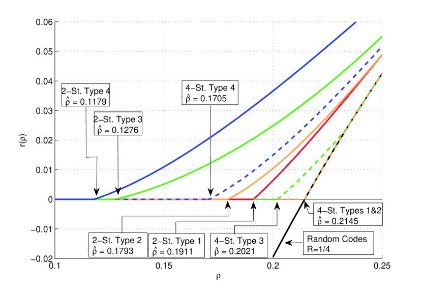
Among the 2-state ensembles, the type 1 scheme has the largest asymptotic distance growth rate of $\hat{\rho}=0.1911$. Replacing one of the parallel concatenated accumulators by its feedforward inverse (type 2) decreases the asymptotic distance growth rate to $\hat{\rho}=0.1793$. When only three branches enter the inner serially concatenated accumulator and the output of the $1+D$ branch is sent straight through to the channel (type 3), the asymptotic distance growth rate reduces further to $\hat{\rho}=0.1276$, and for the systematic type 4 scheme we obtain an asymptotic distance growth rate of only $\hat{\rho}=0.1179$.

Employing 4-state $[5/7]_{8}$ codes instead of accumulators in the outer MPCCs increases the asymptotic distance growth rates w.r.t. the 2-state ensembles. In the case of the type 1 and type 2 ensembles with 4-state encoders in the outer MPCCs, the positive part of the asymptotic spectral shape is practically indistinguishable from the spectral shape of the entire ensemble of block codes.

Figure 4: Asymptotic minimum distance growth rates of the type 1 TTC as the tuning parameter $\lambda$ varies, $0\leq\lambda\leq\mu$. In each case, the GVB is drawn only up to $\lambda=\mu$, the maximum possible value of $\lambda$.

Figure 5: Asymptotic minimum distance growth rates of the type 4 TTC as the tuning parameter $\lambda$ varies, $0\leq\lambda\leq\mu$. In each case, the GVB is drawn only up to $\lambda=\mu$, the maximum possible value of $\lambda$.

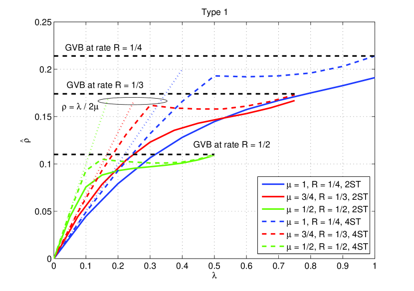
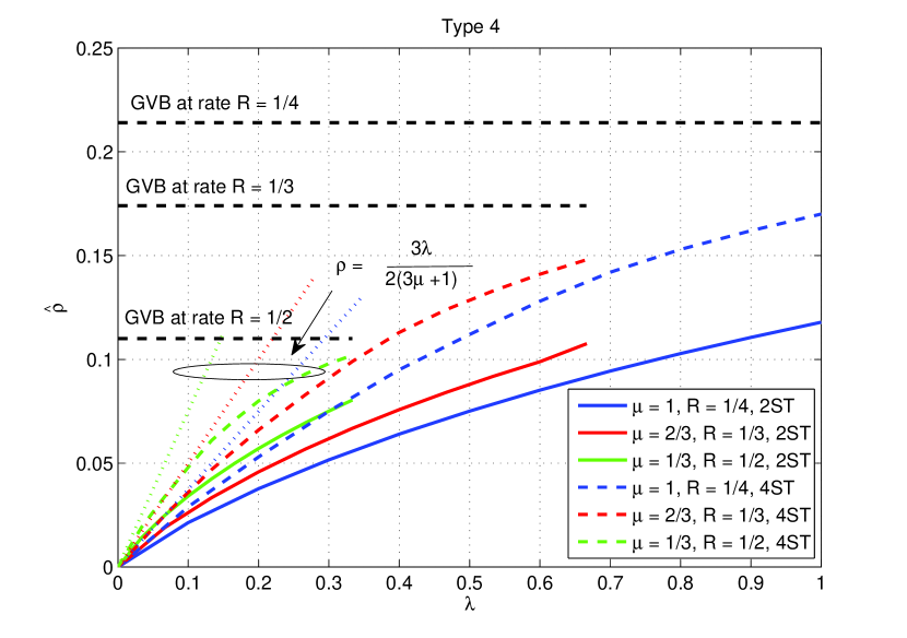
Fig. 4 shows the asymptotic minimum distance growth rates $\hat{\rho}$ of the type 1 TTC as the tuning parameter $\lambda$ varies, $0\leq\lambda\leq\mu$. As the code rate increases by reducing the coefficient $\mu$, the initial slope of the asymptotic distance growth rate curve becomes steeper. For small $\lambda$, these curves approach the upper bound on $\hat{\rho}$ given by (31) and indicated by the line $\hat{\rho}=\frac{\lambda}{2\mu}$ for the type 1 ensemble. This steep increase in the asymptotic distance growth rates with $\lambda$ is followed by the curve flattening out as the asymptotic distance growth rates approach the GVB. The green curve for the rate $R=1/2$ code ensemble shows the steepest increase (among the curves shown) but then flattens out around $\lambda=0.15$. Like the 4-state code ensembles it reaches the GVB for $\lambda=\mu$. The asymptotic distance growth rates of the type 2 tuned turbo code show the same general behavior, but they are smaller than those of the type 1 ensemble and the increase for small $\lambda$ is not as steep.

Type 3 and 4 TTCs also show the same general behavior, with the asymptotic distance growth rates of the type 3 ensemble being slightly larger than for the type 4 ensemble. The asymptotic distance growth rates of the type 4 ensemble are shown in Fig. 5. The initial slope of the curves is smaller than for the type 1 ensemble, and for $\lambda=\mu$ the asymptotic distance growth rates are further away from the GVB. They also increase more smoothly with $\lambda$ than for the type 1 ensemble.

IV-C Finite Length Analysis

The minimum distance of a TTC ensemble for a finite block length $N$ can also be analyzed using (19). In particular, if we set ${\mathbb{P}}\left({d_{\mathrm{min}}}<d\right)=\epsilon$, where $\epsilon$ is any positive value between $0$ and $1$, we expect that at least a fraction $1-\epsilon$ of the codes in the ensemble have a minimum distance ${d_{\mathrm{min}}}$ of at least $d$. In the following, we choose $\epsilon=1/2$, i.e., we expect that at least half of the codes in the ensemble have a ${d_{\mathrm{min}}}$ at least equal to the value predicted by the curves.

Figure 6: Lower bound on the minimum distance of the $R=1/4$ type 2 TTCs with 2-state component encoders (filled markers) and 4-state component encoders (empty markers) for $\mu=1$, $\epsilon=1/2$, and different values of the tuning parameter $\lambda$.

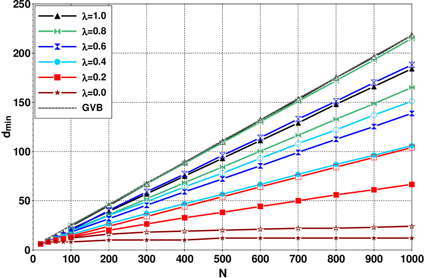
In Fig. 6 we show the lower bound on ${d_{\mathrm{min}}}$ versus the code block length $N$ for the $R=1/4$ type 2 tuned TTC ensembles with 2- and 4-state component encoders and several values of $\lambda$. The finite length GVB is also plotted for reference. The results are consistent with the asymptotic analysis in the previous section and show increasing minimum distance growth rates with increasing values of $\lambda$. Also, for a given value of the tuning parameter $\lambda$, the minimum distance of the type 2 code ensemble with 4-state component encoders is larger than for the code ensemble with 2-state component encoders.

Figure 7: Lower bound on the minimum distance of the $R=1/2$ type 4 TTCs with 2-state component encoders (filled markers) and 4-state component encoders (empty markers) for $\mu=1/3$, $\epsilon=1/2$, and different values of the tuning parameter $\lambda$.

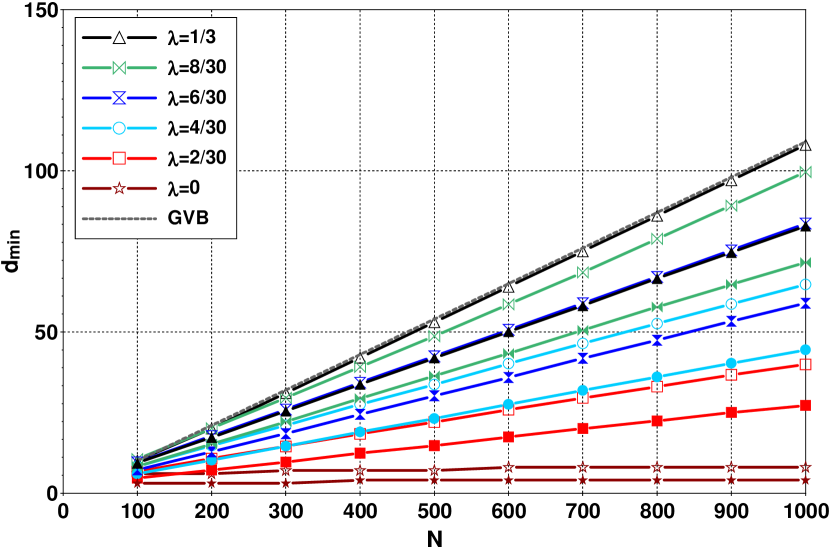
In Fig. 7 we display the same set of curves for the $R=1/2$ type 4 TTCs with 2- and 4-state component encoders. Again, the results are consistent with the asymptotic analysis, and for a given value of the tuning parameter $\lambda$, the minimum distance of the code ensemble with 4-state component encoders is larger than for the code ensemble with 2-state component encoders.

For 4-state RCEs we cannot obtain a closed form WE. However, since 2-state TTCs are asymptotically good, and replacing the accumulators in the outer MPCC with more complex $[5/7]_{8}$ RCEs increases both the asymptotic distance growth rates (see Figs. 3-5) as well as the finite block length minimum distances (see Figs. 6 and 7), we strongly conjecture that the resulting code ensembles with the same structure are still asymptotically good.

V Iterative Decoding Convergence Threshold

To determine the iterative decoding thresholds of tuned turbo code ensembles we employ an extrinsic information transfer (EXIT) chart-based analysis [28]. EXIT charts track the exchange of extrinsic information between component decoders in a concatenated code scheme to estimate its iterative decoding threshold. In the following we briefly describe EXIT charts for type 1 TTCs. The decoder is depicted in Fig. 8. A similar procedure as the one described below can also be applied to type 2, type 3, and type 4 TTCs.

Let $\mathbf{u}_{i}=(u_{0},\ldots,u_{K_{\mathcal{C}_{i}}-1})$ and $\mathbf{x}_{i}=(x_{0},\ldots,x_{N_{\mathcal{C}_{i}}-1})$ be the sequence of information symbols and the sequence of code symbols, respectively, of the $i$th $(N_{{\mathcal{C}}_{i}},K_{{\mathcal{C}}_{i}})$ component code ${\mathcal{C}}_{i}$ of the TTC. (In the following, we will drop the index $i$ when referring to a generic component code.) Each component decoder in Fig. 8 is fed with a priori information (from either other component decoders or the channel) on its information and coded symbols and computes extrinsic information which, in turn, is used by the other component decoders as a priori information. In convergence analysis using EXIT charts it is common to model the a priori information as a Gaussian random variable. Also, as required in EXIT charts analysis, we assume that $K_{{\mathcal{C}}}\rightarrow\infty$ and $N_{{\mathcal{C}}}\rightarrow\infty$. For information symbol $u$ the corresponding a priori L-value (or log-likelihood ratio) is denoted by $L^{\mathcal{C}}_{\mathrm{a}}(u)$. Using the Gaussian approximation, $L^{\mathcal{C}}_{\mathrm{a}}(u)$ can be expressed as:

$$L^{\mathcal{C}}_{\mathrm{a}}(u)=\frac{\sigma_{\mathrm{a},u}^{2}}{2}u+w$$ (32)

where $w$ is a zero-mean Gaussian random variable with variance $\sigma_{\mathrm{a},u}^{2}$. We denote by $I(u;L^{\mathcal{C}}_{\mathrm{a}}(u))$ the mutual information (MI) between $u$ and $L^{\mathcal{C}}_{\mathrm{a}}(u)$. The average a priori MI for the information symbols is

$$\begin{split}I^{\mathcal{C}}_{\mathrm{a},\mathbf{u}}&=\frac{1}{K_{\mathcal{C}}}\sum_{i=0}^{K_{\mathcal{C}}-1}I(u_{i};L^{\mathcal{C}}_{\mathrm{a}}(u_{i})),\end{split}$$ (33)

which depends only on $\sigma_{\mathrm{a},u}$ and can be computed using the $J$ function as $I^{\mathcal{C}}_{\mathrm{a},\mathbf{u}}=J\!\!\left({\sigma_{\mathrm{a},u}}\right)$ [28]. Note that if $u$ is transmitted over the (binary-input Gaussian) channel, $L^{\mathcal{C}}_{\mathrm{a}}(u)$ corresponds to the channel L-value, $L_{\mathrm{ch}(u)}=4R\gamma r$, where $R$ is the code rate, $\gamma$ denotes the SNR $E_{\mathrm{b}}/N_{0}$, $r=\tilde{u}+n$ is the received observation, $\tilde{u}$ is the BPSK modulated symbol, and $n$ is AWGN with variance $N_{0}/2$. In this case it can be easily shown that $\sigma^{2}_{\mathrm{a},u}=8R\gamma$.

For code symbol $x$, the corresponding a priori L-value is denoted by $L^{\mathcal{C}}_{\mathrm{a}}(x)$. Using the Gaussian approximation $L^{\mathcal{C}}_{\mathrm{a}}(x)$ can be written as

$$L^{\mathcal{C}}_{\mathrm{a}}(x)=\frac{\sigma_{\mathrm{a},x}^{2}}{2}x+w,$$ (34)

where $w$ is a zero-mean Gaussian random variable with variance $\sigma^{2}_{\mathrm{a},x}$. As before, we denote by $I(x;L^{\mathcal{C}}_{\mathrm{a}}(x))$ the MI between $x$ and $L^{\mathcal{C}}_{\mathrm{a}}(x)$. The average a priori MI for the code symbols is given by

$$\begin{split}I^{\mathcal{C}}_{\mathrm{a},\mathbf{x}}=\frac{1}{N_{\mathcal{C}}}\sum_{i=0}^{N_{\mathcal{C}}-1}I(x_{i};L^{\mathcal{C}}_{\mathrm{a}}(x_{i})),\end{split}$$ (35)

which can be computed using the $J$ function as $I^{\mathcal{C}}_{\mathrm{a},\mathbf{x}}=J\!\!\left({\sigma_{\mathrm{a},x}}\right)$. If the code symbols are transmitted over the channel, $\sigma^{2}_{\mathrm{a},x}=8R\gamma$.

The a priori L-values $L^{\mathcal{C}}_{\mathrm{a}}(u)$ and $L^{\mathcal{C}}_{\mathrm{a}}(x)$ are inputs to an a posteriori probability (APP) decoder which computes the extrinsic L-values $L^{\mathcal{C}}_{\mathrm{e}}(u)$ and $L^{\mathcal{C}}_{\mathrm{e}}(x)$ for information symbols and code symbols, respectively. The extrinsic L-values are also Gaussian with variance $\sigma^{2}_{\mathrm{e},u}$ and $\sigma^{2}_{\mathrm{e},x}$, respectively. The average extrinsic MI for information and code symbols is given by

$$I^{\mathcal{C}}_{\mathrm{e},\mathbf{u}}=\frac{1}{K_{\mathcal{C}}}\sum_{i=0}^{K_{\mathcal{C}}-1}I(u_{i};L^{\mathcal{C}}_{\mathrm{e}}(u_{i}))$$ (36)

and

$$I^{\mathcal{C}}_{\mathrm{e},\mathbf{x}}=\frac{1}{N_{\mathcal{C}}}\sum_{i=0}^{N_{\mathcal{C}}-1}I(x_{i};L^{\mathcal{C}}_{\mathrm{e}}(x_{i})),$$ (37)

respectively.

The input-output behavior of the APP decoder for encoder ${\mathcal{C}}$ is completely characterized by two EXIT functions, $T_{u}$ and $T_{x}$, which specify the evolution of the extrinsic MIs as a function of the a priori MIs:

$$\begin{split}I^{\mathcal{C}}_{\mathrm{e},\mathbf{u}}&=T_{u}(I^{\mathcal{C}}_{\mathrm{a},\mathbf{u}},I^{\mathcal{C}}_{\mathrm{a},\mathbf{x}})\\ I^{\mathcal{C}}_{\mathrm{e},\mathbf{x}}&=T_{x}(I^{\mathcal{C}}_{\mathrm{a},\mathbf{u}},I^{\mathcal{C}}_{\mathrm{a},\mathbf{x}}).\end{split}$$ (38)

In practice, these functions can be obtained by Monte Carlo simulation for all values $0\leq I^{\mathcal{C}}_{\mathrm{a},\mathbf{u}}\leq 1$ and $0\leq I^{\mathcal{C}}_{\mathrm{a},\mathbf{x}}\leq 1$ by modeling the a priori information as Gaussian distributed, as noted above.

The decoder of the type 1 TTC consists of $q+1$ APP component decoders $\mathcal{C}^{-1}_{1},\ldots,\mathcal{C}^{-1}_{q}$, and $\mathcal{C}^{-1}_{\mathrm{acc}}$ corresponding to the component encoders $\mathcal{C}_{1},\ldots,\mathcal{C}_{q}$ of the outer MPCC and to the inner accumulator, respectively, which iteratively exchange extrinsic information (see Fig. 8). A decoding iteration consists of a single activation of $\mathcal{C}^{-1}_{1},\ldots,\mathcal{C}^{-1}_{q}$ and $\mathcal{C}^{-1}_{\mathrm{acc}}$ in this order. The evolution of the extrinsic MI can then be tracked in a multi-dimensional EXIT chart [29], which plots together the EXIT functions of the $q+1$ component encoders and can be used to predict the convergence threshold. Unfortunately, such a multi-dimensional EXIT chart is hard to visualize. To generate EXIT charts that are easier to deal with, the EXIT functions of the component encoders of the outer MPCC can be combined to obtain the EXIT function of the MPCC, without any precision loss in the prediction of the convergence thresholds [30]. In this way, the behavior of TTCs can be determined by using a two-dimensional EXIT chart, displaying in a single figure the EXIT functions of the outer MPCC and of the inner recursive encoder:

$$\begin{split}I^{\mathcal{C}_{\mathrm{MPCC}}}_{\mathrm{e},\mathbf{x}_{\mathrm{MPCC}}}&=T_{x}(I^{\mathcal{C}_{\mathrm{MPCC}}}_{\mathrm{a},\mathbf{x}_{\mathrm{MPCC}}})\\ I^{\mathcal{C}_{\mathrm{acc}}}_{\mathrm{e},\mathbf{u}_{\mathrm{acc}}}&=T_{u}(I^{\mathcal{C}_{\mathrm{acc}}}_{\mathrm{a},\mathbf{u}_{\mathrm{acc}}},I^{\mathcal{C}_{\mathrm{acc}}}_{\mathrm{a},\mathbf{x}_{\mathrm{acc}}}),\end{split}$$ (39)

where $I^{\mathcal{C}_{\mathrm{MPCC}}}_{\mathrm{a},\mathbf{x}_{\mathrm{MPCC}}}=I^{\mathcal{C}_{\mathrm{acc}}}_{\mathrm{e},\mathbf{u}_{\mathrm{acc}}}$ and $I^{\mathcal{C}_{\mathrm{acc}}}_{\mathrm{a},\mathbf{u}_{\mathrm{acc}}}=I^{\mathcal{C}_{\mathrm{MPCC}}}_{\mathrm{e},\mathbf{x}_{\mathrm{MPCC}}}$. Note that, since the inner accumulator is connected to the channel, $I^{\mathcal{C}_{\mathrm{acc}}}_{\mathrm{a},\mathbf{x}_{\mathrm{acc}}}$ is a function of $\gamma$. In particular, we must distinguish between the MI corresponding to the parity bits generated by the accumulator and the MI corresponding to the input bits, since the two branches are punctured with different puncturing rates. Assuming random puncturing, the a priori MI for the parity bits of the inner accumulator, punctured with rate $\lambda$, is given by $\lambda J(\sqrt{8R\gamma})$, while the a priori MI provided by the channel for the input bits of the inner accumulator, punctured with rate $\mu-\lambda$, is $(\mu-\lambda)J(\sqrt{8R\gamma})$. With these considerations, the EXIT function of the inner accumulator can be written as

$$I^{\mathcal{C}_{\mathrm{acc}}}_{\mathrm{e},\mathbf{u}_{\mathrm{acc}}}=T_{u}(I^{\mathcal{C}_{\mathrm{MPCC}}}_{\mathrm{e},\mathbf{x}_{\mathrm{MPCC}}},(\lambda J(\sqrt{8R\gamma}),(\mu-\lambda)J(\sqrt{8R\gamma}))).$$ (40)

What remains is the computation of $I^{\mathcal{C}_{\mathrm{MPCC}}}_{\mathrm{e},\mathbf{x}_{\mathrm{MPCC}}}$. Looking in more detail at the EXIT functions of the component encoders of the outer MPCC, we observe that the $l$th, $l=\{1,\ldots,4\}$, component decoder is fed with a priori information on $\mathbf{u}_{l}$ generated by all the other component decoders of the MPCC, and with a priori information on $\mathbf{x}_{l}$ provided by the decoder of the inner accumulator. The EXIT functions of the $l$th component of the outer MPCC can then be expressed as

$$\begin{split}I^{\mathcal{C}_{l}}_{\mathrm{e},\mathbf{u}_{l}}&=T^{\mathcal{C}_{l}}_{u}\left(J\left(\sqrt{\sum_{i=1,i\neq l}^{L-1}J^{-1}\left(I^{\mathcal{C}_{i}}_{\mathrm{e},\mathbf{u}_{i}}\right)^{2}}\right),I^{\mathcal{C}_{l}}_{\mathrm{a},\mathbf{x}_{l}}\right)\\ I^{\mathcal{C}_{l}}_{\mathrm{e},\mathbf{x}_{l}}&=T^{\mathcal{C}_{l}}_{x}\left(J\left(\sqrt{\sum_{i=1,i\neq l}^{L-1}J^{-1}\left(I^{\mathcal{C}_{i}}_{\mathrm{e},\mathbf{u}_{i}}\right)^{2}}\right),I^{\mathcal{C}_{l}}_{\mathrm{a},\mathbf{x}_{l}}\right),\end{split}$$ (41)

for information symbols and code symbols, respectively. In (41) we used the fact that $L^{\mathcal{C}_{l}}_{\mathrm{a}}(u)=\sum_{i\neq l}L^{\mathcal{C}_{i}}_{\mathrm{e}}(u)$ and (assuming independence) $\sigma^{2}_{\mathrm{a},u_{l}}=\sum_{i\neq l}\sigma^{2}_{\mathrm{e},u_{i}}$, from which (using the $J$ function) it follows that $I^{\mathcal{C}_{l}}_{\mathrm{a},\mathbf{u}_{l}}=J\left(\sqrt{\sum_{i=1,i\neq l}^{L-1}J^{-1}\left(I^{\mathcal{C}_{i}}_{\mathrm{e},\mathbf{u}_{i}}\right)^{2}}\right)$ [28]. Note that, for the type 1 tuned turbo code, the four EXIT functions $I^{\mathcal{C}_{l}}_{\mathrm{e},\mathbf{u}_{l}}$ and $I^{\mathcal{C}_{l}}_{\mathrm{e},\mathbf{x}_{l}}$ are identical and $I^{\mathcal{C}_{l}}_{\mathrm{a},\mathbf{x}_{l}}=I^{\mathcal{C}_{\mathrm{acc}}}_{\mathrm{e},\mathbf{u}_{\mathrm{acc}}}$.

Figure 8: Decoder for a type 1 TTC.

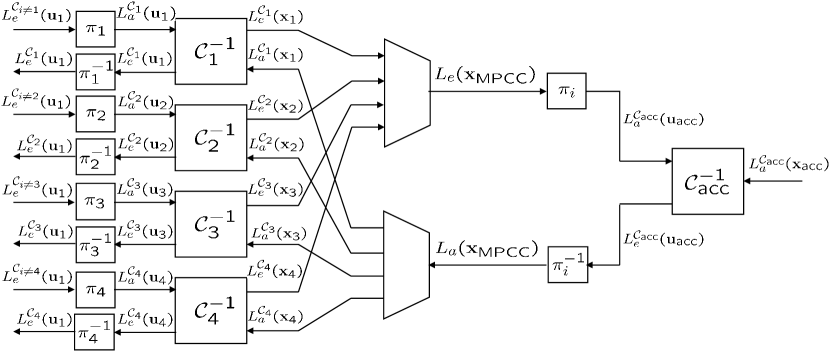
The EXIT function $I^{\mathcal{C}_{\mathrm{MPCC}}}_{\mathrm{e},\mathbf{x}_{\mathrm{MPCC}}}$ can be computed for all values $0\leq I^{\mathcal{C}_{\mathrm{acc}}}_{\mathrm{e},\mathbf{u}_{\mathrm{acc}}}\leq 1$ by activating all $q$ decoders of the MPCC until $I^{\mathcal{C}_{l}}_{\mathrm{e},\mathbf{u}_{l}}$ and $I^{\mathcal{C}_{l}}_{\mathrm{e},\mathbf{x}_{l}}$ have converged to a fixed value. In other words, to obtain the two-dimensional EXIT plot, we assume that a large enough number of iterations is performed within the decoder of the outer MPCC before iterating with the decoder of the inner accumulator. Then, since all component encoders of the outer MPCC are identical, $I^{\mathcal{C}_{\mathrm{MPCC}}}_{\mathrm{e},\mathbf{x}_{\mathrm{MPCC}}}$ is just equal to $I^{\mathcal{C}_{l}}_{\mathrm{e},\mathbf{x}_{l}}$. Finally, the convergence behavior of the type 1 TTC can be tracked by displaying in a single plot the two EXIT functions in (39). The EXIT charts of type 2, type 3, and type 4 TTCs can be computed in a similar way. Note that for type 3 and type 4, the EXIT function of the outer MPCC also depends on $\gamma$ through encoder ${\mathcal{C}}_{0}$, which is directly connected to the channel. For the type 2 TTC, the computation of $I^{\mathcal{C}_{\mathrm{MPCC}}}_{\mathrm{e},\mathbf{x}_{\mathrm{MPCC}}}$ is a bit more complex, since the EXIT function of the first encoder in the outer MPCC is different.

Figure 9: EXIT charts of the type 4 TTC with $\lambda=1$ and $\gamma=1.03$ dB (solid curves with no markers), the type 1 TTC with $\lambda=1$ and $\gamma=2.24$ dB (triangles), and the type 1 TTC with $\lambda=0.3$ and $\gamma=1.09$ dB (circles). $R=1/4$, 2-state component encoders.

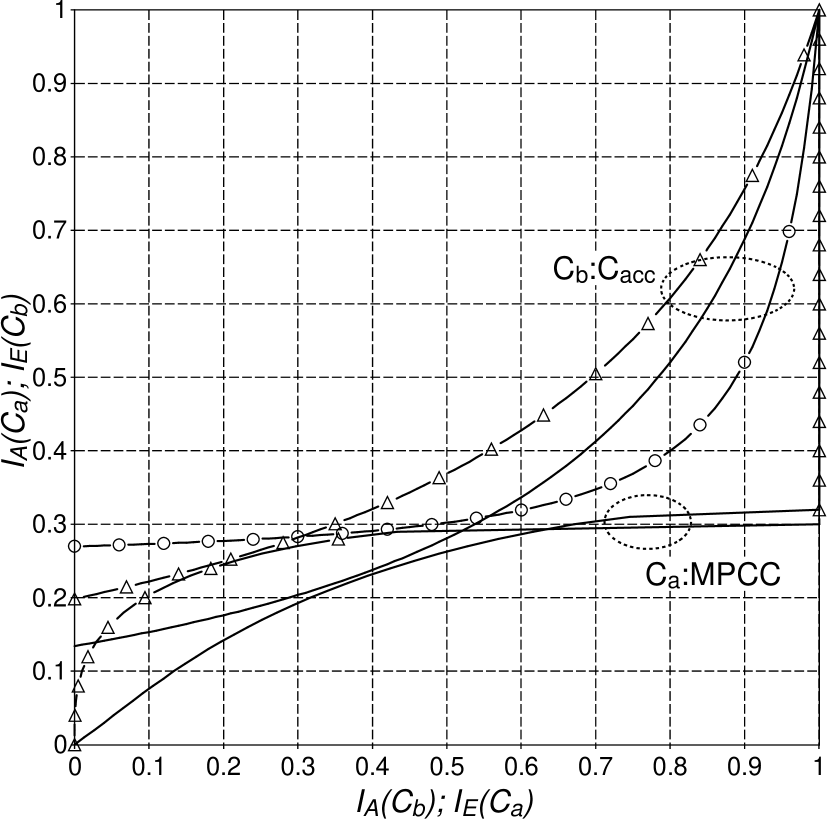
In Fig. 9 we show the EXIT charts of the rate $R=1/4$ type 1 (triangles) and type 4 (solid curves with no markers) TTCs with 2-state component encoders for $\lambda=1$. A vertical step between the lower curves and the upper curves represents a single activation of the inner decoder, while a horizontal step between the upper curves and the lower curves represents an unspecified number of activations of all the component decoders of the MPCC until nothing more can be gained. We observe that the type 4 TTC converges significantly earlier ($\gamma=1.03$ dB) than the type 1 TTC ($\gamma=2.24$ dB), thanks to the systematic branch. Note also that the EXIT chart for the type 1 tuned turbo code is identical to that of the R⁴AA code, where the EXIT function of encoder $\mathcal{C}_{\mathrm{a}}$ in the figure corresponds now to the EXIT function of the repeat-by-four code. The convergence threshold of the type 1 TTC can be significantly improved if some of the parity bits at the output of the inner encoder are replaced by bits from the outer MPCC, at the expense of a smaller asymptotic minimum distance growth rate. For the type 1 TTC with $\lambda=0.3$ (circles) a tunnel opens at $\gamma=1.09$ dB, i.e., $1.15$ dB earlier. In this case, the type 1 TTC with $\lambda=0.3$ has a similar convergence threshold and asymptotic growth rate as the type 4 TTC with $\lambda=1$.

VI Tuning Behavior

In this section we combine the minimum distance results of Section IV and the iterative decoding convergence results from Section V. We observed the tuning effect, namely asymptotic minimum distance growth rates and iterative decoding thresholds increasing with $\lambda$, for all types of tuned turbo codes. However, the effectiveness of tuning depends on the specific combination of distance and threshold results.

Figure 10: Asymptotic minimum distance growth rate $\hat{\rho}$ versus the iterative decoding convergence threshold for the type 4 TTC with 2-state and 4-state encoders in the outer MPCC.

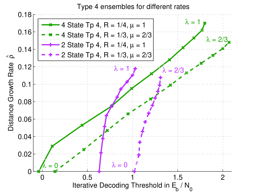
Fig. 10 shows the asymptotic minimum distance growth rate $\hat{\rho}$ versus the iterative decoding convergence threshold for the type 4 TTC with 2-state and 4-state encoders in the outer MPCC, respectively. For all curves, we computed 11 equally spaced values from $\lambda=0$ to $\lambda=\mu$. For $R=1/4$ ($\mu=1$) and $\lambda=1$, the ensemble with 4-state encoders exhibits an asymptotic distance growth rate of $\hat{\rho}=0.17$ and a threshold of $E_{\mathrm{b}}/N_{0}=1.8\,\mathrm{dB}$. Decreasing $\lambda$ leads to better convergence properties, but also to a reduction of the asymptotic distance growth rate. In the extreme case of $\lambda=0$, the code is equal to the outer MPCC consisting of a parallel concatenation of three RCEs and a systematic branch. In this case, the minimum distance does not grow linearly with block length and the asymptotic distance growth rate therefore is zero. Note that the outer MPCC with 4-state encoders has a significantly better iterative decoding convergence threshold ($E_{\mathrm{b}}/N_{0}=-0.04\,\mathrm{dB}$) than the MPCC with 2-state encoders ($E_{\mathrm{b}}/N_{0}=0.63\,\mathrm{dB}$). For $\lambda=1$, the $R=1/4$ 2-state ensemble exhibits a better threshold ($E_{\mathrm{b}}/N_{0}=1.03\,\mathrm{dB}$) but a lower asymptotic distance growth rate ($\hat{\rho}=0.1179$) than the 4-state ensemble. Therefore the dynamic range over which the 2-state ensemble can be adjusted is only 0.4 dB, whereas the 4-state ensemble can be tuned over a larger range of thresholds and asymptotic distance growth rates. This indicates that in the design of TTCs it is important to use an outer MPCC with very good convergence properties.

Puncturing TTCs to rate $R=1/3$ ($\mu=2/3$) results in a right shift of the curves, while leaving their general shape intact. Since the maximum asymptotic distance growth rates (for $\lambda=\mu$) of the underlying $R=1/4$ code ensembles are not very close to the GVB, they are only slightly reduced by the puncturing process (see also Fig. 5).

Figure 11: Gap of the threshold to channel capacity versus the gap of the asymptotic minimum distance growth rate to the GVB for 2-state type 2 and type 3 TTCs and rates $R=1/2$, $1/3$, and $1/4$. As a comparison, for $R=1/2$ the thresholds and asymptotic distance growth rate coefficients of some regular LDPC code ensembles, as well as the ARJA ensemble [23] are also given.

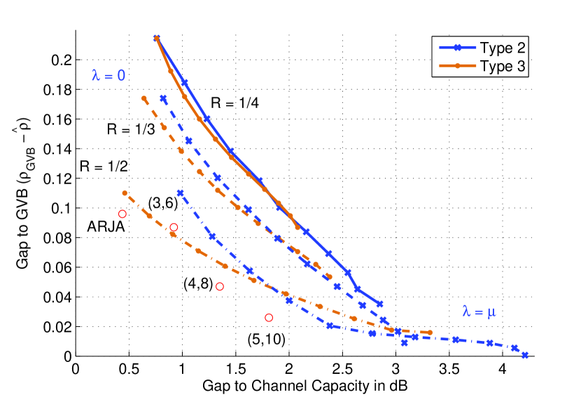
In contrast to Fig. 10, which shows the values for the threshold and the asymptotic distance growth rate directly, in Fig. 11 we show the gap between the convergence threshold and channel capacity and the gap between the asymptotic minimum distance growth rate and the GVB. Since $\hat{\rho}=0$ for $\lambda=0$, the gap of the leftmost point of any curve is equal to the GVB. As $\lambda$ increases, the gap to the GVB decreases, but the gap to channel capacity increases in all cases. For $R=1/4$ and $\lambda=0$, the 2-state type 2 and type 3 ensembles are identical. Due to the FFCE, they exhibit an iterative decoding threshold of $E_{\mathrm{b}}/N_{0}=-0.04\,\mathrm{dB}$, only $0.75\,\mathrm{dB}$ from capacity. For $\lambda>0$, the two ensembles exhibit somewhat different characteristics.

For $\mu=1$ $(R=1/4)$ and $\lambda=1$, the type 2 ensemble has an asymptotic distance growth rate of $\hat{\rho}=0.1793$, corresponding to a gap of $0.0352$ to the GVB, and a threshold of $E_{\mathrm{b}}/N_{0}=2.05\,\mathrm{dB}$, corresponding to a gap to capacity of $2.85\,\mathrm{dB}$, while the type 3 ensemble exhibits a gap to the GVB of $0.0869$ and a gap to capacity of $2.08\,\mathrm{dB}$, which is similar to the type 2 ensemble with $\lambda=0.6$. While puncturing the code ensembles resulted in a right shift of the curves in Fig. 10, in the representation of Fig. 11 puncturing moves the curves closer to the origin, i.e., for a fixed gap to capacity, the gap to the GVB is smaller. It is interesting to note that for $\lambda=0$ the gap to capacity of the type 2 ensemble increases slightly as the rate increases, while for the type 3 ensemble the gap to capacity decreases slightly as the rate increases. The asymptotic distance growth rates for the $R=1/2$ type 2 TTC behave like those shown in Fig. 4 for type 1 ensembles. For small values of $\lambda$ they rapidly increase and then flatten out as the asymptotic distance growth rate approaches the GVB. The iterative decoding threshold, however, continuously increases with $\lambda$, so that the tuning behavior of the $R=1/2$ type 2 ensemble flattens for a stretch before it reaches the GVB at $\lambda=\mu=1/2$. Therefore the parameter range over which the ensemble can be effectively tuned is from $\lambda=0$ to $\lambda=0.2$, which brings the asymptotic distance growth rate to within 0.02 of the GVB.

As a comparison we also give the threshold and asymptotic distance growth rates for rate $R=1/2$ regular LDPC code ensembles and the rate $R=1/2$ ARJA [23] ensemble. With the exemption of the (3,6) LDPC code ensemble, for a given gap to channel capacity, the LDPC code ensembles exhibit a larger asymptotic distance growth rate than the TTC ensembles. However, in contrast to the asymptotically good LDPC codes, TTCs have a simple encoder structure with $O(1)$ encoding complexity. On the other hand, the quasi-cyclic subensemble of the above LDPC codes that also has $O(1)$ encoding complexity is not asymptotically good.

Figure 12: Gap of the threshold to channel capacity versus the relative gap of the asymptotic minimum distance growth rate to the GVB for the 2-state type 3 TTC ensemble with rates $R=1/2$, $1/3$, and $1/4$.

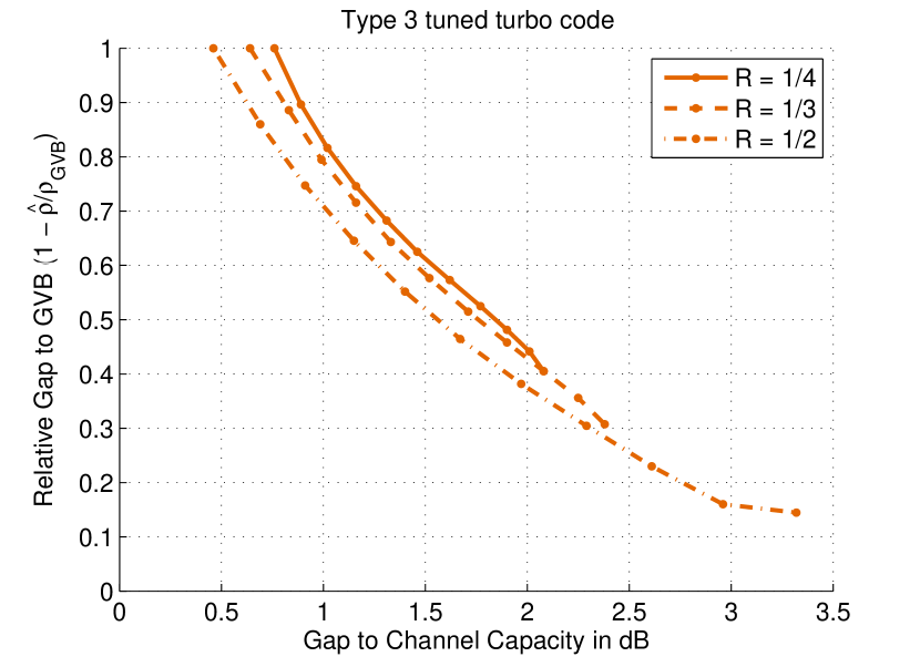
Fig. 12 again shows the tuning behavior of the 2-state type 3 ensemble, but this time the y-axis shows the relative distance from the GVB, namely $1-\frac{\hat{\rho}}{\rho_{GVB}}$. The slopes of the three curves are almost identical. Therefore improving the asymptotic distance growth rate from zero to half of the GVB in each case corresponds to a difference in the convergence threshold of roughly 1 dB. The curves plot the maximum possible range of $\lambda$ values, with $\lambda=0$ corresponding to the topmost point and $\lambda=\mu$ corresponding to the lowest point of each curve.

VII Simulation Results

While the previous sections focused on asymptotic results for the minimum distance and the iterative decoding convergence behavior, in this section we show simulation results illustrating that the tuning principle also applies to relatively short block lengths.

Figure 13: Frame error rate performance of $R=1/4$ ($\mu=1$) type 2 TTCs with 2-state component encoders for different values of the tuning parameter $\lambda$.

We did not make any attempt to optimize the simulated codes but rather focused on the ensemble average code performance. To this end, random interleavers, as well as random puncturing patterns, were employed. Carefully designing the interleavers and puncturing patterns should yield better codes than the ones shown here in terms of error floor performance [31]. Interleaver design, however, usually has little influence on the iterative convergence threshold. The information block length for all simulations is $K=1024$ bits and we use 20 iterations.

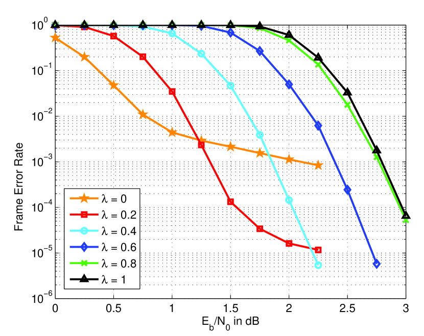
In Fig. 13, we display frame error rate (FER) curves for rate $R=1/4$ type 2 tuned turbo codes with 2-state component encoders and $\lambda\in[0,1]$. The type 2 code with $\lambda=0$ performs best in the waterfall region, but it has a high error floor due to its poor minimum distance. In this case, the code is equivalent to the MPCC in [15]. On the other hand, the code with $\lambda=1$ shows the worst convergence, but according to the analysis in Section IV, it has the best asymptotic minimum distance growth rate, potentially resulting in the lowest error floor. By tuning $\lambda$, we can obtain any behavior in between these two extreme cases: when $\lambda$ decreases, the convergence behavior of the code improves (the curves get closer to the performance of the MPCC), but the error floor is higher. For small values of $\lambda$, where the minimum distance is small, the simulations were able to reach the error floor of the code. Compared to $\lambda=0$, the code with $\lambda=0.2$ loses about 0.5 dB in the waterfall region but the height of the error floor improves by two orders of magnitude. For $\lambda=0.4$, the convergence threshold is again 0.5 dB worse than the $\lambda=0.2$ case, but the error floor is lowered beyond what can be observed in the simulations.

Figure 14: Frame error rate performance of R=1/2 type 4 TTCs with 4-state component encoders for different values of the tuning parameter $\lambda$.

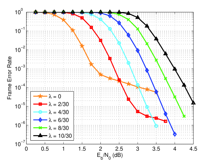
Similar behavior is observed in Fig. 14, where FER curves for rate $R=1/2$ type 4 TTCs with 4-state component encoders are shown. Again, by varying the tuning parameter $\lambda$, we can obtain any behavior between the outer MPCC, which shows the best iterative decoding convergence behavior, and the HCC, which has the best error floor. In particular, the code with $\lambda=0$ performs best in the waterfall region, as predicted by the EXIT charts. However, it has the highest error floor, in agreement with the minimum distance analysis. In general, lower error floors are obtained for increasing values of $\lambda$, but at the expense of poorer performance in the waterfall region. Note that, due to the more powerful 4-state component encoders employed, the error floors of the $R=1/2$ type 4 TTCs are lower than those observed in Fig. 13 for the $R=1/4$ type 2 TTCs with 2-state component encoders.

VIII Conclusions

In this paper, we have introduced a family of hybrid concatenated codes where a tradeoff between asymptotic minimum distance growth rate and iterative decoding threshold can be achieved by varying a tuning parameter $\lambda$. By decreasing $\lambda$, the convergence behavior of the code is improved at the expense of a smaller asymptotic minimum distance growth rate and worse error floor performance, and vice versa. An important advantage of the hybrid tuned turbo code constructions is that they are asymptotically good for a large range of values of $\lambda$, so that even small values of $\lambda$ are sufficient to ensure linear asymptotic distance growth with block length, potentially resulting in low error floors. In addition, a second tuning parameter $\mu$ can be used to change the rate of a TTC ensemble, thereby allowing a system designer to trade off between code rate, iterative decoding convergence behavior, and error floor performance without changing the encoder structure.

Appendix A Proof of Proposition 2

A sequence $\alpha_{i}$, $i=0,1,\ldots,n$, is logarithmically concave if

$$\alpha_{i}^{2}\geq\alpha_{i-1}\cdot\alpha_{i+1}$$

holds for every element $\alpha_{i}$ with $1\leq i\leq n-1$ [32].

1. For the accumulator, we now consider the ratio

   $$R_{w}= \frac{\left(\mathbb{P}^{\mathrm{Acc}(N_{\mathcal{C}})}_{w,h}\right)^{2}}{\mathbb{P}^{\mathrm{Acc}(N_{\mathcal{C}})}_{w,h-1}\mathbb{P}^{\mathrm{Acc}(N_{\mathcal{C}})}_{w,h+1}}$$

   $$= \frac{N_{\mathcal{C}}-h}{N_{\mathcal{C}}-h+1}\cdot\frac{N_{\mathcal{C}}-h-\left\lfloor w/2\right\rfloor+1}{N_{\mathcal{C}}-h-\left\lfloor w/2\right\rfloor}\cdot$$

   $$\frac{h-1}{h}\cdot\frac{h-\left\lceil w/2\right\rceil+1}{h-\left\lceil w/2\right\rceil}.$$

   Since the ratio $\frac{x_{1}}{x_{1}+1}\cdot\frac{x_{2}+1}{x_{2}}>1$ for $x_{1}>x_{2}$, we obtain $R_{1}=1$ for $w=1$ and $R_{w}>1$ for $w>1$. The sequence is thus logarithmically concave. Since the logarithm is a monotonically increasing function, the maximum of the IOWD equals the maximum of the asymptotic IOWD and can thus be obtained by taking the derivative of (12), which is given by

   $$\frac{\partial}{\partial\beta}f^{\mathrm{Acc}}_{\alpha,\beta}=\ln\left(\frac{\beta}{1-\beta}\right)+\ln\left(\frac{1-\beta-\alpha/2}{\beta-\alpha/2}\right),$$ (42)

   so the maximum occurs at $\beta=1/2$, where $f^{\mathrm{Acc}}_{\alpha,1/2}=0$. Correspondingly, the IOWD of the accumulator is maximized for $h=N_{\mathcal{C}}/2$.

2. For simplicity, we consider the terminated 2-state FFCE with even output weight $h$. (Considering the terminated code does not change the asymptotic IOWD of the code.) The ratio $R_{w}$ is given by

   $$R_{w}= \frac{\left(\mathbb{P}^{{\mathrm{FF}}(N_{\mathcal{C}})}_{w,h}\right)^{2}}{\mathbb{P}^{{\mathrm{FF}}(N_{\mathcal{C}})}_{w,h-2}\mathbb{P}^{{\mathrm{FF}}(N_{\mathcal{C}})}_{w,h+2}}$$

   $$= \frac{h/2+1}{h/2-1}\cdot\frac{N_{\mathcal{C}}-w-h/2+1}{N_{\mathcal{C}}-w-h/2-1}\cdot\frac{w-h/2+1}{w-h/2-1}>1.$$

   The sequence is strictly logarithmically concave since every term in the above product is strictly larger than one. The derivative of (13) is given by

   $$\frac{\partial}{\partial\beta}f^{\mathrm{FF}}_{\alpha,\beta}=\frac{1}{2}\ln\left(\frac{\alpha-\beta/2}{\beta/2}\right)+\frac{1}{2}\ln\left(\frac{1-\alpha-\beta/2}{\beta/2}\right),$$ (43)

   so the maximum occurs at $\beta=2\alpha(1-\alpha)$, where $f^{\mathrm{Acc}}_{\alpha,2\alpha(1-\alpha)}=0$. Correspondingly, the IOWD of the 2-state FFCE is maximized for $h=2w(1-w/{N_{\mathcal{C}}})$.

3. For random puncturing, we consider the ratio

   $$R_{h}= \frac{\left(\mathbb{P}^{\mathrm{P}(N^{\prime})}_{h,h^{\prime},\lambda}\right)^{2}}{\mathbb{P}^{\mathrm{P}(N^{\prime})}_{h,h^{\prime}-1,\lambda}\mathbb{P}^{\mathrm{P}(N^{\prime})}_{h,h^{\prime}+1,\lambda}}$$

   $$= \frac{h^{\prime}+1}{h^{\prime}}\cdot\frac{\lambda N-h^{\prime}+1}{\lambda N-h^{\prime}}\cdot$$

   $$\frac{h-h^{\prime}+1}{h-h^{\prime}}\cdot\frac{(1-\lambda)N-h+h^{\prime}+1}{(1-\lambda)N-h+h^{\prime}}>1.$$

   The sequence is strictly logarithmically concave since every term in the above product is strictly larger than one. The derivative of (14) is given by

   $$\frac{\partial}{\partial\beta^{\prime}}f^{\mathrm{P}}_{\beta,\beta^{\prime},\lambda}=-\ln\left(\frac{\beta^{\prime}}{1-\beta^{\prime}}\right)+\ln\left(\frac{\beta-\lambda\beta^{\prime}}{1-\lambda-\beta+\lambda\beta^{\prime}}\right),$$

   so the maximum occurs at $\beta^{\prime}=\beta$, where $f^{\mathrm{P}}_{\beta,\beta,\lambda}=0$. Correspondingly, the IOWD of the random puncturing operation is maximized for $h^{\prime}=\lambda h$.

Appendix B The Total derivative for $F_{1}$

We bound the total derivative of

$$F_{1}=\frac{1}{q}{\mathbb{H}}\left(\alpha\right)+\frac{{\mathcal{I}}_{0}}{q}f^{{\mathcal{C}}_{0}}_{\alpha,\rho_{0}}+\frac{J}{q}f^{\mathrm{Acc}}_{\alpha,\rho_{\mathrm{r}}}+\frac{q-J}{q}f^{\mathrm{FF}}_{\alpha,\rho_{\mathrm{f}}}+f^{\mathrm{Acc}}_{\rho_{\mathrm{p}},\,\rho_{\mathrm{s}}}$$

as $\rho_{\mathrm{p}}\rightarrow 0$.

To capture the dependency of $\rho_{\mathrm{p}}$ on the normalized input weight $\alpha$, the normalized output weight of the 2-state FFCEs $\rho_{\mathrm{f}}$ and the normalized weight of the systematic branch $\rho_{0}$, we parameterize $\alpha$ as $\alpha=a\rho_{\mathrm{r}}$, with $a\in[0,2]$, where the range of $a$ follows from the fact that the output weight of the accumulator cannot be less than half the input weight. Likewise we parameterize $\rho_{\mathrm{f}}=b\alpha=ab\rho_{\mathrm{r}}$, with $b\in[0,2]$. With the above parameterization, the weights $\rho_{\mathrm{p}}$ and $\rho_{\mathrm{r}}$ are related by a multiplicative factor, i.e., $\rho_{\mathrm{p}}=\rho_{\mathrm{r}}(J+ab(q-J))/q$.

We parameterize the output weight of the optional parallel encoder as $\rho_{0}=c\alpha=ac\rho_{\mathrm{r}}$, where $c=0$ if there is no parallel encoder, $c=1$ if there is a simple systematic branch, and $c\in[0,2]$ if the parallel encoder is the 2-state FFCE.

The total derivative w.r.t. $\rho_{\mathrm{p}}$ is then given by

$$\frac{d}{d\rho_{p}} \left.F_{1}\right|_{\begin{subarray}{c}\alpha=a\rho_{\mathrm{r}}\\ \rho_{\mathrm{f}}=ab\rho_{\mathrm{r}}\\ \rho_{0}=ac\rho_{\mathrm{r}}\end{subarray}}=\frac{\partial}{\partial\rho_{\mathrm{p}}}F_{1}+$$

$$\frac{q}{J+ab(q-J)}\left(\frac{\partial}{\partial\rho_{\mathrm{r}}}F_{1}+\frac{\partial}{\partial\alpha}F_{1}\cdot\frac{\partial\alpha}{\partial\rho_{\mathrm{r}}}+\right.$$

$$\left.\left.\frac{\partial}{\partial\rho_{\mathrm{f}}}F_{1}\cdot\frac{\partial\rho_{\mathrm{f}}}{\partial\rho_{\mathrm{r}}}+\frac{\partial}{\partial\rho_{0}}F_{1}\cdot\frac{\partial\rho_{0}}{\partial\rho_{\mathrm{r}}}\right)\right|_{\begin{subarray}{c}\alpha=a\rho_{\mathrm{r}}\\ \rho_{\mathrm{f}}=ab\rho_{\mathrm{r}}\\ \rho_{0}=ac\rho_{\mathrm{r}}\end{subarray}}.$$

The derivatives of the asymptotic IOWDs of the component encoders with respect to their output weight are given by (42) and (43). The derivatives with respect to their input weight are given by

$$\frac{\partial}{\partial\alpha}f^{\mathrm{Acc}}_{\alpha,\beta}= \frac{1}{2}\ln\left(\frac{\beta-\alpha/2}{1-\alpha}\right)+\frac{1}{2}\ln\left(\frac{1-\beta-\alpha/2}{1-\alpha}\right)+\ln 2$$ (44)

$$= \frac{1}{2}\ln\left(4x(1-x)\right),$$

where $x=\frac{\beta-\alpha/2}{1-\beta}$, and

$$\frac{\partial}{\partial\alpha}f^{\mathrm{FF}}_{\alpha,\beta}=2\ln\left(\frac{\alpha}{1-\alpha}\right)+\ln\left(\frac{1-\alpha-\beta/2}{\alpha-\beta/2}\right).$$ (45)

We now evaluate the contributions of the component encoders in $F_{1}$ to the total derivative and show that for $\rho_{\mathrm{p}}\rightarrow 0$, or equivalently $\rho_{\mathrm{r}}\rightarrow 0$, the contribution of each component is either zero or negative. For convenience, for the component encoders of the outer MPCC and the systematic branch we consider the derivative w.r.t $\rho_{\mathrm{r}}$ rather than the derivative w.r.t. $\rho_{\mathrm{p}}$. When the parallel encoder is simply a systematic branch, its contribution to the total derivative is a constant. When the parallel encoder is the 2-state FFCE, its contribution to the total derivative is given by

$$\frac{{\mathcal{I}}_{0}}{q}\frac{\partial}{\partial\alpha} \left.f^{\mathrm{FF}}_{\alpha,\rho_{0}}\right|_{\begin{subarray}{c}\alpha=a\rho_{\mathrm{r}}\\ \rho_{0}=ac\rho_{\mathrm{r}}\end{subarray}}\frac{\partial\alpha}{\partial\rho_{\mathrm{r}}}+\frac{{\mathcal{I}}_{0}}{q}\frac{\partial}{\partial\rho_{0}}\left.{f^{\mathrm{FF}}_{\alpha,\rho_{0}}}\right|_{\begin{subarray}{c}\alpha=a\rho_{\mathrm{r}}\\ \rho_{0}=ac\rho_{\mathrm{r}}\end{subarray}}\frac{\partial\rho_{0}}{\partial\rho_{\mathrm{r}}}$$

$$= \frac{{\mathcal{I}}_{0}a}{q}\left[\ln\left(\frac{1-a\rho_{\mathrm{r}}-ac\rho_{\mathrm{r}}/2}{1-a\rho_{\mathrm{r}}}\right)-\ln\left(1-\frac{c}{2}\right)+\right.$$

$$\left.\ln\left(\frac{a\rho_{\mathrm{r}}}{1-a\rho_{\mathrm{r}}}\right)\right]+\frac{{\mathcal{I}}_{0}ac}{2q}\left[\ln\left(\frac{1-a\rho_{\mathrm{r}}-ac\rho_{\mathrm{r}}/2}{1-a\rho_{\mathrm{r}}}\right)+\right.$$

$$\left.\ln\left(\frac{a\rho_{\mathrm{r}}(1-c/2)}{a\rho_{\mathrm{r}}}\right)-\ln\left(\frac{ac\rho_{\mathrm{r}}/2}{1-a\rho_{\mathrm{r}}}\right)-\ln\left(\frac{ac\rho_{\mathrm{r}}/2}{a\rho_{\mathrm{r}}}\right)\right]$$

$$= \frac{{\mathcal{I}}_{0}a}{q}\left[\underbrace{\ln\left(\frac{(c/2)^{-c/2}(a\rho_{\mathrm{r}})^{1-c/2}}{(1-a\rho_{\mathrm{r}})^{1-c/2}}\right)}_{1}+\right.$$

$$\underbrace{\left(\frac{c}{2}+1\right)\ln\left(\frac{1-a\rho_{\mathrm{r}}(1+c/2)}{1-a\rho_{\mathrm{r}}}\right)}_{2}+$$

$$\left.\underbrace{\left(\frac{c}{2}-1\right)\ln\left(1-\frac{c}{2}\right)}_{3}-\underbrace{\frac{c}{2}\ln\left(\frac{c}{2}\right)}_{4}\right].$$

For $a=0$, the above expression takes on the value zero. For any fixed $a$, $0<a\leq 2$, term 1 is zero for $c=2$ and tends to $-\infty$ otherwise. Term 2 is zero for $c=0$ and strictly negative otherwise, and it vanishes as $\rho_{\mathrm{r}}\rightarrow 0$. Terms 3 and 4 are constants and are zero for $c=0$ and $c=2$.

Similarly, the contribution of the FFCEs in the outer MPCC to the total derivative is given by

$$\frac{q-J}{q}\frac{\partial}{\partial\alpha} \left.f^{\mathrm{FF}}_{\alpha,\rho_{\mathrm{f}}}\right|_{\begin{subarray}{c}\alpha=a\rho_{\mathrm{r}}\\ \rho_{\mathrm{f}}=ab\rho_{\mathrm{r}}\end{subarray}}\frac{\partial\alpha}{\partial\rho_{\mathrm{r}}}+\frac{q-J}{q}\frac{\partial}{\partial\rho_{\mathrm{f}}}\left.{f^{\mathrm{FF}}_{\alpha,\rho_{\mathrm{f}}}}\right|_{\begin{subarray}{c}\alpha=a\rho_{\mathrm{r}}\\ \rho_{\mathrm{f}}=ab\rho_{\mathrm{r}}\end{subarray}}\frac{\partial\rho_{\mathrm{f}}}{\partial\rho_{\mathrm{r}}}$$

$$= \frac{a(q-J)}{q}\left[\ln\left(\frac{(b/2)^{-b/2}(a\rho_{\mathrm{r}})^{1-b/2}}{(1-a\rho_{\mathrm{r}})^{1-b/2}}\right)+\right.$$

$$\left(\frac{b}{2}+1\right)\ln\left(\frac{1-a\rho_{\mathrm{r}}(1+b/2)}{1-a\rho_{\mathrm{r}}}\right)+$$

$$\left.\left(\frac{b}{2}-1\right)\ln\left(1-\frac{b}{2}\right)-\frac{b}{2}\ln\left(\frac{b}{2}\right)\right],$$

and either tends to zero or $-\infty$ as $\rho_{\mathrm{r}}\rightarrow 0$.

The contribution of the RCEs in the outer MPCC to the total derivative is given by

$$\frac{\partial}{\partial\alpha} \left.\left(\frac{1}{q}{\mathbb{H}}\left(\alpha\right)+\frac{J}{q}f^{\mathrm{Acc}}_{\alpha,\rho_{\mathrm{r}}}\right)\right|_{\begin{subarray}{c}\alpha=a\rho_{\mathrm{r}}\end{subarray}}\frac{\partial\alpha}{\partial\rho_{\mathrm{r}}}+\frac{\partial}{\partial\rho_{\mathrm{r}}}\frac{J}{q}\left.{f^{\mathrm{Acc}}_{\alpha,\rho_{\mathrm{r}}}}\right|_{\begin{subarray}{c}\alpha=a\rho_{\mathrm{r}}\end{subarray}}$$

$$= \frac{aJ}{q}\left[-\frac{1}{J}\ln\left(\frac{a\rho_{\mathrm{r}}}{1-a\rho_{\mathrm{r}}}\right)+\frac{1}{2}\ln\left(\frac{\rho_{\mathrm{r}}(1-a/2)}{1-a\rho_{\mathrm{r}}}\right)+\right.$$

$$\left.\frac{1}{2}\ln\left(\frac{1-\rho_{\mathrm{r}}-a\rho_{\mathrm{r}}/2}{1-a\rho_{\mathrm{r}}}\right)+\ln 2\right]+$$

$$\frac{J}{q}\left[\ln\left(\frac{\rho_{\mathrm{r}}}{1-\rho_{\mathrm{r}}}\right)+\ln\left(\frac{1-\rho_{\mathrm{r}}-a\rho_{\mathrm{r}}/2}{\rho_{\mathrm{r}}-a\rho_{\mathrm{r}}/2}\right)\right]$$

$$= \frac{J}{q}\left[\underbrace{\frac{a}{2}\ln\left(\frac{4(a\rho_{\mathrm{r}})^{1-2/J}}{a(1-a\rho_{\mathrm{r}})^{1-2/J}}\right)}_{1}+\underbrace{\frac{a}{2}\ln\left(\frac{1-\rho_{\mathrm{r}}(1+a/2)}{1-a\rho_{\mathrm{r}}}\right)}_{2}+\right.$$

$$\left.\underbrace{\ln\left(\frac{1-\rho_{\mathrm{r}}(1+a/2)}{1-\rho_{\mathrm{r}}}\right)}_{3}+\underbrace{\left(\frac{a}{2}-1\right)\ln\left(1-\frac{a}{2}\right)}_{4}\right].$$

For $a=0$, the above expression is zero. For any fixed $a$, $0<a\leq 2$, and $J>2$, term 1 tends to $-\infty$ as $\rho_{\mathrm{r}}\rightarrow 0$. Terms 2 and 3 vanish for $\rho_{\mathrm{r}}\rightarrow 0$ and term 4 is a constant.

Finally, the contribution of the inner accumulator to the total derivative is given by

$$\frac{\partial}{\partial\rho_{\mathrm{p}}}f^{\mathrm{Acc}}_{\rho_{\mathrm{p}},\rho_{\mathrm{s}}}=\frac{1}{2}\ln\left(4x(1-x)\right),$$ (46)

with $x=\frac{\rho_{\mathrm{s}}-\rho_{\mathrm{p}}/2}{1-\rho_{\mathrm{p}}}$, which is negative for all $x<1/2$, or equivalently $\rho_{\mathrm{s}}<1/2$.

Thus, using $\rho_{s}<\hat{\rho}/(Rq\lambda)$ and the fact that (46) is concave in $x$, for any $0\leq\rho<\hat{\rho}<Rq\lambda/2$, we have

$$\frac{d}{d\rho_{\mathrm{p}}}\left.F_{1}\right|_{\rho_{\mathrm{p}}=0}\leq\frac{1}{2}\ln\left(4\frac{\hat{\rho}}{Rq\lambda}\left(1-\frac{\hat{\rho}}{Rq\lambda}\right)\right)=-C_{2},$$

where we have used the fact that, for $\rho_{\mathrm{p}}\rightarrow 0$, $x\rightarrow\rho_{\mathrm{s}}$.

Christian Koller (S’08) received the B.S. and Dipl.-Ing. degrees in electrical engineering from Technische Universität München, Munich, Germany in 2003 and 2004, respectively. He received the M.S. degree in electrical engineering from University of Notre Dame, Notre dame, IN, in 2008. Since 2005 he is a Research Assistant at the University of Notre Dame, Notre dame, IN, where he is pursuing a Ph.D. in electrical engineering. His research interest include error-correcting codes, network coding, wireless communications, and information theory.

Alexandre Graell i Amat (S’01-M’05-SM’10) was born in Barcelona, Catalonia, Spain, on January 28, 1976. He received the M.Sc. degree in Telecommunications Engineering from the Universitat Politècnica de Catalunya, Barcelona, Catalonia, Spain, in 2001, and the M.Sc. and the Ph.D. degrees in Electrical Engineering from the Politecnico di Torino, Turin, Italy, in 2000 and 2004, respectively. From September 2001 to April 2002, he was a Visiting Scholar at the Center for Magnetic Recording Research, University of California at San Diego, La Jolla, CA. From September 2002 to May 2003, he held a visiting appointment at Universitat Pompeu Fabra, and at the Telecommunications Technological Center of Catalonia, both in Barcelona. During 2001–2004, he also held a part-time appointment at STMicroelectronics Data Storage Division, Milan, Italy, as consultant on coding for magnetic recording channels. From March 2004 to December 2005, he was a Visiting Professor at Universitat Pompeu Fabra. From January 2006 to December 2010 he was with the Department of Electronics of TELECOM Bretagne (former ENST Bretagne), Brest, France. In January 2011 he joined the Department of Signals and Systems at Chalmers University of Technology, Gothenburg, Sweden, where he is currently an Assistant Professor. His research interests are in the areas of Coding and Information Theory. Dr. Graell i Amat is currently an Editor of the IEEE TRANSACTIONS ON COMMUNICATIONS and the IEEE COMMUNICATIONS LETTERS. He is the General Co-Chair of the 7th International Symposium on Turbo Codes & Iterative Information Processing, Gothenburg, Sweden, August 2012. He received the post-doctoral Juan de la Cierva Fellowship of the Spanish Ministry of Education and Science, and the Marie Curie Intra-European Fellowship of the European Commission. He was the runner-up recipient of the IEEE Communications Society “2010 Europe, Middle East & Africa Region Outstanding Young Researcher Award”.

Jörg Kliewer (S’97–M’99–SM’04) received the Dipl.-Ing. (M.Sc.) degree in electrical engineering from Hamburg University of Technology, Hamburg, Germany, in 1993 and the Dr.-Ing. degree (Ph.D.) in electrical engineering from the University of Kiel, Kiel, Germany, in 1999, respectively. From 1993 to 1998, he was a Research Assistant at the University of Kiel, and from 1999 to 2004, he was a Senior Researcher and Lecturer with the same institution. In 2004, he visited the University of Southampton, Southampton, U.K., for one year, and from 2005 until 2007, he was with the University of Notre Dame, Notre Dame, IN, as a Visiting Assistant Professor. In August 2007, he joined New Mexico State University, Las Cruces, NM, as an Assistant Professor. His research interests include network coding, error-correcting codes, wireless communications, and communication networks. Dr. Kliewer was the recipient of a Leverhulme Trust Award and a German Research Foundation Fellowship Award in 2003 and 2004, respectively. He was a Member of the Editorial Board of the EURASIP Journal on Advances in Signal Processing from 2005-2009 and is Associate Editor of the IEEE Transactions on Communications since 2008.

Francesca Vatta received a Laurea in Ingegneria Elettronica in 1992 from University of Trieste, Italy. From 1993 to 1994 she has been with Iachello S.p.A., Olivetti group, Milano, Italy, as system engineer working on design and implementation of Computer Integrated Building (CIB) architectures. Since 1995 she has been with the Department of Electrical Engineering (DEEI) of the University of Trieste where she received her Ph.D. degree in Telecommunications in 1998, with a Ph.D. thesis concerning the study and design of source-matched channel coding schemes for mobile communications. In November 1999 she became assistant professor at the University of Trieste. Starting in 2002, she spent several months as visiting scholar at the University of Notre Dame, Notre Dame, IN, U.S.A., cooperating with the Coding Theory Research Group under the guidance of Prof. D. J. Costello, Jr. Starting in 2005, she spent several months as visiting scholar at the University of Ulm, Germany, cooperating with the Telecommunications and Applied Information Theory Research Group under the guidance of Prof. M. Bossert. She is an author of more than 70 papers published on international journals and conference proceedings. Her current research interests are in the area of channel coding concerning, in particular, the analysis and design of concatenated coding schemes for wireless applications.

Kamil Sh. Zigangirov (M’95 -SM’99 -F’01) was born in the U.S.S.R. in 1938. He received the M.S. degree in 1962 from the Moscow Institute for Physics and Technology,Moscow, U.S.S.R., and the Ph.D. degree in 1966 from the Institute of Radio Engineering and Electronics of the U.S.S.R. Academy of Sciences, Moscow. From 1965 to 1991, he held various research positions with the Institute for Problems of Information Transmission of the U.S.S.R. Academy of Sciences, Moscow, first as a Junior Scientist, and later as a Main Scientist. During this period, he visited several universities in the United States, Sweden, Italy, and Switzerland as a Guest Researcher. He organized several symposia on information theory in the U.S.S.R. In 1994, he received the Chair of Telecommunication Theory at Lund University, Lund, Sweden. From 2003 to 2009, he was a Visiting Professor with the University of Notre Dame, Notre Dame, IN, the Dresden Technical University, Dresden, Germany, and with the University of Alberta, Edmonton, Alberta, Canada. His scientific interests include information theory, coding theory, detection theory, and mathematical statistics. In addition to papers in these areas, he published a book on sequential decoding of convolutional codes (in Russian) in 1974. With R. Johannesson, he coauthored the textbook Fundamentals of Convolutional Coding (IEEE, 1999) and authored Theory of CDMA Communication (IEEE, 2004).

Daniel J. Costello, Jr. (S’62 -M’69 -SM’78 -F’86 -LF’08) was born in Seattle, WA, on August 9, 1942. He received the B.S.E.E. degree from Seattle University, Seattle, WA, in 1964, and the M.S. and Ph.D. degrees in electrical engineering from the University of Notre Dame, Notre Dame, IN, in 1966 and 1969, respectively. He joined the faculty of the Illinois Institute of Technology, Chicago, in 1969 as an Assistant Professor of Electrical Engineering. He was promoted to Associate Professor in 1973, and to Full Professor in 1980. In 1985 he became Professor of Electrical Engineering with the University of Notre Dame, and from 1989 to 1998, served as Chair of the Department of Electrical Engineering. His research interests are in the area of digital communications, with special emphasis on error control coding and coded modulation. He has numerous technical publications in his field, and in 1983 he coauthored a textbook entitled Error Control Coding: Fundamentals and Applications, the 2nd edition of which was published in 2004. Dr. Costello has been a member of the Information Theory Society Board of Governors (BOG) since 1983, and in 1986, he served as President of the BOG. He has also served as Associate Editor for Communication Theory for the IEEE TRANSACTIONS ON COMMUNICATIONS, Associate Editor for Coding Techniques for the IEEE TRANSACTIONS ON INFORMATION THEORY, and Co-Chair of the IEEE International Symposia on Information Theory in Kobe, Japan (1988), Ulm, Germany (1997), and Chicago, IL (2004). In 1991, he was selected as one of 100 Seattle University alumni to receive the Centennial Alumni Award in recognition of alumni who have displayed outstanding service to others, exceptional leadership, or uncommon achievement. In 1999, he received a Humboldt Research Prize from the Alexander von Humboldt Foundation in Germany. In 2000, he was named the Leonard Bettex Professor of Electrical Engineering at the University of Notre Dame. In 2000, he was selected by the IEEE Information Theory Society as a recipient of a Third-Millennium Medal. He was corecipient of the 2009 IEEE Donald G. Fink Prize Paper Award, which recognizes an outstanding survey, review, or tutorial paper in any IEEE publication issued during the previous calendar year.

References

- [1] C. Berrou, A. Glavieux, and P. Thitimajshima, “Near Shannon limit error-correcting coding and decoding: Turbo Codes,” in Proceedings IEEE International Conference on Communications, Geneva, May 1993, pp. 1064–1070.
- [2] D. Divsalar and F. Pollara, “Turbo codes for PCS applications,” Seattle, WA, June 1995.
- [3] N. Kahale and R. Urbanke, “On the minimum distance of parallel and serially concatenated codes,” in Proc. IEEE Int. Symposium on Inform. Theory, Cambridge, MA, Aug. 1998, p. 31.
- [4] M. Breiling, “A logarithmic upper bound on the minimum distance of turbo codes,” IEEE Trans. Inf. Theory, vol. 50, no. 8, pp. 1692–1710, Aug. 2004.
- [5] H. D. Pfister, On the Capacity of Finite State Channels and the Analysis of Convolutional Accumulate-m Codes, Ph.D. Thesis, University of California, San Diego, CA, 2003.
- [6] L. Bazzi, M. Mahdian, and D. A. Spielman, “The minimum distance of turbo-like codes,” IEEE Trans. Inf. Theory, vol. 55, no. 1, pp. 6–15, Jan. 2009.
- [7] F. Fagnani and C. Ravazzi, “Spectra and minimum distances of repeat multiple accumulate codes,” IEEE Trans. Inf. Theory, vol. 55, pp. 4905–4924, Nov. 2009.
- [8] A. Brown, M. Luby, and A. Shokrollahi, “Repeat-accumulate codes that approach the Gilbert-Varshamov bound,” in Proc. IEEE Int. Symposium on Inform. Theory, Adelaide, Australia, Sept. 2005, pp. 169–173.
- [9] D. Divsalar and F. Pollara, “Serial and hybrid concatenated codes with applications,” in Proc. Int. Symp. on Turbo Codes & Related Topics, Brest, France, Sept. 1997, pp. 80–87.
- [10] C. Koller, A. Graell i Amat, J. Kliewer, F. Vatta, and D. J. Costello, Jr., “Hybrid concatenated codes with asymptotically good distance growth,” in Proc. Int. Symp. on Turbo Codes & Related Topics, Lausanne, Switzerland, Sept. 2008.
- [11] A. Graell i Amat and E. Rosnes, “Good concatenated code ensembles for the binary erasure channel,” IEEE J. Sel. Areas in Commun., vol. 27, no. 6, pp. 928–943, July 2009.
- [12] C. Koller, A. Graell i Amat, J. Kliewer, F. Vatta, and D. J. Costello, Jr., “Tuned turbo codes,” in Proc. Int. Symposium on Inform. Theory and its Applications, Auckland, New Zealand, Dec. 2008.
- [13] E. Rosnes and A. Graell i Amat, “Performance analysis of 3-D turbo codes,” IEEE Trans. Inf. Theory, vol. 57, no. 6, pp. 3707–3720, May 2011.
- [14] R. Smarandache and P. O. Vontobel, “Quasi-cyclic LDPC codes: influence of proto- and Tanner-graph structure on minimum Hamming distance upper bounds,” IEEE Trans. Inf. Theory, vol. 58, no. 2, pp. 585–607, Feb. 2012.
- [15] P. C. Massey and D. J. Costello, Jr., “New low-complexity turbo-like codes,” in Proc. IEEE Information Theory Workshop, Cairns, Australia, Sept. 2001.
- [16] C. He, A. Banerjee, D. J. Costello, Jr., and P. C. Massey, “On the performance of low complexity multiple turbo codes,” in Proc. 40th Annual Allerton Conf. Commun., Control, Computing, Monticello, IL, Sept. 2002.
- [17] C. Koller, A. Graell i Amat, J. Kliewer, and D. J. Costello, Jr., “Trapping set enumerators for repeat multiple accumulate code ensembles,” in Proc. IEEE Int. Symposium on Inform. Theory, Seoul, Korea, June 2009, pp. 1819–1823.
- [18] F. R. Kschischang, B. J. Frey, and H.-A. Loeliger, “Factor graphs and the sum-product algorithm,” IEEE Trans. Inf. Theory, vol. 47, pp. 498–519, Feb. 2001.
- [19] P. O. Vontobel and R. Koetter, “Graph-cover decoding and finite-length analysis of message-passing iterative decoding of LDPC codes,” CoRR, http://www.arxiv.org/abs/cs.IT/0512078, Dec. 2005.
- [20] J. Feldman, T. Malkin, R. A. Servedio, C. Stein, and M. J. Wainwright, “LP decoding corrects a constant fraction of errors,” IEEE Trans. Inf. Theory, vol. 53, pp. 82–89, Jan. 2007.
- [21] S. Benedetto, D. Divsalar, G. Montorsi, and F. Pollara, “Analysis, design, and iterative decoding of double serially concatenated codes with interleavers,” IEEE J. Sel. Areas in Commun., vol. 16, no. 2, pp. 231–244, Feb. 1998.
- [22] D. Divsalar, H. Jin, and R. J. McEliece, “Coding theorems for ‘turbo-like’ codes,” in Proc. 36th Annual Allerton Conf. Commun., Control, Computing, Monticello, IL, Sept. 1998, pp. 201–210.
- [23] A. Abbasfar, D. Divsalar, and K. Yao, “Accumulate-repeat-accumulate codes,” IEEE Trans. Comm., vol. 55, pp. 692–702, Apr. 2007.
- [24] R. G. Gallager, Low-Density Parity-Check Codes, MIT Press, Cambridge, MA, 1963.
- [25] H. Jin and R. J. McEliece, “Coding theorems for turbo code ensembles,” IEEE Trans. Inf. Theory, vol. 48, no. 6, pp. 1451–1461, June 2002.
- [26] C. T. Kelley, Iterative Methods for Optimization, Society for Industrial and Applied Mathematics, Philadelphia, PA, 1999.
- [27] I. Sason, E. Telatar, and R. Urbanke, “The asymptotic input output weight distribution of convolutional codes,” IEEE Trans. Inf. Theory, vol. 48, no. 12, pp. 3052–3061, Dec. 2002.
- [28] S. ten Brink, “Convergence behavior of iteratively decoded parallel concatenated codes,” IEEE Trans. Comm., vol. 49, no. 2, pp. 1727–1737, Oct. 2001.
- [29] M. Tüchler, “Convergence prediction for iterative decoding of threefold concatenated systems,” in Proc. IEEE Global Telecommun. Conf., Taipei, Taiwan, Nov. 2002, pp. 1358–1362.
- [30] F. Brännström, L. K. Rasmussen, and A. J. Grant, “Convergence analysis and optimal scheduling for multiple concatenated codes,” IEEE Trans. Inf. Theory, vol. 51, no. 9, pp. 3354–3364, Sept. 2005.
- [31] C. He, M. Lentmaier, D. J. Costello, Jr., and K. S. Zigangirov, “Joint permutor analysis and design for multiple turbo codes,” IEEE Trans. Inf. Theory, vol. 52, no. 9, pp. 4068–4083, Sept. 2006.
- [32] R. P. Stanley, “Log-concave and unimodal sequences in algebra, combinatorics, and geometry,” Graph Theory and Its Applications: East and West, Ann. New York Acad. Sci., vol. 576, pp. 500–535, 1989.