Good, great, or lucky? Screening for firms with sustained superior performance using heavy-tailed priors

Abstract

This paper examines historical patterns of ROA (return on assets) for a cohort of 53,038 publicly traded firms across 93 countries, measured over the past 45 years. Our goal is to screen for firms whose ROA trajectories suggest that they have systematically outperformed their peer groups over time. Such a project faces at least three statistical difficulties: adjustment for relevant covariates, massive multiplicity, and longitudinal dependence. We conclude that, once these difficulties are taken into account, demonstrably superior performance appears to be quite rare. We compare our findings with other recent management studies on the same subject, and with the popular literature on corporate success.

Our methodological contribution is to propose a new class of priors for use in large-scale simultaneous testing. These priors are based on the hypergeometric inverted-beta family, and have two main attractive features: heavy tails and computational tractability. The family is a four-parameter generalization of the normal/inverted-beta prior, and is the natural conjugate prior for shrinkage coefficients in a hierarchical normal model. Our results emphasize the usefulness of these heavy-tailed priors in large multiple-testing problems, as they have a mild rate of tail decay in the marginal likelihood $m(y)$—a property long recognized to be important in testing.

and

1 Introduction

1.1 Large-scale screening of historical ROA data

Understanding the reasons why some firms thrive and others fail is one of the primary goals of research in strategic management. Studies that examine successful companies to uncover the putative secrets of successful companies are very popular, both in the academic and popular literature.

Before the search for special causes can begin, however, success must be quantified and benchmarked. This is what our paper tries to do. In keeping with prior studies [McGahan and Porter (1999), Wiggins and Ruefli (2005), Henderson, Raynor and Ahmed (2009)], we use a common metric called ROA, or return on assets, to measure a company’s success. This quantity gives investors some notion of how effectively a firm uses its available funds to produce income. It is fundamentally different from a market-based measure like stock returns, which may fail to reflect underlying fundamentals over long periods of time (e.g., during bubbles), and which exhibit wild fluctuations that make the identification of trends problematic. Figure 1 shows three examples of firm-level ROA trajectories over time; these have been standardized using a procedure which we will soon describe.

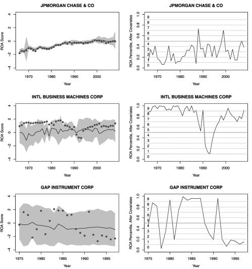
Figure 1: Left: the actual performance of three firms (dots), superimposed on the benchmark distribution estimated from the Bayesian regression-tree model (black line and grey area, showing the posterior mean and $95\%$ predictive interval of expected performance by all firms in the corresponding peer group). Right: these same firms placed on a common (normal CDF) scale of benchmarked performance, with the integers 0–9 representing the decile.

In this paper we apply Bayesian methods to historical ROA data, with the goal of comparing publicly traded companies against their peers. To be sure, ROA is an imperfect measure of corporate success, and our study will have the same shortcomings in this regard as any other that uses ROA as an outcome variable. One important practical reason for our use of ROA, aside from a desire to use the same metric as other researchers studying similar questions, is the sheer availability of data on companies from across the world (rather than just in the United States). This enables us to screen as large a database as possible: 645,456 records from 53,038 companies in 93 different countries, spanning 1966–2008. In principle, however, our Bayesian statistical methodology could be applied to any outcome variable in any subpopulation of the corporate universe.

We conclude that evidence of sustained superior performance is quite rare. To reach this conclusion, we use Bayesian models to compute the posterior probability that a firm falls into each of two classes: a null class, wherein deviations from the peer-group average are attributable to chance; and an alternative class, wherein these deviations, both positive and negative, are systematic. These posterior probabilities depend upon the particular assumptions made about the longitudinal persistence of “lucky” performances, in a manner soon to be explained. But even under the generous (and unrealistic) assumption of longitudinal independence, we find that there are at most 1076 firms over the last 45 years for which there is moderately strong evidence of sustained superior performance over 5 years or more. We argue that this is a conservative upper bound on the number of such firms, and that the actual number is much smaller—our best estimate is 262, or $0.5\%$ of all firms, once longitudinal dependence is taken into account.

1.2 Statistical issues in identifying sustained superior performance

Any attempt to benchmark performance, and to identify sustained superior performers, must deal with at least three statistical challenges.

First, one must adjust observed performance for relevant covariates. One important covariate is a firm’s country of operation. Another one is a firm’s industry; as Henderson, Raynor and Ahmed (2009) observe, some industries exhibit structures that are intrinsically more favorable to monopolies, which would seem to be a source of advantage unrelated to managerial talent or firm-level characteristics. Other potentially important characteristics that have been explored in the literature include a firm’s size and capital structure.

Our method adjusts for the effect of all of these covariates, both on the conditional mean and conditional variance of performance. Importantly, there is no reason to assume that ROA depends upon them linearly. This is quite different from the situation in finance, for example, where the capital-asset pricing model (CAPM) and its variants predict a linear dependence between firm-level and market-level measures of performance. No such theory exists that would predict a parallel result for ROA. This means that nonlinear relationships must, at least in principle, be allowed. We do this using Bayesian treed-regression models, as described in Section 4.

Second, even “lucky” performance trajectories may exhibit significant longitudinal dependencies that lead to spurious declarations of impressiveness. Following Denrell (2005), imagine a very simple state-space model, wherein

$$y_{t} = ax_{t}+e_{t},$$

$$x_{t} = bx_{t-1}+u_{t},$$

where $y_{t}$ is an observed performance metric, and $x_{t}$ is some underlying AR(1) firm-level characteristic (e.g., resources). Even if there is no systematic component of variation in $x_{t}$, the observed $y_{t}$’s can still exhibit pronounced longitudinal autocorrelation, which can look very much like a sustained run of excellence. Formally correcting for such autocorrelation would require specific parametric models incorporating a wide variety of firm-level effects. Instead of taking this route, we try to correct for longitudinal dependence in a crude-but-simple fashion by estimating an effective sample size for each firm, and adjusting our Bayesian model accordingly.

Finally, there is the issue of massive multiplicity. Given the large number of hypothesis tests being conducted, and the frequentist leanings of the management-theory community, maintaining control over false positives is crucial. Yet having access to the posterior distribution of effect sizes can greatly inform follow-up case studies of individual firms, and is only possible under a fully Bayesian model. This applied context makes a combined Bayes/frequentist approach especially appealing.

Our paper’s methodological innovation is to introduce a new class of heavy-tailed priors for the multiple-testing problem. We first give a brief overview of this problem from a Bayesian perspective (Section 2), deferring much of the details to Appendices. We then describe some simulation studies in Section 3, which are designed to benchmark our proposed method against reasonable alternatives. In these studies, our methods show excellent performance in terms of limiting false positives, lending credence to the results for the actual data. Finally, we analyze the corporate ROA data in Section 4, where we also describe in further detail how we approach the other statistical issues we have raised.

2 Large-scale simultaneous testing

2.1 Methodological overview

In large-scale simultaneous testing, thegoal is to uncover lower-dimensional signals from high-dimensional data. For example, researchers who use microarrays have long been interested in the problem of multiplicity adjustment, where “adjustment” can be understood in the sense of adjusting one’s tolerance for surprise as the set of potentially surprising events grows large. The same issue arises in all modern high-throughput experiments; other examples include functional magnetic-resonance imaging, environmental sensor networks, combinatorial chemistry, and proteomics. Too many type-I errors will mean too many expensive wild-goose chases. Hence, the case for a testing procedure that displays good frequentist properties is very compelling.

But so too is the case for a model-based Bayesian procedure. These experiments may involve thousands of separate tests, and such a large volume of data often allows the distributional properties of “signals” and “noise” to be characterized quite precisely.

This paper considers a new version of the two-groups multiple-testing model, where we observe data $y_{i}$ for $i=(1,\ldots,p)$ according to a hierarchical model:

$$(y_{i}\mid\beta_{i},\sigma^{2}) \sim \mathrm{N}(\beta_{i},\sigma^{2}),$$

$$(\beta_{i}\mid w,\theta) \sim w\cdot g(\beta_{i}\mid\theta)+(1-w)\cdot\delta_{0},$$

$$w \sim p(w),$$

a mixture of a Dirac measure at zero, and an alternative model $g$ that is absolutely continuous with respect to the Lebesgue measure. (The alternative model $g$ has hyperparameter $\theta$, presumably also given a prior.) The most attractive feature of this model is that it automatically adjusts for multiplicity, without the need for ad-hoc regularization. This is because inference for the $\beta_{i}$’s will involve the posterior for common mixing fraction, $p(w\mid\mathbf{y})$. If one tests many noise observations in the presence of a few signals, then our estimate of $w$ will be small, making it more difficult for all the observations to overcome the prior belief in their irrelevance. This exerts a powerful form of control over false positives.

To handle the multiple-testing problem, we introduce a family of distributions $g$ based on normal variance mixtures, where the mixing distribution is a hypergeometric inverted-beta (HIB) prior:

$$(\beta_{i}\mid\lambda_{i}^{2},\gamma_{i}=1) \sim \mathrm{N}(0,\sigma^{2}\lambda_{i}^{2}),$$

$$\lambda_{i}^{2} \sim \operatorname{HIB}(a,b,\tau,s),$$

where the indicator $\gamma_{i}=1$ if $\beta_{i}$ is nonzero, and zero otherwise. We approach these priors from a hybrid Bayesian/frequentist perspective, using them to compute not only posterior distributions, but also false-discovery rates, or FDR [Benjamini and Hochberg (1995)]. We also study the behavior of the posterior mean, which is competitive with existing gold-standard methods [e.g., Johnstone and Silverman (2004)] under squared-error loss.

In both our data analysis and simulation studies, we focus on three key features of our approach: [(1)]

The hypergeometric inverted-beta scale mixtures form an especially flexible class of symmetric, unimodal densities and can accommodate a wide range of tail behavior and behavior near the centering parameter. This class simultaneously generalizes the robust priors of Strawderman (1971) and Berger (1980), the normal-exponential-gamma prior of Griffin and Brown (2005), and the horseshoe prior of Carvalho, Polson and Scott (2010). The ability of our class to model heavy-tailed distributions with minimal computational fuss is of particular relevance in testing problems [see, e.g., Section 5.2 of Jeffreys (1961)].

Our class of priors allows very easy computation of a wide array of important Bayesian and frequentist quantities. This includes posterior means, variances, and higher-order moments; posterior null probabilities for individual observations; the score function; false-discovery rates; and local false-discovery rates [Efron (2008)]. The ease with which these quantities can be computed all relates to the analytical tractability of the marginal likelihood function $m(y)$, whose importance we describe in Section 2.2. Appendix A provides all the details.

Our approach yields testing error rates that are competitive with existing cutting-edge methods. At the same time, it also retains the advantages of a fully Bayesian procedure, in that in principle one has access to the joint posterior distribution of all parameters.

Many of the technical details characterizing the behavior of the basic mixture model can be found in Scott and Berger (2006) and Bogdan, Chakrabarti and Ghosh (2008). These authors assume that the nonzero means follow a normal distribution, an assumption we generalize in this paper. Do, Müller and Tang (2005) also provide an interesting variation wherein the nonzero means are modeled nonparametrically using Dirichlet processes.

The same issues arise in empirical-Bayes analysis. See, for example, Johnstone and Silverman (2004), Abramovich et al. (2006) and Dahl and Newton (2007). Additionally, Müller, Parmigiani and Rice (2007), Bogdan, Ghosh and Tokdar (2008) and Park and Ghosh (2010). All describe the relationship between Bayesian multiple testing and classical approaches that control the false-discovery rate.

2.2 The importance of the marginal likelihood function

Many common Bayesian and frequentist treatments of the multiple-testing problem can be understood through the marginal likelihood functions

$$m_{0}(y\mid\sigma^{2}) = \mathrm{N}(y\mid 0,\sigma^{2}),$$

$$m_{1}(y\mid\theta) = \int_{\mathbb{R}}\mathrm{N}(y_{i}\mid\beta_{i},\sigma^{2})g(\beta_{i}\mid\theta)\,\mathrm{d}\beta_{i},$$

$$m(y\mid\theta,\sigma^{2}) = w\cdot m_{1}(y)+(1-w)\cdot m_{0}(y).$$

First, following Efron (2008), the local FDR and the posterior probability of $y_{i}$ being noise are given by the same expression:

$$fdr(y)=P(\beta_{i}=0\mid y,\sigma^{2},\theta)=\frac{(1-w)\cdot m_{0}(y)}{m(y)}.$$

Furthermore, if we let $F_{0}(y)=\int_{-\infty}^{y}m_{0}(u)\,\mathrm{d}u$, $F_{1}(y)=\int_{-\infty}^{y}m_{1}(u)\,\mathrm{d}u$, and $F(y)=w\cdot F_{1}(y)+(1-w)\cdot F_{0}(y)$, then the FDR is the tail area

$$\operatorname{FDR}(y)=\frac{(1-w)\cdot F_{0}(y)}{F(y)}.$$

Second, the marginal likelihood function also arises in Masreliez’s classic representation of the posterior mean. This gives an explicit expression for the Bayes estimator for $\beta_{i}$ under squared-error loss (assuming that $\gamma_{i}=1$):

$$\mathrm{E}(\beta_{i}\mid y,\gamma_{i}=1)=y_{i}+\frac{d}{dy_{i}}\ln m_{1}(y_{i}),$$

versions of which appear in Masreliez (1975), Polson (1991), Pericchi and Smith (1992) and Carvalho, Polson and Scott (2010). The choice of alternative model $g(\beta_{i}\mid\theta)$ is crucial, insofar as it helps to determine $m_{1}(y)$.

At the same time, the prior should have desirable statistical properties, with flat tails being a particularly important feature. The use of heavy-tailed priors for constructing robust shrinkage estimators has a long history, with prominent examples to be found in Strawderman (1971) and Berger (1980). Jeffreys, meanwhile, observed as early as 1939 that heavy-tailed priors play an important role in Bayesian hypothesis testing [see Jeffreys (1961), a later edition]. His arguments have been recapitulated in the context of linear models by Zellner and Siow (1980) and, more recently, Liang et al. (2008).

The difficulty is that, while heavy-tailed priors lead to a desirably mild rate of tail decay in the marginal likelihood $m(\mathbf{y})$, there are few such priors that are also analytically tractable. Any prior that possesses both properties, as our proposed family does under certain hyperparameter choices, is therefore of great potential interest to Bayesians and non-Bayesians alike.

We describe the hypergeometric-beta family of priors more fully in a lengthy technical Appendix. But first we present simulation studies that demonstrate the usefulness of our approach for limiting false positives, before turning to an analysis of the data set at hand.

3 Simulation studies

As our methodological Appendix shows, hypergeometric inverted-beta scale mixtures of normals are an especially useful class of priors for building discrete mixture models for $\beta_{i}$, due to the existence of simple expressions for moments and marginals under the hypothesis that $\beta_{i}$ is nonzero:

$$(\beta_{i}\mid\kappa_{i}) \sim w\cdot\mathrm{N}(0,\kappa^{-1}-1)+(1-w)\cdot\delta_{0},$$ (1)

$$\kappa_{i} \sim \operatorname{HB}(a,b,\tau,s),$$ (2)

where $\delta_{0}$ indicates a degenerate distribution at 0. The posterior mean under this model is a natural estimator for $\bolds{\beta}=(\beta_{1},\ldots,\beta_{p})$, since it averages over uncertainty about whether each component is zero or nonzero.

We conducted two simulation studies comparing the mean-squared error performance of our estimators with the procedure from Johnstone and Silverman (2004), where $\beta_{i}$ is estimated by the posterior median under a mixture of a point mass zero and a double-exponential (Laplace) prior. We also keep track of the number of false positives generated by each procedure.

Each of the two studies involved estimating signals from a different signal class. In all cases the dimension of the location vector was $p=1\mbox{,}000$.

Table 1 summarizes an experiment involving 12

Table 1: Experiment 1, fixed coefficients. SSE: sum of squared errors in the estimate of the $\bolds{\beta}$ sequence. FP: false positive declarations in the estimate of $\bolds{\beta}$ sequence. FDR: realized false-discovery rate. Laplace: posterior median estimator from the empirical Bayes procedure of Johnstone and Silverman (2004). The numbers in parentheses indicate, in order, the choices of $a$ and $b$ the HIB model

		Number nonzero out of 1,000 means
		5				50				100
Value:		3	4	5	7	3	4	5	7	3	4	5	7
SSE	Laplace	$35.1$	$32.8$	$17.9$	$8.5$	$210.5$	$150.8$	$99.7$	$71.9$	$331.1$	$248.3$	$177.5$	$142.9$
	$(1,2)$	$35.4$	$31.9$	$17.9$	$10.3$	$205.4$	$157.7$	$116.7$	$90.6$	$334.6$	$268.2$	$213.2$	$180.4$
	$(1,1)$	$35.0$	$31.3$	$18.5$	$11.1$	$200.5$	$161.9$	$124.7$	$95.3$	$329.1$	$280.8$	$229.3$	$188.5$
	$(1,0.5)$	$34.7$	$31.0$	$19.6$	$12.2$	$199.6$	$170.7$	$135.3$	$100.6$	$335.2$	$302.2$	$248.1$	$196.3$
	$(0.5,2)$	$37.9$	$36.8$	$18.3$	$7.3$	$242.6$	$167.3$	$104.0$	$70.8$	$395.3$	$272.8$	$182.8$	$145.7$
	$(0.5,1)$	$37.6$	$36.3$	$18.1$	$7.6$	$234.9$	$164.1$	$105.0$	$72.6$	$379.5$	$268.8$	$186.4$	$148.9$
	$(0.5,0.5)$	$37.4$	$35.7$	$17.9$	$7.9$	$227.5$	$161.1$	$106.2$	$74.2$	$363.6$	$266.2$	$190.9$	$151.9$
FP	Laplace	$0.8$	$1.0$	$0.8$	$0.4$	$16.1$	$11.3$	$7.6$	$4.2$	$53.3$	$28.7$	$17$	$8.9$
	$(1,2)$	$0.2$	$0.3$	$0.6$	$0.5$	$4.0$	$6.9$	$6.6$	$5.5$	$12.2$	$18.2$	$17.2$	$13.2$
	$(1,1)$	$0.2$	$0.4$	$0.7$	$0.5$	$6.4$	$10.2$	$9.4$	$6.9$	$23.7$	$34.0$	$29.2$	$18.7$
	$(1,0.5)$	$0.3$	$0.6$	$0.8$	$0.7$	$13.5$	$21.1$	$16.9$	$9.8$	$153.5$	$199.8$	$90.0$	$33.4$
	$(0.5,2)$	$0.1$	$0.1$	$0.1$	$0.2$	$1.1$	$2.5$	$2.2$	$2.2$	$2.9$	$5.5$	$5.4$	$5.1$
	$(0.5,1)$	$0.1$	$0.1$	$0.2$	$0.2$	$1.4$	$3.0$	$2.7$	$2.5$	$3.7$	$7.1$	$6.7$	$5.9$
	$(0.5,0.5)$	$0.1$	$0.1$	$0.2$	$0.2$	$1.7$	$3.7$	$3.1$	$2.8$	$5.5$	$9.5$	$8.6$	$6.8$
FDR	Laplace	$0.2$	$0.2$	$0.1$	$0.1$	$0.3$	$0.2$	$0.1$	$0.1$	$0.4$	$0.2$	$0.1$	$0.1$
	$(1,2)$	$0.1$	$0.1$	$0.1$	$0.1$	$0.1$	$0.1$	$0.1$	$0.1$	$0.1$	$0.2$	$0.1$	$0.1$
	$(1,1)$	$0.1$	$0.1$	$0.1$	$0.1$	$0.2$	$0.2$	$0.2$	$0.1$	$0.2$	$0.3$	$0.2$	$0.2$
	$(1,.5)$	$0.2$	$0.1$	$0.1$	$0.1$	$0.3$	$0.3$	$0.2$	$0.2$	$0.6$	$0.6$	$0.5$	$0.2$
	$(0.5,2)$	$0.1$	$0.0$	$0.0$	$0.0$	$0.0$	$0.1$	$0.0$	$0.0$	$0.1$	$0.1$	$0.1$	$0.0$
	$(0.5,1)$	$0.1$	$0.0$	$0.0$	$0.0$	$0.1$	$0.1$	$0.1$	$0.0$	$0.1$	$0.1$	$0.1$	$0.1$
	$(0.5,0.5)$	$0.1$	$0.0$	$0.0$	$0.0$	$0.1$	$0.1$	$0.1$	$0.1$	$0.1$	$0.1$	$0.1$	$0.1$

configurations of different sparsity patterns (5, 50, and 100 nonzero means) and different scales (all nonzero means equal to 3, 4, 5, or 7).

Table 2 summarizes an experiment in which the nonzero means were randomly drawn from a heavy-tailed $t$ distribution with 5 degrees of freedom and scale parameter $c$. We investigated 12 configurations of different sparsity patterns (20, 50, 200, and 500 nonzero means) and different scales ($c=0.5,1,2$).

Tables 1 and 2 show the average sum of squared errors in estimating $\bolds{\beta}$ over 100 independent data sets. Also shown are the average number of false positives declared by the two procedures in each case, and the average false-discovery rate. For the Johnstone/Silverman procedure, a false positive occurs when the posterior median of $\beta_{i}$ is nonzero, but the actual value is zero. For the Bayesian procedure using the hypergeometric inverted-beta prior, a false positive occurs when the posterior inclusion probability for $\beta_{i}$ is greater than $50\%$ and $\beta_{i}$ is actually zero. This threshold reflects a 0–1 loss function that penalizes false positives and false negatives equally, regardless of size. A full decision-theoretic analysis incorporating more realistic loss functions would yield a different, data-adaptive threshold, but would only complicate the analysis slightly.

For the hypergeometric inverted-beta prior, we set $s=0$, while $w$ and $\tau$ were estimated by importance sampling. For priors, we assumed that $\tau\sim\mathrm{C}^{+}(0,\sigma)$, and that $w\sim\operatorname{Unif}(0,1)$.

In experiment 1, we used a range of values for $a$ and $b$. The best overall choice seemed to be $a=1/2$, $b=1$, and so we focused solely on this choice in experiment 2. Indeed, although certain alternative choices produced improvements in specific situations, we found $a=1/2,b=1$ to be a good all-purpose option because of its blend of good performance in estimation and testing.

Overall, when squared error in estimation is used to decide between procedures, our preferred Bayes procedure with $a=1/2,b=1$ wins slightly on experiment 2, while the empirical-Bayes thresholding procedure wins slightly on experiment 1. We attribute these differences to the relative tail weight of the two priors. The double-exponential prior has tails that are heavier than the Gaussian likelihood, but not as heavy as those of the hypergeometric inverted-beta priors we studied. This difference in tail weight becomes much more significant in the experiment with random coefficients, since draws from a $t_{3}$ density produce some very large signals—much larger than signals of size 7 in the “fixed coefficients” study. In experiment 2, however, the heavier-tailed priors are wasting some of their mass in areas of the parameter space far from the origin. Since these areas are predestined to be unimportant by the particular choices of fixed signals, it is no surprise that a lighter-tailed prior such as the double-exponential will yield superior results. Similarly, when the coefficients are slightly larger, as in the $t_{3}$ signals from experiment 2, the heavier-tailed prior will outperform.

Table 2: Experiment 2, random coefficients. The HIB prior set $a=1/2$, $b=1$

		Number nonzero
		50			100			200			500
Scale $\bolds{c}$:		0.5	1	2	0.5	1	2	0.5	1	2	0.5	1	2
SSE	HIB	8.3	$16.0$	$55.4$	$28.8$	$53.2$	$125$	$90.2$	$235$	$336$	$181$	$391$	$604$
	Laplace	8.6	$16.1$	$60.4$	$29.5$	$57.3$	$136$	$93.1$	$250$	$370$	$180$	$394$	$646$
FP	HIB	0.0	$0.0$	$0.2$	$0.0$	$0.2$	$0.5$	$0.1$	$0.8$	$3.3$	$0.1$	$0.9$	$10.8$
	Laplace	0.4	$3.7$	$1.1$	$2.3$	$1.6$	$3.2$	$23.5$	$34$	$19.1$	$138$	$134$	$71.5$

But when the measuring stick is the false-positive rate, the fully Bayes procedure with smaller values of $a$ and $b$ wins. It produces far fewer false positives across the board, along with lower false-discovery rates (suggesting that it is not merely more conservative across the board in declaring an observation to be a signal). It therefore seems like the more robust choice. For situations when estimation is the goal, its performance is roughly comparable to the existing Johnstone/Silverman procedure. Yet for situations when testing is the goal, the Bayes procedure appears more trustworthy.

4 Testing for superior historical performance

4.1 Data preprocessing

Before applying our multiple-testing method, we preprocessed the data as follows. Let $y_{it}$ be the raw data point for company $i$ in year $t$. We first standardized the data to have zero mean and unit variance across all countries and years. Using Bayesian treed-regression software [Gramacy and Lee (2008)], we then estimated a conditional mean $m_{it}$ and a conditional standard deviation $s_{it}$, representing the expected distribution of performance for other firms in company $i$’s peer group in year $t$. As covariates, we used a company’s industry, size, leverage, country of operation, and market share. For an extensive discussion of how this issue relates to the disambiguation of so-called “Schumpeterian” rents from “monopolistic” rents, see Henderson, Raynor and Ahmed (2009).

The regression-tree approach allows us to account for the highly nonlinear, conditionally heteroskedastic relationships present in the data. An instructive comparison can be found in Figure 1, which shows three firms: JPMorgan Chase, IBM, and Gap Instrument Corporation. It is clear that the three firms have noticeably different peer-group means, and drastically different peer-group standard deviations. The left-hand plots show the actual performance, along with the “benchmark distribution”—that is, the mean and standard deviation of that year’s expected performance, given firm-level covariates. The right-hand plots show the performance with respect to the benchmark distribution, all on a common normal-CDF scale. Supplemental files available upon request from the authors show the results of an extensive exploratory analysis of ROA versus important covariates, and substantiates our claim that nonlinear, conditionally heteroskedastic regression is essential here.

We then computed a $z$-score $z_{it}=(y_{it}-m_{it})/s_{it}$ for each company-year data point. We emphasize that the term $m_{it}$ accounts only for the effects of covariates, and does not include a random effect specific to the firm in question. Therefore, if firm $i$ systematically performs $\mu_{i}$ standard deviations above (or below) its peer-group mean, and each year’s performance is conditionally independent given $\mu_{i}$, then

$$(z_{it}\mid\mu_{i})\sim\mathrm{N}(\mu_{i},1)\qquad\mbox{for $i=1,\ldots,n_{i}$.}$$

If $\mu_{i}=0$, then the sample mean of the $z_{it}$’s for firm $i$ is normally distributed with mean $0$ and variance $1/n_{i}$, where $n_{i}$ is the number of observations we have for that firm (ranging from 5 to 43). This is our preliminary null hypothesis. Stated in an equivalent form,

$$z_{i}=\bar{z}_{i}\sqrt{n_{i}}\sim\mathrm{N}(0,1).$$

These $z$-scores are the raw inputs to our multiple-testing approach. Based on the simulation results above, we are reporting results for $a=1/2,b=1$, which seemed to provide the best overall results in terms of testing.

4.2 Summary of results

We ran the proposed multiple-testing method on the cohort of firms for which at least 5 years of past data were available. This initial sieve left us with a cohort of 37,014 firms, each with somewhere between 5 and 43 annual observations.

Of the tested cohort, 1,076 firms (or about $3\%$) had posterior probabilities of outperformance larger than $90\%$, indicating moderate to high confidence that they have systematically outperformed their peer groups. For this cohort, the expected group-wise false discovery rate (FDR) is $2\%$; this can be computed by simply averaging the posterior probabilities that each firm in the cohort comes from the null model. An additional 705 firms had posterior probabilities of outperformance between $50\%$ and $90\%$. For this intermediate group, the expected FDR is $28\%$.

The top 10 overall firms ranked by posterior probability are described in Table 3, along with the reason that firm dropped out of the database (if applicable). Of these 10 firms, 8 seemed to outperform their peer group, while 2 seemed to underperform. The first non-American firm on the list is British–American Tobacco, incorporated in (of all places) Malaysia, which ranks 11th by estimated posterior inclusion probability.

Table 3: Ten firms with the highest posterior probabilities of having a nonzero mean

Company	Description	Books
Alfacell Corporation	A biotech firm specializing in RNA-based technologies.	—
Wyeth	Large drug company; recently bought out by Pfizer.	—
American List Corp	Bulk mailing firm. Bought out in 1997.	—
Deluxe Corp	Financial and logistical services for small businesses.	—
Tambrands	Personal hygiene products. Bought out in 1997.	—
Toth Aluminum	Developed aluminum technology. Defunct.	—
UST	A tobacco holding company. Bought out in 2009.	—
WD-40	Manufactures the anticorrosive and lubricating agent.	—
Landauer	Specializes in services relating to radiation safety.	—
Merck	Large drug company.	BTL, ISE

The historical trajectories for these 10 firms can be seen in Figure 2. Two are large drug companies; the rest come from a variety of different industries. All but four—Wyeth, Merck, Tambrands, and WD-40—are likely unknown to the average consumer.

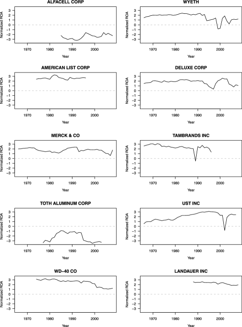
Figure 2: The performance trajectories for the ten firms with the highest posterior probabilities of having a nonzero mean.

These results are best thought of as a reasonable upper bound to the actual number of sustained superior performers. This is true for at least two reasons. First, although we used all data for 53,038 firms to fit the regression tree models and compute $m_{it}$ and $s_{it}$, we did not conduct hypothesis tests for the 16,024 firms with less than 5 years of data. It is difficult to know what “long-term superiority” even means for this vast group of firms with so short a history. Moreover, their presence in the testing stage of the analysis would likely bias the estimate of $w$ (the prior inclusion probability) downward, because the Bayes factor so strongly favors the null hypothesis for such a short trajectory. (This results from the well-known Bayesian “Occam’s razor” effect that arises when comparing models of different dimensionality.) This introduces a possible survivorship bias into our procedure. But given the assumption of exchangeability in our model, we believe that the effects of survivorship bias are less severe than the likely effects of watering down the cohort with so many firms for which the null hypothesis is so likely a priori.

Second, and more importantly, our analysis assumes that a company’s ROA result in year $t$ is independent of results from previous years, given the peer group mean and standard deviation. This is unlikely to be exactly true, and therefore introduces an upward bias in our estimate of the number of superior performers (due to the fact that autocorrelation reduces the effective sample size available for testing $H_{0}$).

One way of accounting for this bias is to introduce specific parametric assumptions about the nature of a “true null” trajectory. Indeed, this is an active and promising area of research in both this and in parallel fields (e.g., time-course microarray data). Our focus on this paper, however, is on large-scale screening with relatively few assumptions. We therefore eschew explicit parametric longitudinal models and adopt the following alternative strategy in an attempt to get a fast, crude assessment of how the independence assumption may affect our results: [(1)]

For each firm in the testing cohort, we estimate a one-lag autocorrelation coefficient, $\hat{\phi}_{i}$. For the handful of firms for which this estimate is negative, we threshold at zero, since we do not wish to introduce negative correlation into the sampling distribution for the data.

We compute an effective sample size for each trajectory as

$$\hat{n}_{i}=n_{i}\cdot\biggl{(}\frac{1-\hat{\phi}_{i}}{1+\hat{\phi}_{i}}\biggr{)}$$

using the well-known correction for autocorrelation. While this is motivated by simple AR(1)-type null models, one may interpret the multiplicative term involving $\hat{\phi}$ purely as a deflator, corresponding to the reduction in information in each longitudinal sample compared to the i.i.d. case.

We recompute the $z$-score as $\hat{z}_{i}=\bar{z}_{i}\sqrt{\hat{n}_{i}}$. We then repeat the testing procedure using the $\hat{z}_{i}$’s as data, which has the effect of inflating the variance under the null hypothesis. This correction led to 262 firms with a posterior probability greater than $90\%$ (expected FDR for the group: $2\%$), and an additional 222 with a posterior probability between $50\%$ and $90\%$ (expected FDR for the group: $26\%$). The top 10 firms remained unchanged, except for Toth Aluminum and Alfacell.

Our results appear to be qualitatively similar to those of Henderson, Raynor and Ahmed (2009), who use essentially the same data. But we will point to two important methodological differences that likely account for any major divergence in testing outcomes. First, we use model-averaged estimates from Bayesian treed regression to estimate a conditional mean and standard deviation for every company in every year. In contrast, Henderson, Raynor and Ahmed (2009) use linear quantile regression, which is a fundamentally different—and arguably less flexible—way of accounting for conditional heteroskedasticity (which appears to be the dominant effect of covariates). Second, we adjust each company’s longitudinal results individually to account for firm-level heterogeneity with respect to autocorrelation. In contrast, Henderson, Raynor and Ahmed (2009) account for longitudinal dependence by assuming that the same semi-parametric Markov model holds across the entire population of “lucky” firms.

4.3 Comparison with the popular literature on corporate success

As a small aside, it is interesting to compare these results to the conclusions of a handful of well-known books that purport to explain corporate success. We took a small, nonscientific sample of these books, in an attempt to gauge whether the results from the multiple-testing model correspond to widely held notions about successful firms. Table 4 briefly describes these books, and indicates whether the basis for selecting the study cohort was qualitative or quantitative in nature. The books were chosen in conjunction with a group of senior management consultants at Deloitte Consulting, who judged the list to be fairly representative of the popular literature.

Table 4: The popular books selected for comparison

Title	Published	Selection method	Basis
Good to Great	2001	Companies from 1965–1981 selected on the basis of shareholder return	Quantitative
Built to Last	1994	Companies founded before 1950 that met certain success criteria	Qualitative
In Search of Excellence	1982	Surveys of executives at author-selected firms	Qualitative
Competitive Strategy	1980	Author selected examples to support theory; method unclear	Qualitative
Hidden Values	2000	Author selected examples to support theory; method unclear	Qualitative
Blueprint to a Billion	2006	Time to achieve $\$1$ billion in revenue after initial public offering	Quantitative
What Really Works	2003	Correspondence with prespecified “top management practices”	Qualitative
Stall Points	2008	Patterns of stalls and recovery in revenue growth	Quantitative
Blue Ocean Strategy	2005	Author selected examples to support theory; method unclear	Qualitative

These books follow a common recipe: start with a group of companies; identify the “successful” ones; look for patterns in their behavior; and abstract those behaviors into a small set of principles that can tell others how to run their businesses better. One important difference between these books and the approach considered here is the choice of outcome variable. In some books the outcome variable is multidimensional, and therefore richer than our choice of ROA. Thus, while comparisons are instructive, they do not support the conclusion that our study is objectively right and the others wrong. Moreover, as a referee observed, the authors of these books may have different things in mind when they define success.

Yet, collectively, these studies exhibit many unacknowledged sources of bias, which our study attempts to address. None, for example, make a serious attempt to verify statistically that the selected companies have done anything special when compared with a suitable reference population. This opens up the possibility that they have been studying companies that were lucky, rather than great—the precise null hypothesis considered in this paper. There are also serious issues with selection bias—both in terms of metric selection and of company selection—and of survivorship bias (although our study is also imperfect in this regard).

Perhaps for these reasons, serious discrepancies emerged between the popular literature and the conclusions of the multiple-testing procedure considered here. Across the nine books considered, there were 209 distinct firms that were used as case studies—some positive, some negative—and that also appeared in our cohort of firms with 5 or more years of data. Of the top ten firms flagged in the previous section, only one was mentioned in any of the 9 books: Merck, a case study in Built to Last (BTL) and In Search of Excellence (ISE). Of the 209 firms collectively mentioned in these books, only 9 appear on our list of firms with ROA trajectories significantly better than those of their peer groups, once longitudinal dependence is accounted for.

5 Final remarks

We have developed a Bayesian multiple-testing procedure based upon a heavy-tailed prior for the nonzero means. These priors form an interesting, novel class of normal variance mixtures, the hypergeometric inverted-beta class. Overall, the procedure has the nice theoretical property of a redescending score function under the alternative model, and seems to perform as well as, or better than, existing gold-standard methods. Moreover, it allows relevant Bayesian and frequentist summaries to be computed with minimal computational fuss. This property arises from the simple, known form of the marginal distribution $m(y)$.

We have applied the method to a large data set on historical corporate performance, and compared the results of our analysis to some popular books that deal with the same subject. These books appear to be studying a sample where the large majority of firms have ROA performance profiles that are statistically indistinguishable from luck. Meanwhile, there on the order of hundreds of firms (out of a group of over 37,000) whose performance is at least suggestive of a sustained advantage, and yet were not considered in these high-profile case studies.

Appendix A The proposed family of priors

A.1 Connection with classical shrinkage rules

Our new class of priors has its genesis in the large body of work on classical shrinkage rules, where a multivariate normal prior $\bolds{\beta}\sim\mathrm{N}(0,\lambda^{2}I)$ is assumed, where $\bolds{\beta}=(\beta_{1},\ldots,\beta_{p})$. Many common estimators for this problem, both Bayesian and non-Bayesian, are of the form $\hat{\bolds{\beta}}(\mathbf{y})=\{1-g(Z)\}\mathbf{y}$ for $Z=\|\mathbf{y}\|^{2}$ [e.g., James and Stein (1961), Strawderman (1971), Stein (1981), Fourdrinier, Strawderman and Wells (1998)]. The central issue is how to identify “nice” functions $g(Z)$, and how to understand priors for global variance components in terms of the behavior of the estimators they yield.

The constraint to rationality—that is, the requirement that there exists a prior $p(\kappa)$ such that, for all $Z$, $g(Z)=E(\kappa\mid Z)$ under the posterior $p(\kappa\mid Z)$—rules out a wide class of potential estimators. The function $g(Z)$ cannot, for example, be a polynomial of order two or greater. Indeed, the functional form of a $g(Z)$ that respects admissibility will typically be quite complicated.

It is natural to look in the class of estimators where $g(Z)=p(Z)/q(Z)$, a ratio of power-series expansions. One can construct such a $g(Z)$ by assuming that $(\bolds{\beta}\mid\lambda^{2})\sim\mathrm{N}(0,\lambda^{2}I)$, and then defining $\hat{\bolds{\beta}}(\lambda^{2})=\mathrm{E}(\bolds{\beta}\mid\lambda^{2},\mathbf{y})$. After removing the dependence upon $\lambda^{2}$ by marginalizing, this leads to

$$\hat{\bolds{\beta}}=E_{\lambda^{2}\mid\mathbf{y}}\{\hat{\bolds{\beta}}(\lambda^{2})\}=\{1-E(\kappa\mid Z)\}\mathbf{y},$$

recalling that $\kappa=1/(1+\lambda^{2})$. We can therefore identify $g(Z)$ with $E(\kappa\mid Z)$, the posterior expectation of $\kappa$, given $Z$.

One can define a class of priors for $\kappa$ indexed by $(a,b,\tau,s)$, which we call the hypergeometric inverted-beta class, such that

$$\quad g(Z) = E(\kappa\mid Z)$$

$$= \frac{a+p/2}{a+b+p/2}\frac{\Phi_{1}(b,1;a+b+p/2+1;s+Z/2,1-1/\tau^{2})}{\Phi_{1}(b,1;a+b+p/2;s+Z/2,1-1/\tau^{2})},$$

where $a$, $b$, and $\tau$ are positive real numbers; $s$ is any real number; and $\Phi_{1}$ is the degenerate hypergeometric function of two variables [Gradshteyn and Ryzhik (1965), Equations 9.261.1–9.261.3].

This $g$ is a ratio of power series, and can be computed quite rapidly for a given tuple $(a,b,\tau,s)$ and a given $Z$. It leads to a large class of admissible estimators with a wide range of possible behavior. In particular, it includes many estimators that exhibit robustness to large values of Z; many estimators that offer significant risk reduction near $Z=0$; and many that do both. This class generalizes the form noted by Maruyama (1999), which contains the positive-part James–Stein estimator as a limiting (improper) case.

A.2 Hypergeometric inverted-beta priors

The connection with multiple testing is as follows. Recall that under the alternative model, $\beta_{i}$ is conditionally normal with variance $\lambda_{i}^{2}$. Our approach is to work with the transformed variable $\kappa_{i}=1/(1+\lambda_{i}^{2})$, and to define the following prior for $\kappa_{i}$. Suppressing subscripts for the moment,

$$p(\kappa)=C^{-1}\kappa^{a-1}(1-\kappa)^{b-1}\biggl{\{}\frac{1}{\tau^{2}}+\biggl{(}1-\frac{1}{\tau^{2}}\biggr{)}\kappa\biggr{\}}^{-1}\exp(-s\kappa),$$ (4)

where $a,b,\tau>0$ and $s\in\mathbb{R}$, and where $C_{1}$ is a constant of proportionality. We denote the hypergeometric-beta prior on the $\kappa$ scale by $\kappa\sim\operatorname{HB}(a,b,\tau,s)$.

The normalizing constant

$$C=\int_{0}^{1}\kappa^{a-1}(1-\kappa)^{b-1}\biggl{\{}\frac{1}{\tau^{2}}+\biggl{(}1-\frac{1}{\tau^{2}}\biggr{)}\kappa\biggr{\}}^{-1}\exp(-s\kappa)\,\mathrm{d}\kappa$$ (5)

can be computed using hypergeometric series. Using the theory laid out in Gordy (1998) and Polson and Scott (2011), we get

$$C=e^{-s}\operatorname{Be}(a,b)\Phi_{1}(b,1,a+b,s,1-1/\tau^{2}),$$ (6)

where $\Phi_{1}$ is the degenerate hypergeometric function of two variables [Gradshteyn and Ryzhik (1965), 9.261]. This function can be calculated accurately and rapidly by transforming it into a convergent series of ${}_{2}F_{1}$ functions [Section 9.2 of Gradshteyn and Ryzhik (1965), Gordy (1998)], making evaluation of (6) quite fast for most allowable choices of the parameters.

The implied density for $\lambda_{i}^{2}$ takes the form

$$\qquad p(\lambda^{2})=C^{-1}(\lambda^{2})^{b-1}(\lambda^{2}+1)^{-(a+b)}\exp\biggl{\{}-\frac{s}{1+\lambda^{2}}\biggr{\}}\biggl{\{}\tau^{2}+\frac{1-\tau^{2}}{1+\lambda^{2}}\biggr{\}}^{-1}.$$ (7)

This is a generalization of the inverted-beta distribution, also known as Pearson’s type VI distribution. Indeed, it reduces to an inverted beta in the special case where $s=0,\tau=1$, in which case $a\lambda^{2}/b$ will follow an $F(2b,2a)$ density.

The hypergeometric inverted-beta family contains many well-known subfamilies of priors for $\kappa$. These include the beta distribution, the generalized beta distribution [McDonald and Xu (1995)], and the Gauss hypergeometric distribution [Armero and Bayarri (1994)]. The family is itself contained in the class of compound confluent hypergeometric distributions [Gordy (1998)], which has two extra parameters that are not relevant in this context. These various related families are why we call (7) the hypergeometric inverted-beta prior. The transformed density on the $\kappa$ scale resembles a beta distribution, and we call this family the hypergeometric-beta (HB) prior.

The family in (4) has one major advantage over other similar priors: there exist easily computable expressions for the posterior mean $\mathrm{E}(\beta_{i}\mid y_{i})$ and the marginal density $m_{1}(y_{i})=\int\mathrm{N}(y_{i}\mid\beta_{i},\sigma^{2})p(\beta_{i})\,\mathrm{d}\beta_{i}$ under the hypothesis that $\beta_{i}\neq 0$. We derive these expressions in Appendix B.

A.3 Shrinkage profiles

We now turn to the specification of the four hyperparameters, and to the different “local shrinkage profiles” that are accessible through different choices of these parameters.

All normal scale-mixtures have an implied shrinkage profile $p(\kappa_{i})$, which describes the amount of shrinkage toward the origin that is expected a priori. The prior’s behavior near $\kappa_{i}=0$ controls the tail weight of the marginal prior for $\beta_{i}$, while the behavior near $\kappa_{i}=1$ controls the strength of shrinkage near zero.

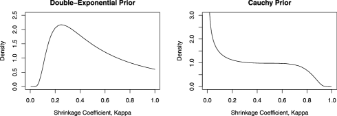
Figure 3: Implied shrinkage profiles for double-exponential and Cauchy priors.

Figure 3 plots the implied shrinkage profiles for two common priors: the double-exponential and Cauchy priors. Contrast these shrinkage profiles with the wide range of shapes that are accessible through the hypergeometric inverted-beta density, some of which are shown in Figure 4.

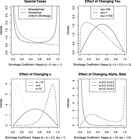
Figure 4: Effect of changing the four parameters $(a,b,s,\tau)$ on the density for the shrinkage coefficient $\kappa$.

One important special case of the hypergeometric inverted-beta family is the Strawderman prior [Strawderman (1971)], which corresponds to $a=1/2$, $b=1$, $s=0$, and $\tau=1$. Another special case is the half-Cauchy prior on the scale factor $\lambda$, studied by Gelman (2006) and Carvalho, Polson and Scott (2010). This corresponds to $a=b=1/2$, $s=0$, and $\tau=1$. Yet a third special case is the uniform-shrinkage prior, where $a=b=1$, $s=0$, and $\tau=1$. All of these can be seen in the upper-left pane of Figure 4.

Clearly, (4) can lead to many standard-looking shapes that are similar to other normal scale mixtures. Yet it can also produce a wide variety of other densities that are inaccessible through other standard families. We now describe the role of each hyperparameter, recalling that more probability near $\kappa=1$ means more aggressive shrinkage.

First, $\tau$ is a global scaling factor, with larger values leading to larger marginal variance in $\beta$. To see this, suppose that all components of $\bolds{\beta}$ have a common variance component in addition to their idiosyncratic ones: $(y_{i}\mid\beta_{i})\sim\mathrm{N}(\beta_{i},\sigma^{2})$ and $\beta_{i}\sim\mathrm{N}(0,\sigma^{2}\tau^{2}\lambda_{i}^{2})$. The form involving $\tau$ in (4) arises from the special case of assuming a half-Cauchy prior for each $\lambda_{i}$, as in the horseshoe prior of Carvalho, Polson and Scott (2010). The generalization of the scaled half-Cauchy prior to arbitrary $a$, $b$, and $s$ then arises quite naturally on the $\kappa$ scale. Shifting $\tau$ up and down causes the shrinkage profile to be shifted left and right, respectively, controlling the overall aggressiveness of shrinkage.

The parameters $a$ and $b$ are analogous to those of beta distribution, to which (4) reduces when $\tau=1$ and $s=0$. Smaller values of $a$ encourage heavier tails in $\pi(\beta$), with $a=1/2$, for example, yielding Cauchy-like tails. Smaller values of $b$ encourage $p(\beta)$ to have more mass near the origin, and eventually to become unbounded; $b=1/2$ yields, for example, $p(\beta)\approx\log(1+1/\beta^{2})$ near $0$.

Finally, $s$ is a second global scaling factor, though with a different effect than $\tau$ on the shape of the density. This parameter has an interpretation as a “prior sum of squares,” with the caveat that it can also be negative.

The scale parameters $\tau$ and $s$ do not control the behavior of $\pi(\lambda)$ at $0$ and $\infty$. Specifically, $\pi(\lambda)$ behaves like $\lambda_{i}^{2b-1}$ near the origin, and like $\lambda_{i}^{-(2a+1)}$ in the upper tail. Since $\pi(\beta)$ has the same polynomial rate of decay as $\pi(\lambda)$, $a$ can be chosen to reflect the desired tail weight of $\pi(\beta)$.

A.4 The score function and overshrinkage of exceptional observations

We recall the following theorem from Carvalho, Polson and Scott (2010).

Theorem A.1

Let $p(|y-\beta|)$ be the likelihood, and suppose that $p(\beta)$ is a mean-zero scale mixture of normals: $(\beta\mid\lambda)\sim\mathrm{N}(0,\lambda^{2})$, with $\lambda$ having proper prior $p(\lambda)$. Assume further that the likelihood and $p(\beta)$ are such that the marginal density $m(y)<\infty$ for all $y$. Define the following three pseudo-densities, which may be improper:

$$m^{\star}(y) = \int_{\mathbb{R}}p(|y-\beta|)p^{\star}(\beta)\,\mathrm{d}\beta,$$

$$p^{\star}(\beta) = \int_{\mathbb{R}^{+}}p(\beta\mid\lambda)p^{\star}(\lambda)\,\mathrm{d}\lambda,$$

$$p^{\star}(\lambda) = \lambda^{2}p(\lambda).$$

Then

$$E(\beta\mid y) = \frac{m^{\star}(y)}{m(y)}\,\frac{\mathrm{d}}{\mathrm{d}y}\log m^{\star}(y)$$

$$= \frac{1}{m(y)}\,\frac{\mathrm{d}}{\mathrm{d}y}m^{\star}(y).\vspace*{-2pt}$$

Versions of this representation theorem appear in Masreliez (1975), Polson (1991) and Pericchi and Smith (1992). Theorem A.1 relaxes a specific regularity condition having to do with the boundedness of $p(\beta)$, and extends the usual result to situations where $p(\beta)$ is a scale mixture of normals with proper mixing density and finite marginal $m(y)$.

The theorem characterizes the behavior of an estimator in the presence of large signals. Specifically, it says that we can achieve “inherent Bayesian robustness” by choosing a prior for $\beta$ such that the derivative of the log predictive density is bounded as a function of $y$. Ideally, of course, this bound should converge to $0$ for large $|y|$, and will lead to $\mathrm{E}(\theta\mid y)\approx y$ for large $|y|$. This will avoid the overshrinkage of exceptional observations—clearly an important goal in large-scale simultaneous testing problems.

It is easy to verify, using the results of the previous subsection, that normal scale mixtures with hypergeometric inverted-beta mixing distributions satisfy the property of tail robustness. This helps to explain their good performance in high-dimensional settings.

A.5 The effect of shared shrinkage parameters

The hypergeometric inverted-beta prior allows a combination of global and local shrinkage that can be both flexible and robust. Figure 5 shows how a very small value of $\tau$, encouraging strong global shrinkage, can be reinforced by a small observation ($y=1.0$), and yet be almost completely overruled by a large observation ($y=4.0$). Meanwhile, the marked bimodality for an intermediate observation such as $y=2.5$ reflects uncertainty about whether such an observation corresponds to signal or noise, with the posterior mean for $\beta$ averaging over both possibilities.

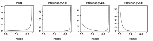
Figure 5: The left pane shows the prior for $\kappa$ when $\tau=1/15$, $s=0$, and $a=b=1/2$, reflecting a prior bias for strong shrinkage. The next three panes show the different posteriors for $\kappa$ upon observing a single data point: $y=1.0$, $y=2.5$, or $y=4.0$, respectively.

This example demonstrates that global shrinkage through $\tau$ can be very effective at squelching noise in high-dimensional problems. It is crucial, however, that $\tau$ be estimated from the data, and that the prior for $\kappa_{i}$ grow sufficiently fast near $0$ in order to allow $\kappa_{i}$ to escape the strong “gravitational pull” of a small $\tau$ when $y_{i}$ is large (as in this example when $y_{i}/\sigma=4$). We recommend setting $a=1/2$ in sparse problems involving a normal likelihood; see Carvalho, Polson and Scott (2010) for further discussion. In situations with heavier-tailed sampling models, it may be appropriate to choose a smaller value of $a$.

When $1-1/\tau^{2}$ is very close to $1$ (or when $1-\tau^{2}$ is very close to 1 for $\tau<1$), the $\Phi_{1}$ functions may become slow to evaluate due to the slow convergence of the series representations given in the Appendix. In our experience, the issue becomes practically significant in a serial computing environment only when $\tau^{2}$ is larger than 1,000 or smaller than $1/1\mbox{,}000$. Additionally, global shrinkage can take place through $s$ rather than $\tau$ (with $\tau$ being set equal to $1$). Then $\kappa_{i}\sim\operatorname{HB}(a,b,\tau=1,s)$, and so

$$(\kappa_{i}\mid y_{i})\sim\operatorname{HB}(a+1/2,b,\tau=1,s+y_{i}^{2}/2\sigma^{2}).$$

Figure 6 shows that global shrinkage through $s$ can produce results quite similar to global shrinkage through $\tau$.

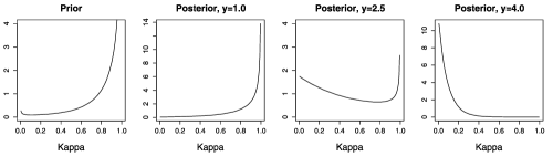
Figure 6: The left pane shows the prior for $\kappa$ when $\tau=1$, $a=b=1/2$, and $s=-4$. The next three panes show the different posteriors for $\kappa$ upon observing a single data point: $y=1.0$, $y=2.5$, or $y=4.0$, respectively.

Appendix B Expressions for moments and marginals

Throughout this section, we suppress conditioning on $\beta_{i}$’s nonzero status. Under our hypergeometric inverted-beta model, the joint distribution for $y_{i}$ and $\kappa_{i}$ takes the form

$$p(y_{i},\kappa_{i})\propto\kappa_{i}^{a^{\prime}-1}(1-\kappa_{i})^{b-1}\biggl{\{}\frac{1}{\tau^{2}}+\biggl{(}1-\frac{1}{\tau^{2}}\biggr{)}\kappa_{i}\biggr{\}}^{-1}e^{-\kappa_{i}s^{\prime}},$$

where now $s^{\prime}=s+y_{i}^{2}/(2\sigma^{2})$ and $a^{\prime}=a+1/2$.

The moment-generating function of (4) is easily shown to be

$$M(t)=e^{t}\frac{\Phi_{1}(b,1,a+b,s-t,1-1/\tau^{2})}{\Phi_{1}(b,1,a+b,s,1-1/\tau^{2})}.$$

See, for example, Gordy (1998). Expanding $\Phi_{1}$ as a sum of ${}_{1}F_{1}$ functions and using the differentiation rules given in Chapter 15 of Abramowitz and Stegun (1964) yields

$$\mathrm{E}(\kappa^{n}\mid\mathbf{y},\sigma^{2})=\frac{(a^{\prime})_{n}}{(a^{\prime}+b)_{n}}\frac{\Phi_{1}(b,1,a^{\prime}+b+n,s^{\prime},1-1/\tau^{2})}{\Phi_{1}(b,1,a^{\prime}+b,s^{\prime},1-1/\tau^{2})}.$$ (9)

Using (9), we get

$$\mathrm{E}(\beta_{i}\mid y_{i})=\biggl{\{}1-\frac{a^{\prime}}{a^{\prime}+b}\frac{\Phi_{1}(b,1,a^{\prime}+b+1,s^{\prime},1-1/\tau^{2})}{\Phi_{1}(b,1,a^{\prime}+b,s^{\prime},1-1/\tau^{2})}\biggr{\}}y.$$ (10)

And by the law of total variance,

$$\operatorname{Var}(\beta_{i}\mid y_{i}) = \mathrm{E}\{\operatorname{Var}(\beta_{i}\mid y_{i},\kappa_{i})\}+\operatorname{Var}\{\mathrm{E}(\beta_{i}\mid y_{i},\kappa_{i})\}$$

$$= \sigma^{2}\{1-\mathrm{E}(\kappa_{i}\mid y_{i})\}+y^{2}\operatorname{Var}(\kappa_{i}\mid y_{i})$$

with all other posterior moments for $\beta_{i}$ following in turn.

There is also a tractable expression for the marginal likelihood of the data:

$$m(y_{i})=C_{1}^{-1}\int_{0}^{1}\kappa_{i}^{a^{\prime}-1}(1-\kappa_{i})^{b-1}\biggl{\{}\frac{1}{\tau^{2}}+\biggl{(}1-\frac{1}{\tau^{2}}\biggr{)}\kappa_{i}\biggr{\}}^{-1}e^{-\kappa_{i}s^{\prime}}\,\mathrm{d}\kappa_{i},$$ (12)

where again $s^{\prime}=s+y_{i}^{2}/(2\sigma^{2})$ and $a^{\prime}=a+1/2$. This integral is in the same family as (5), and so by the same series of arguments we obtain

$$\qquad m(y_{i})=\frac{1}{\sqrt{2\pi\sigma^{2}}}\exp\biggl{(}-\frac{y_{i}^{2}}{2\sigma^{2}}\biggr{)}\frac{\operatorname{Be}(a^{\prime},b)}{\operatorname{Be}(a,b)}\frac{\Phi_{1}(b,1,a^{\prime}+b,s^{\prime},1-1/\tau^{2})}{\Phi_{1}(b,1,a+b,s,1-1/\tau^{2})}.$$ (13)

References

- Abramovich et al. (2006) {barticle}[mr] \bauthor\bsnmAbramovich, \bfnmFelix\binitsF., \bauthor\bsnmBenjamini, \bfnmYoav\binitsY., \bauthor\bsnmDonoho, \bfnmDavid L.\binitsD. L. and \bauthor\bsnmJohnstone, \bfnmIain M.\binitsI. M. (\byear2006). \btitleAdapting to unknown sparsity by controlling the false discovery rate. \bjournalAnn. Statist. \bvolume34 \bpages584–653. \biddoi=10.1214/009053606000000074, issn=0090-5364, mr=2281879 \bptokimsref \endbibitem
- Abramowitz and Stegun (1964) {bbook}[mr] \beditor\bsnmAbramowitz, \bfnmMilton\binitsM. and \beditor\bsnmStegun, \bfnmIrene A.\binitsI. A., eds. (\byear1964). \btitleHandbook of Mathematical Functions with Formulas, Graphs, and Mathematical Tables. \bseriesApplied Mathematics Series \bvolume55. \bpublisherNational Bureau of Standards, \baddressWashington, DC. \bnoteReprinted in paperback by Dover (1974). \bptokimsref \endbibitem
- Armero and Bayarri (1994) {barticle}[auto:STB—2011/12/07—13:41:22] \bauthor\bsnmArmero, \bfnmC.\binitsC. and \bauthor\bsnmBayarri, \bfnmM.\binitsM. (\byear1994). \btitlePrior assessments for predictions in queues. \bjournalJ. Roy. Statist. Soc. Ser. D \bvolume43 \bpages139–153. \bptokimsref \endbibitem
- Benjamini and Hochberg (1995) {barticle}[mr] \bauthor\bsnmBenjamini, \bfnmYoav\binitsY. and \bauthor\bsnmHochberg, \bfnmYosef\binitsY. (\byear1995). \btitleControlling the false discovery rate: A practical and powerful approach to multiple testing. \bjournalJ. Roy. Statist. Soc. Ser. B \bvolume57 \bpages289–300. \bidissn=0035-9246, mr=1325392 \bptokimsref \endbibitem
- Berger (1980) {barticle}[mr] \bauthor\bsnmBerger, \bfnmJames\binitsJ. (\byear1980). \btitleA robust generalized Bayes estimator and confidence region for a multivariate normal mean. \bjournalAnn. Statist. \bvolume8 \bpages716–761. \bidissn=0090-5364, mr=0572619 \bptokimsref \endbibitem
- Bogdan, Chakrabarti and Ghosh (2008) {bmisc}[auto:STB—2011/12/07—13:41:22] \bauthor\bsnmBogdan, \bfnmM.\binitsM., \bauthor\bsnmChakrabarti, \bfnmA.\binitsA. and \bauthor\bsnmGhosh, \bfnmJ. K.\binitsJ. K. (\byear2008). \bhowpublishedOptimal rules for multiple testing and sparse multiple regression. Technical Report I-18/08/P-003, Wrocław Univ. Technology. \bptokimsref \endbibitem
- Bogdan, Ghosh and Tokdar (2008) {bincollection}[mr] \bauthor\bsnmBogdan, \bfnmMałgorzata\binitsM., \bauthor\bsnmGhosh, \bfnmJayanta K.\binitsJ. K. and \bauthor\bsnmTokdar, \bfnmSurya T.\binitsS. T. (\byear2008). \btitleA comparison of the Benjamini–Hochberg procedure with some Bayesian rules for multiple testing. In \bbooktitleBeyond Parametrics in Interdisciplinary Research: Festschrift in Honor of Professor Pranab K. Sen. \bseriesInst. Math. Stat. Collect. \bvolume1 \bpages211–230. \bpublisherIMS, \baddressBeachwood, OH. \biddoi=10.1214/193940307000000158, mr=2462208 \bptokimsref \endbibitem
- Carvalho, Polson and Scott (2010) {barticle}[mr] \bauthor\bsnmCarvalho, \bfnmCarlos M.\binitsC. M., \bauthor\bsnmPolson, \bfnmNicholas G.\binitsN. G. and \bauthor\bsnmScott, \bfnmJames G.\binitsJ. G. (\byear2010). \btitleThe horseshoe estimator for sparse signals. \bjournalBiometrika \bvolume97 \bpages465–480. \biddoi=10.1093/biomet/asq017, issn=0006-3444, mr=2650751 \bptokimsref \endbibitem
- Dahl and Newton (2007) {barticle}[mr] \bauthor\bsnmDahl, \bfnmDavid B.\binitsD. B. and \bauthor\bsnmNewton, \bfnmMichael A.\binitsM. A. (\byear2007). \btitleMultiple hypothesis testing by clustering treatment effects. \bjournalJ. Amer. Statist. Assoc. \bvolume102 \bpages517–526. \biddoi=10.1198/016214507000000211, issn=0162-1459, mr=2325114 \bptokimsref \endbibitem
- Denrell (2005) {barticle}[auto:STB—2011/12/07—13:41:22] \bauthor\bsnmDenrell, \bfnmJ.\binitsJ. (\byear2005). \btitleSelection bias and the perils of benchmarking. \bjournalHarvard Business Review \bvolume83 \bpages114–119. \bptokimsref \endbibitem
- Do, Müller and Tang (2005) {barticle}[mr] \bauthor\bsnmDo, \bfnmKim-Anh\binitsK.-A., \bauthor\bsnmMüller, \bfnmPeter\binitsP. and \bauthor\bsnmTang, \bfnmFeng\binitsF. (\byear2005). \btitleA Bayesian mixture model for differential gene expression. \bjournalJ. Roy. Statist. Soc. Ser. C \bvolume54 \bpages627–644. \biddoi=10.1111/j.1467-9876.2005.05593.x, issn=0035-9254, mr=2137258 \bptokimsref \endbibitem
- Efron (2008) {barticle}[mr] \bauthor\bsnmEfron, \bfnmBradley\binitsB. (\byear2008). \btitleMicroarrays, empirical Bayes and the two-groups model. \bjournalStatist. Sci. \bvolume23 \bpages1–22. \biddoi=10.1214/07-STS236, issn=0883-4237, mr=2431866 \bptnotecheck related\bptokimsref \endbibitem
- Fourdrinier, Strawderman and Wells (1998) {barticle}[mr] \bauthor\bsnmFourdrinier, \bfnmDominique\binitsD., \bauthor\bsnmStrawderman, \bfnmWilliam E.\binitsW. E. and \bauthor\bsnmWells, \bfnmMartin T.\binitsM. T. (\byear1998). \btitleOn the construction of Bayes minimax estimators. \bjournalAnn. Statist. \bvolume26 \bpages660–671. \biddoi=10.1214/aos/1028144853, issn=0090-5364, mr=1626063 \bptokimsref \endbibitem
- Gelman (2006) {barticle}[mr] \bauthor\bsnmGelman, \bfnmAndrew\binitsA. (\byear2006). \btitlePrior distributions for variance parameters in hierarchical models (comment on article by Browne and Draper). \bjournalBayesian Anal. \bvolume1 \bpages515–533 (electronic). \bidmr=2221284 \bptnotecheck related\bptokimsref \endbibitem
- Gordy (1998) {bmisc}[auto:STB—2011/12/07—13:41:22] \bauthor\bsnmGordy, \bfnmM. B.\binitsM. B. (\byear1998). \bhowpublishedA generalization of generalized beta distributions. Finance and Economics Discussion Series 1998-18, Board of Governors of the Federal Reserve System (U.S.). \bptokimsref \endbibitem
- Gradshteyn and Ryzhik (1965) {bmisc}[auto:STB—2011/12/07—13:41:22] \bauthor\bsnmGradshteyn, \bfnmI.\binitsI. and \bauthor\bsnmRyzhik, \bfnmI.\binitsI. (\byear1965). \bhowpublishedTable of Integrals, Series, and Products. Academic Press, New York. \bptokimsref \endbibitem
- Gramacy and Lee (2008) {barticle}[mr] \bauthor\bsnmGramacy, \bfnmRobert B.\binitsR. B. and \bauthor\bsnmLee, \bfnmHerbert K. H.\binitsH. K. H. (\byear2008). \btitleBayesian treed Gaussian process models with an application to computer modeling. \bjournalJ. Amer. Statist. Assoc. \bvolume103 \bpages1119–1130. \biddoi=10.1198/016214508000000689, issn=0162-1459, mr=2528830 \bptokimsref \endbibitem
- Griffin and Brown (2005) {bmisc}[auto:STB—2011/12/07—13:41:22] \bauthor\bsnmGriffin, \bfnmJ.\binitsJ. and \bauthor\bsnmBrown, \bfnmP.\binitsP. (\byear2005). \bhowpublishedAlternative prior distributions for variable selection with very many more variables than observations. Technical report, Univ. Warwick. \bptokimsref \endbibitem
- Henderson, Raynor and Ahmed (2009) {bmisc}[auto:STB—2011/12/07—13:41:22] \bauthor\bsnmHenderson, \bfnmA. D.\binitsA. D., \bauthor\bsnmRaynor, \bfnmM. E.\binitsM. E. and \bauthor\bsnmAhmed, \bfnmM.\binitsM. (\byear2009). \bhowpublishedHow long must a firm be great to rule out luck? Benchmarking sustained superior performance without being fooled by randomness. Strategic Manag. J. To appear. DOI:10.1002/smj.1943. \bptokimsref \endbibitem
- James and Stein (1961) {bincollection}[mr] \bauthor\bsnmJames, \bfnmW.\binitsW. and \bauthor\bsnmStein, \bfnmCharles\binitsC. (\byear1961). \btitleEstimation with quadratic loss. In \bbooktitleProc. 4th Berkeley Sympos. Math. Statist. and Prob., Vol. I \bpages361–379. \bpublisherUniv. California Press, \baddressBerkeley, CA. \bidmr=0133191 \bptokimsref \endbibitem
- Jeffreys (1961) {bbook}[mr] \bauthor\bsnmJeffreys, \bfnmHarold\binitsH. (\byear1961). \btitleTheory of Probability, \bedition3rd ed. \bpublisherClarendon Press, \baddressOxford. \bidmr=0187257 \bptokimsref \endbibitem
- Johnstone and Silverman (2004) {barticle}[mr] \bauthor\bsnmJohnstone, \bfnmIain M.\binitsI. M. and \bauthor\bsnmSilverman, \bfnmBernard W.\binitsB. W. (\byear2004). \btitleNeedles and straw in haystacks: Empirical Bayes estimates of possibly sparse sequences. \bjournalAnn. Statist. \bvolume32 \bpages1594–1649. \biddoi=10.1214/009053604000000030, issn=0090-5364, mr=2089135 \bptokimsref \endbibitem
- Liang et al. (2008) {barticle}[mr] \bauthor\bsnmLiang, \bfnmFeng\binitsF., \bauthor\bsnmPaulo, \bfnmRui\binitsR., \bauthor\bsnmMolina, \bfnmGerman\binitsG., \bauthor\bsnmClyde, \bfnmMerlise A.\binitsM. A. and \bauthor\bsnmBerger, \bfnmJim O.\binitsJ. O. (\byear2008). \btitleMixtures of priors for Bayesian variable selection. \bjournalJ. Amer. Statist. Assoc. \bvolume103 \bpages410–423. \biddoi=10.1198/016214507000001337, issn=0162-1459, mr=2420243 \bptokimsref \endbibitem
- Maruyama (1999) {barticle}[mr] \bauthor\bsnmMaruyama, \bfnmYuzo\binitsY. (\byear1999). \btitleImproving on the James–Stein estimator. \bjournalStatist. Decisions \bvolume17 \bpages137–140. \bidissn=0721-2631, mr=1714127 \bptokimsref \endbibitem
- Masreliez (1975) {barticle}[auto:STB—2011/12/07—13:41:22] \bauthor\bsnmMasreliez, \bfnmC.\binitsC. (\byear1975). \btitleApproximate non-Gaussian filtering with linear state and observation relations. \bjournalIEEE Trans. Automat. Control \bvolume20 \bpages107–110. \bptokimsref \endbibitem
- McDonald and Xu (1995) {barticle}[auto:STB—2011/12/07—13:41:22] \bauthor\bsnmMcDonald, \bfnmJ. B.\binitsJ. B. and \bauthor\bsnmXu, \bfnmY. J.\binitsY. J. (\byear1995). \btitleA generalization of the beta distribution with applications. \bjournalJ. Econometrics \bvolume66 \bpages133–152. \bptokimsref \endbibitem
- McGahan and Porter (1999) {barticle}[auto:STB—2011/12/07—13:41:22] \bauthor\bsnmMcGahan, \bfnmA. M.\binitsA. M. and \bauthor\bsnmPorter, \bfnmM. E.\binitsM. E. (\byear1999). \btitleThe persistence of shocks to profitability. \bjournalRev. Econom. Statist. \bvolume81 \bpages143–153. \bptokimsref \endbibitem
- Müller, Parmigiani and Rice (2007) {bincollection}[mr] \bauthor\bsnmMüller, \bfnmPeter\binitsP., \bauthor\bsnmParmigiani, \bfnmGiovanni\binitsG. and \bauthor\bsnmRice, \bfnmKenneth\binitsK. (\byear2007). \btitleFDR and Bayesian multiple comparisons rules. In \bbooktitleBayesian Statistics 8 \bpages349–370. \bpublisherOxford Univ. Press, \baddressOxford. \bidmr=2433200 \bptnotecheck year\bptokimsref \endbibitem
- Park and Ghosh (2010) {barticle}[mr] \bauthor\bsnmPark, \bfnmJunyong\binitsJ. and \bauthor\bsnmGhosh, \bfnmJayanta K.\binitsJ. K. (\byear2010). \btitleA guided random walk through some high dimensional problems. \bjournalSankhyā \bvolume72 \bpages81–100. \biddoi=10.1007/s13171-010-0017-2, issn=0976-836X, mr=2658165 \bptokimsref \endbibitem
- Pericchi and Smith (1992) {barticle}[mr] \bauthor\bsnmPericchi, \bfnmL. R.\binitsL. R. and \bauthor\bsnmSmith, \bfnmA. F. M.\binitsA. F. M. (\byear1992). \btitleExact and approximate posterior moments for a normal location parameter. \bjournalJ. Roy. Statist. Soc. Ser. B \bvolume54 \bpages793–804. \bidissn=0035-9246, mr=1185223 \bptokimsref \endbibitem
- Polson (1991) {barticle}[mr] \bauthor\bsnmPolson, \bfnmNicholas G.\binitsN. G. (\byear1991). \btitleA representation of the posterior mean for a location model. \bjournalBiometrika \bvolume78 \bpages426–430. \biddoi=10.1093/biomet/78.2.426, issn=0006-3444, mr=1131177 \bptokimsref \endbibitem
- Polson and Scott (2011) {bmisc}[mr] \bauthor\bsnmPolson, \bfnmN. K.\binitsN. K. and \bauthor\bsnmScott, \bfnmJ. G.\binitsJ. G. (\byear2011). \bhowpublishedOn the half-Cauchy prior for a global scale parameter. Technical report, Univ. Texas at Austin. Available at arXiv:1104.4937v2. \bptokimsref \endbibitem
- Scott and Berger (2006) {barticle}[mr] \bauthor\bsnmScott, \bfnmJames G.\binitsJ. G. and \bauthor\bsnmBerger, \bfnmJames O.\binitsJ. O. (\byear2006). \btitleAn exploration of aspects of Bayesian multiple testing. \bjournalJ. Statist. Plann. Inference \bvolume136 \bpages2144–2162. \biddoi=10.1016/j.jspi.2005.08.031, issn=0378-3758, mr=2235051 \bptokimsref \endbibitem
- Stein (1981) {barticle}[mr] \bauthor\bsnmStein, \bfnmCharles M.\binitsC. M. (\byear1981). \btitleEstimation of the mean of a multivariate normal distribution. \bjournalAnn. Statist. \bvolume9 \bpages1135–1151. \bidissn=0090-5364, mr=0630098 \bptokimsref \endbibitem
- Strawderman (1971) {barticle}[mr] \bauthor\bsnmStrawderman, \bfnmWilliam E.\binitsW. E. (\byear1971). \btitleProper Bayes minimax estimators of the multivariate normal mean. \bjournalAnn. Math. Statist. \bvolume42 \bpages385–388. \bidissn=0003-4851, mr=0397939 \bptokimsref \endbibitem
- Wiggins and Ruefli (2005) {barticle}[auto:STB—2011/12/07—13:41:22] \bauthor\bsnmWiggins, \bfnmR. R.\binitsR. R. and \bauthor\bsnmRuefli, \bfnmT. W.\binitsT. W. (\byear2005). \btitleSchumpeter’s ghost: Is hypercompetition making the best of times shorter? \bjournalStrategic Management Journal \bvolume26 \bpages887–911. \bptokimsref \endbibitem
- Zellner and Siow (1980) {bincollection}[auto:STB—2011/12/07—13:41:22] \bauthor\bsnmZellner, \bfnmA.\binitsA. and \bauthor\bsnmSiow, \bfnmA.\binitsA. (\byear1980). \btitlePosterior odds ratios for selected regression hypotheses. In \bbooktitleBayesian Statistics: Proceedings of the First International Meeting Held in Valencia (\beditorJ. M. Bernardo, \beditorM. H. DeGroot, \beditorD. V. Lindley and \beditorA. F. M. Smith, eds.) \bpages585–603. \bpublisherValencia Univ. Press, \baddressValencia. \bptokimsref \endbibitem